Modelling flux tube dynamics

Abstract

Over the last few years, numerical models of the behavior of solar magnetic flux tubes have gone from using methods that were essentially one-dimensional (i.e. the thin flux tube approximation), over more or less idealized two-dimensional simulations, to becoming ever more realistic three-dimensional case studies. Along the way a lot of new knowledge has been picked up as to the e.g. the likely topology of the flux tubes, and the instabilities that they are subjected to etc. Within the context of what one could call the “flux tube solar dynamo paradigm,” I will discuss recent results of efforts to study buoyant magnetic flux tubes ascending from deep below the photosphere, before they emerge in active regions and interact with the field in the overlying atmosphere (cf. the contributions by Boris Gudiksen and Åke Nordlund): i.e. I am not addressing the flux tubes associated with magnetic bright points, which possibly are generated by a small-scale dynamo operating in the solar photosphere (cf. the contribution by Bob Stein). The presented efforts are numerical MHD simulations of twisted flux ropes and loops, interacting with rotation and convection. Ultimately the magnetic surface signatures of these simulations, when compared to observations, constraints the dynamo processes that are responsible for the generation of the flux ropes in the first place. Along with these new results several questions pop up (both old and new ones), regarding the nature of flux tubes and consequently of the solar dynamo.

1 Introduction

Buoyant magnetic flux tubes are an essential part of the framework of the current theories of dynamo action in both the Sun and solar-like stars: it is believed that when formed near the bottom of the convection zone (CZ), by a combination of rotation and turbulent convection, toroidal flux tubes buoyantly ascend in the form of tubular $\Omega$-shaped loops. Rising under the influence of rotational forces, they finally emerge after a few months as slightly asymmetric and tilted bipolar magnetic regions at the surface. Many models of buoyant magnetic flux tubes are based on the thin flux tube approximation (Spruit, 1981) that treats the tubes as strings, much thinner than e.g. the local pressure scale height, moving subjected the Coriolis and drag forces. This essentially 1-d approximation is consistent with the observations when used to study the latitudes of emergence, tilt angles, and the tilt-scatter of bipolar magnetic regions on the Sun, but only if the initial field strength of the tubes are of the order of 10 times the convection equipartition value near the bottom of the CZ (D’Silva & Choudhuri, 1993; Fan et al., 1994; Caligari et al., 1995). A major problem in dynamo theory is to understand how the field strength can become so high, corresponding to an energy density 100 times larger than that of the available kinetic energy.

However, as buoyant flux tubes rise they expand and the assumption that they are thin breaks down some 20 Mm below the solar surface. Traditionally, the latter fact is taken as the main reason for “going into higher dimensions”, i.e. for submitting to 2-d (actually 2.5-d) and 3-d models. So far, a lot of questions still remain unanswered, e.g. whether the quasi-steady state topology that the flux ropes reach in the later phase of their rise in 2-d simulations (e.g. Emonet & Moreno-Insertis 1998 and Dorch et al. 1999) is stable towards perturbations from the surroundings, and whether the results found for 3-d flux ropes moving in a 1-d average static stratification, at all are valid in the more realistic case. Hence when attempting to review the status of buoyant magnetic flux tube models, there are several questions (Q’s) that one may ask. Below are a few examples:  
Q1: In general the tubes may be twisted, but how much twist is needed and warranted?
Q2: How does the tube’s twist evolve as they ascend: do they e.g. kink due to an increasing degree of twist?
Q3: Are there other instabilities besides the magnetic Rayleigh-Taylor (R-T) and kink instabilities?
Q4: How do the tubes interact with the flows within the CZ and at the surface?
Q5: What happens to the less buoyant magnetic subsurface structure as the tubes rise (the wake)?
Q6: What happens when the ropes become thick, i.e. large comparable to the local pressure scale height?
Q7: What happens at emergence? Does the field topology change (how)?
Q8: How does the twist arise? What is the appropriate initial condition?

In the following I will try to answer some of the above Q’s by reviewing some of the main results of 2-d and 3-d models of buoyant magnetic flux tubes with emphasis on the most recent results from the turn of this millennium.

2 Reference models

For my discussion of the various aspects of flux tube models in the following, I have made a number of 2-d and 3-d simulations for reference. These are simulations for several values of the characteristic field line pitch angle $\psi_{\rm R}$.

The 2-d reference simulations lack convection and the flux tubes move in a polytropic atmosphere (dynamic), while the 3-d reference models retain full hydrodynamic convection with solar-like super-granulation and down-flows (see the Appendix at the end of this paper).

To identify the models I use a terminology where the models are referred to as e.g. 3D25 for a 3-d model where the flux tube initially is twisted corresponding to a pitch angle of $\Psi_{\rm R}=25^{\rm o}$. A 2-d model with the same pitch angle is referred to as 2D25. All the reference models have plasma-$\beta$’s at the onset of the model equal to $\beta_{0}=100$. The set-up of the reference models are discussed in more detail in the Appendix, but the initial twist of the flux tubes is given by

$${\rm B}_{z}={\rm B}_{\rm 0}e^{-(r/{\rm R})^{2}}{\rm~{}and~{}}{\rm B}_{\phi}=\alpha r/{\rm R}~{}{\rm B}_{z},$$ (1)

where ${\rm B}_{z}$ is the parallel and ${\rm B}_{\phi}$ the transversal component of the magnetic field with respect to the tube’s main axis. ${\rm B}_{\rm 0}$ is the amplitude of the field, R the radius, and $\alpha$ is the field line pitch parameter. The tubes are twisted, with a maximum pitch angle of $\psi_{\rm R}=\arctan(\alpha)$, hence “rope” is a better word to describe the state of the field lines than “tube”. In the following I set the initial radius to ${\rm R}_{0}=0.177~{}{\rm H}_{\rm P0}$, i.e. the tubes are non-thin.

The wavelength $\lambda$ of the flux rope is equal to the horizontal size of the domain $\lambda=3.2~{}{\rm H}_{\rm P0}$ at the initial position of the rope where the pressure scale height is ${\rm H}_{\rm P0}=78.3$ Mm. Then the flux rope is not undular Parker-unstable even though the stratification admits this instability for ropes longer than a critical wavelength of $\sim 12~{}{\rm H}_{\rm P0}$ (Spruit & van Ballegooijen, 1982).

Primarily the behavior of the flux tubes during the initial and rise phases are discussed. When the ropes approach the upper boundary of the CZ, they enter an “emergence phase” slightly beyond the scope of this review (but see e.g. the contributions by Gudiksen and Nordlund, ibid).

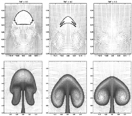
Figure 1: Flux tube disrupted by the magnetic Rayleigh-Taylor instability; from a 2-d simulation by Emonet & Moreno-Insertis (1998): The typical pitch angle was set to $7^{\rm o}$ (left), $2^{\rm o}.5$ (middle) and $0^{\rm o}$ (right). Shown are equipartition curves (top row), field strength (bottom row), and flow pattern (tiny arrows).

3 Twisted tubes

2-d simulations of flux tube cross-sections, not relying on the assumption that the flux tubes are thin, have shown that purely cylindrical tubes are quickly disrupted by the magnetic R-T instability, rendering them unlikely to reach the surface because they loose their buoyancy and cohesion (Schüssler, 1979; Tsinganos, 1980; Emonet & Moreno-Insertis, 1998; Dorch & Nordlund, 1998; Krall et al., 1998; Wissink et al., 2000).

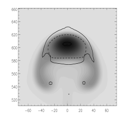
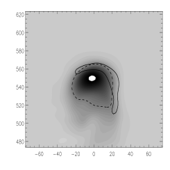
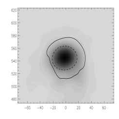
Figure 2: Images showing ${\rm B}_{z}$ at time $67.7~{}\tau_{\rm A}$ for2D30 (left), and at time $35.6~{}\tau_{\rm A}$ for 3D25 and 3D45 (center and right). Shown by contours are the equipartition curves (full curves). Also shown are HWHM-contours of ${\rm B}_{z}$ (dashed). Only a subsection of the full computational box is shown.

This apparent disruption of the tubes is a result of the too simple topology assumed for their magnetic field: rather, the magnetic field line tension present in a twisted flux rope suppresses the R-T instability and hence prevents the flux structures from disintegrating as it has been demonstrated by e.g. Emonet & Moreno-Insertis (1998): an expression similar to Eq. (1) has been applied in both 2-d and 3-d simulations and it has been shown that for these cases the R-T instability is inhibited if the degree of twist is sufficiently high as shown by Emonet & Moreno-Insertis (1998): the corresponding critical value of the field line pitch angle $\Psi_{c}$ is approximately determined by equating the energy density of the transversal (or azimuthal) field component equal to the ram pressure of the flow relative to the flux rope (incidentally, several approaches yields the same expression for $\Psi_{c}$). This kind of twist-topology is simple but similar to the relaxed state of a flux rope with a more complicated topology used in Dorch & Nordlund (1998). Emonet & Moreno-Insertis (1998) finds a critical pitch angle on the order of $arcsin(\sqrt{{\rm R}/{\rm H}_{\rm P0}})$, which typically is $10^{\rm o}$ for thin flux ropes. For thicker flux ropes, like the ones I discuss here, the value of $\Psi_{c}$ increases to approximately $25^{\rm o}$.

The boundary of a flux rope can be defined by the equipartition curve (the locations where the transversal magnetic field is in equipartition with the kinetic energy relative to the rise of the rope). Fig 1. shows equipartition curves for 2-d models by Emonet & Moreno-Insertis (1998), corresponding to three values of the pitch angle: only the most twisted ropes withstand the exterior pressure fluctuations, and the transversal field is strong enough to protect the buoyant core of the flux rope.

The results of my 2-d reference simulations agree perfectly with the 2-d studies mentioned above: the ropes are disrupted by the R-T instability unless their pitch angle exceeds a critical value. As the ropes rise and expand they enter a “terminal rise phase” where they ascent with a constant speed—while oscillating due to their differential buoyancy—before reaching the upper computational boundary (which is open). In this rise-phase the speed is the so-called terminal velocity $v_{t}$ determined by the balance between buoyancy and drag. In reference simulation 2D30—see Fig. 2 (left)—I get $v_{t}\approx 0.1~{}v_{\rm A0}$ (with $v_{\rm A0}$ being the Alfvén speed $v_{\rm A}$ at the initial position). The largest Mach number reached during the entire rise is $8.5\times 10^{-2}$, so that the motions are completely sub-sonic. The characteristic time scale of the ascent then becomes $\tau_{\rm rise}={\rm H}_{\rm P0}/v_{t}\approx 50~{}\tau_{\rm A}$ with $\tau_{\rm A}={\rm R}_{0}/v_{\rm A0}$. From the 2-d reference simulations I find that a minimum pitch angle in the range $25^{\rm o}$ – $30^{\rm o}$ is required for the ropes to be unaffected by the R-T instability, consistent with the result of Emonet & Moreno-Insertis (1998).

Consider a 3-d reference simulation with $\Psi_{\rm R}=25^{\rm o}$ (3D25): in that case the pitch is far to low to excite the kink instability (see next Section), but we expect to re-find the R-T instability in addition to the action of the convective flows. Fig 2. (center and right) shows cross-sectional averages of the magnetic field in 3D25 and 3D45 which may be compared to the corresponding image from 2D30 (note the difference in vertical offset). In the 2-d case, the horizontal and vertical sizes of the ropes do not increase equally fast. This effect is primarily because of the differential buoyancy that squeezes the ropes in the vertical direction, and by flux conservation, expands them horizontally. The effect is less apparent in 3-d, where the ropes are more circular (see Fig 2) when defined by the HWHM-boundary (i.e. the half-width at half-maximum of the parallel field component). The equipartition curve, however, loses its 2-d mirror symmetry. For a less twisted rope (e.g. 3D25 in Fig. 2), as the rope rises and the R-T instability sets in, the flux rope disrupts and eventually fills the bulk of the CZ. At late stages the magnetic field forms network patches at the surface cell boundaries, while the pumping effect (Dorch & Nordlund, 2001) transports the weakest flux down towards the bottom of the CZ.

3.1 Rotation and $\Omega$-loops

It has been suggested that the value of the critical degree of twist needed to prevent the R-T instability may be unrealistically high in the 2-d case, and a smaller twist may be sufficient in the case of sinusoidal 3-d magnetic flux loops as in the simulations: Abbett et al. (2000) used their anelastic MHD code to study the buoyant rise of twisted flux loops and found that the greater the curvature of the loop at its apex, the smaller the critical pitch angle. Moreover, Abbett et al. (2001) found that including solar-like rotation and a Coriolis force when solving the MHD equations lead to less fragmentation, even of initially un-twisted buoyant flux tubes. However, the limit on $\Psi_{c}$ is not known.

3.2 Sigmoids

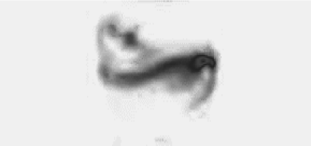
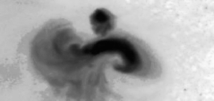
Figure 3: S-shaped structure of emerging magnetic flux rope from a simulation by Dorch et al. (1999) (left), and a sigmoid in X-ray from the Yohkoh satellite (right).

Recently, 3-d simulations of buoyant twisted flux loops have confirmed that several of the results found in the 2-d simulations carry over to the more realistic 3-d scenario (Matsumoto et al., 1998; Dorch et al., 1999; Abbett et al., 2000; Magara & Longcope, 2001). From the 3-d results it is apparent that the apex cross-sections of twisted flux loops are well described by the 2-d studies. Furthermore, the S-shaped structure of a twisted flux loop as it emerges through the upper computational boundary is qualitative similar to the sigmoidal structures observed in EUV and soft X-ray by the Yohkoh and SoHO satellites, see Fig. 3 (Canfield et al., 1999; Sterling et al., 2000).

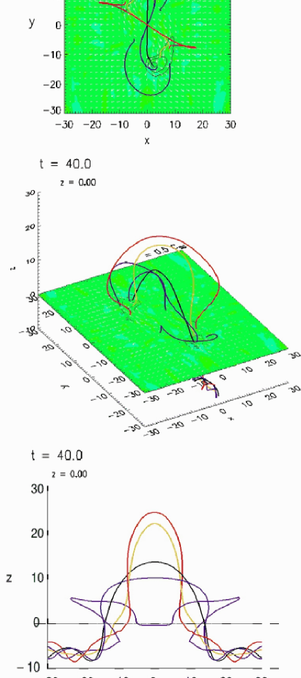
Figure 4: Snapshot of emerging twisted flux rope (dark field lines, horizontal velocity field as white arrows, vertical velocity in gray scale, and vertical magnetic field component as contours): The darkest magnetic field line is the central axis of the flux rope. Figure provided by T. Magara, e.g. Magara & Longcope (2001).

An example of such 3-d simulations are provided by Magara & Longcope (2001) who performed ideal MHD simulations of a flux rope emerging from a convection zone through a photosphere into an overlying corona: initially the flux rope is horizontal and in mechanical equilibrium, but when subjected to the undular Parker instability it is forced to rise and break through the surface, because of the buoyancy enhancing downflows along the its field lines. A similar study was performed by Fan (2001). The result is that first a magnetic bipole is formed at the surface by the oppositely directed vertical field lines of the looping flux rope. Secondly, upon emergence, a neutral line and an S-shaped (sigmoidal) structure is formed by the flux rope’s central (inner) field lines see Fig. 4. The outer field lines expand and form an S with the opposite sign of the inner one, as well as an arcadial structure with an almost potential geometry.

3.3 The flux rope’s path

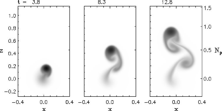
Figure 5: 2-d simulation of a buoyant flux rope rising through a stratified atmosphere; the rope follows a zigzag trajectory. Figure provided by T. Emonet, e.g. Emonet et al. (2001).

The naivistic view of a buoyant flux rope ascending nicely on a straight vertical (i.e. strictly speaking radial) path towards the surface can be dismissed qualitatively; in the 3-d case with convection, it is easy to imaging that the rope will be influenced by convective flows and be pushed around, as we shall see below. However, even in 2-d, neglecting flows that is not connected with the rope’s buoyant rise, a more subtle effect courses the ropes to have very complex trajectories when the Reynolds number becomes sufficiently large: Emonet et al. (2001) found a zig-zag motion of the magnetic flux rope caused by the imbalance of vorticity in the flux tubes, see Fig. 5. Vorticity generated when flux ascend supply a lift force; it is by this mechanism that weakly twisted flux ropes loose their updrift (negative lift force from two vortex rolls). At high viscous Reynolds number the shredding of vortex rolls in the trailing Karman-like wave of the flux introduces a vorticity-imbalance, resulting in an alternating lift force shuffling the rising rope. Perhaps surprisingly, it turns out that the complicated path of the flux rope can be described by a single non-dimensional number.

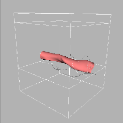
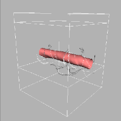
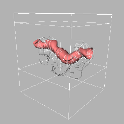
Figure 6: Snapshots of magnetic field isosurfaces at time $t=28~{}\tau_{\rm A}$ for the simulations (left to right) 3D25 (weak twist, R-T unstable), 3D45 (stable rope) and 3D75 (strong twist, kink unstable rope): the magnetic field isosurfaces outline the HWHM surfaces.

In the case 3D45, the degree of twist is small enough to prevent the onset of the kink instability (the linear ideal growth rate vanishes for $\alpha=1$, e.g. Fan et al. 1999), yet it is large enough to prevent also the onset of the R-T instability: Fig. 6 illustrates the effect of these instabilities on the shape of the flux ropes. Thus, in 3D45 the rope retains its cohesion without distorting its shape by any of these two instabilities, and we may focus our attention on the effects of the convective flows on the rope.

Figure 7: (a) Height of the flux rope as a function of time (3D45, stars and 2D45, diamonds). The straight line corresponds to the average speed of $0.1~{}v_{\rm A0}$ in the rise phase. (b) Average drift of the 3D45 flux rope in the meridional plane.

The initial position of the ropes in the CZ is significant for the subsequent detailed history of their rise: with the present flows and location of the flux ropes, most parts of the ropes are incidentally located inside or close to a convective updraft. Thus, the ascent of the ropes are influenced by this: Fig 7. compares 3D45 to 2D45 (i.e. to a convection-less reference simulation), and a simple analytic flux tube. As the 3-d rope rises, convective flows perturb its motion, preventing it from entering a rise phase with a constant rise speed, as it indeed does in 2D45 (see Fig 7a.) The rope remains straight and the maximum excursion of its axis, at the end of the simulation, is $\sim 0.04~{}\lambda$. With the chosen super-equipartition axial field strength, the main action of the large-scale convective flows is to push the rope both left and right of the central plane (Fig 7b. — see also the movie on the CD-rom), while the effect of the small-scale downdrafts is to locally deform its equipartition boundary.

The initial location within a general updraft region explains why the rise speed of the rope is slightly greater than that of the reference simulation, which reaches a terminal speed of $\sim 0.1~{}v_{\rm A0}$. The 3-d rope also expands more quickly than the rope in the 2-d simulation (see Fig. 9), but its rate of expansion is closer to what is expected from an adiabatically expanding, non-stretching tube with constant flux.

4 Kinking ropes

Fan et al. (1999) report on 3-d non-convective simulations of buoyant kink-unstable flux ropes in a stratified atmosphere, and found that a twisted flux rope becomes significantly unstable only when the pitch parameter $\alpha$ is well above a critical ideal-MHD value $\alpha_{c}=1$, i.e. if $\psi_{\rm R}>45^{\rm o}$: in the resistive-MHD case $\alpha_{c}$ increases slightly. In reference simulation 3D75 a kink therefore develops, with a maximum ideal growth rate of $\Gamma_{\rm kink}\propto\tau_{\rm A}^{-1}(\alpha^{2}-1)$ (from Linton et al. 1998), yielding a characteristic time scale of $\Gamma_{\rm kink}^{-1}\approx 0.29~{}\tau_{\rm A}$ significantly shorter than the rise time derived from the 2-d reference simulation 2D75, see Fig. 6. Diffusion decreases the growth rate further, but the instability still sets in rather quickly, well before the rope reaches the surface: the rope has plenty of time to kink while rising.

I do not invoke a perturbation of the rope’s mass or entropy to onset the kink, as do e.g. Abbett et al. (2000) and others. Rather I let the rope be perturbed by the convective flows. The power of the convection at the initial position of the rope is predominantly at long wavelengths (100 Mm), and these wavelengths of the unstable kink modes dominate the rope’s evolution.

Figure 8: Simulation vector magnetogram of an emerging kinked rope showing the horizontal (arrows) and vertical magnetic field (contours), adopted from Fan et al. (1999).

As the rope kinks, it develops a significant curvature and a knotty shape with portions dominated by vertical field components, see Fig. 6 (right). Upon emergence the bipole rotates and the neutral line between the two main polarities are strongly sheared, see Fig. 8. Hence, when the rope approaches the surface, it contains adjacent mixed polarities in horizontal cross-sections (see the CD-rom movies); this is reminiscent of the appearance of $\delta$-type sunspots with different polarities within a common umbra, and kinked flux tubes are often quoted as possibly being responsible for this phenomenon.

5 Loosing flux

Petrovay & Moreno-Insertis (1997) suggested that turbulent erosion of magnetic flux tubes may take place due to the “gnawing” on a flux tube’s field lines by turbulent convection: the flux tube is eroded by a thin current sheet forming spontaneously within a diffusion time.

Figure 9: Expansion of the flux rope (3D45, stars and 2D45, diamonds) in units of its initial radius. Also plotted is an analytical expression (solid line, see text).

Fig 9 shows the 3D45-rope’s characteristic radius ${\rm R}_{\rm hwhm}$ along its axis (with the radius defined as the average HWHM). As the rope rises and expands, its magnetic field strength also decreases to approximately conserve the flux (the decrease found in 3D45 is at a rate close but not identical to that expected for a flux-conserving tube). The deviation can be attributed to the fact that, during its ascent, magnetic flux within the 3-d rope is lost to its surroundings.

Figure 10: Left: magnetic flux within the rope $\Phi_{i}$ (3D45, stars and 2D45, diamonds) and an analytic fit (solid curve), Right: the normalized flux outside and above the center of the 3D45 rope $\Phi_{u}$ (stars), and below, $\Phi_{l}$ (triangles). The same quantities are shown for 2D45 simulation (solid and dashed curves respectively).

This is illustrated in Fig 10. (left), which shows the total normalized magnetic flux within the rope’s HWHM-core $\Phi_{i}$ as a function of time for both the 2-d and 3-d ropes (2D45 and 3D45). As the 3-d simulation progresses, the total flux-loss from the computational domain is only 0.3$\%$ — the flux content of the rope, however, decreases more rapidly.

Also shown in Fig 10. (right) is the magnetic flux external to the rope $\Phi_{e}$ both above and below its center $\Phi_{u}$ and $\Phi_{l}$ respectively. Since the sum $\Phi_{e}+\Phi_{i}$ is nearly conserved, as $\Phi_{i}$ decreases, $\Phi_{e}=\Phi_{u}+\Phi_{l}$ must increase by an equal amount. However, the distribution of the flux-loss is not symmetric around the rope: more flux is lost to the surroundings below the rope than above it.

This asymmetry also exists in 2-d, even though the total flux-loss is much smaller in that case. The asymmetry is a result of two factors. As the rope rises, the total volume above it decreases, while the volume below it increases. Furthermore, there is an anti-symmetry of the relative rise velocity across the rope: when the rope ascends, there is a tendency for flux to be advected towards it near its apex, and transported away from it in its wake. The more pronounced asymmetry in the 3-d case can be attributed to the pumping effect that transports the weak field downwards (Dorch & Nordlund, 2001).

We have defined the flux rope as the core magnetic structure that lies within the HWHM-boundary. This boundary is not, however, a contour that moves with the fluid in the classical sense: the flux within the latter kind of contour is naturally conserved (in ideal MHD) and is equal to the total flux $\Phi_{e}+\Phi_{i}$. The HWHM-boundary is a convenient way of defining the flux rope and a characteristic size ${\rm R}_{\rm hwhm}$, that behaves as it is expected to. The evolution of the flux within the rope’s core $\Phi_{i}$ is determined by the integral of $\Delta{\bf v}\times{\bf B}$ along the rope’s boundary, where $\Delta{\bf v}$ is the difference between the fluid velocity and the motion of the HWHM-boundary: the average “slip” $\Delta v$ is only a small fraction of the rise speed.

Making the rather crude assumptions that the boundary only moves radially relative to the fluid and that the circumference of the boundary is circular (which it is certainly not, but see Fig. 2), the flux-loss becomes

$$\dot{\Phi}_{i}=-\pi{\rm R}_{\rm hwhm}~{}\Delta v~{}{\rm B}_{c},$$ (2)

where ${\rm B}_{c}$ is the field strength at the center of the flux rope. Integrating the equation numerically with the quantities determined from the simulation 3D45 the result is a good fit to the actual flux-loss, see Fig 10. (left)—if $\Delta v$ is set to 3 10${}^{-4}~{}v_{\rm A0}$ throughout the time span of the simulation except for a short interval of $\sim 3~{}\tau_{A}$ around $t=30~{}\tau_{\rm A}$, where $\Delta v$ changes sign, as the rope passes from one updraft to another (Dorch et al., 2001).

Finally, I do not find flux-loss via the type of enhanced diffusion in the reference simulations as proposed by Petrovay & Moreno-Insertis (1997), and rather, the flux-loss found here is entirely due to the advection of flux away from the core of the flux rope by convective motions. The turbulent erosion mechanism requires the turbulence to be resolved down to scales much below what I have implemented here, i.e. my results does not contradict the existence of the former effect. Most of the lost flux ends up in the rope’s wake and some is mixed back into the upper layers. I speculate that both types of flux-loss may take place in the Sun, and as a result, the amount of toroidal flux stored near the bottom of the solar CZ may currently be underestimated.

6 Discussion & Summary

In this review I have tried to shed light on some of the “big” questions in the theory of buoyant magnetic flux tubes. Below I summarize some of the answers (A’s) to the questions posed in the Introduction.

A1: The critical pitch angle is about $30^{\rm o}$ (for thick ropes), in the general 3-d case including (large-scale) convective flows, but without rotational effects. The result of Abbett et al. (2000) that the inclusion of rotation lowers the critical pitch angle relative to the 2-d result, comes from non-convective simulations; i.e. to finally answer this Q we need a simulation including both rotation and realistic convection.
A2: I found no evidence that the ropes kink as they rise, at least if their initial twist is low enough: one may speculate that an initially R-T unstable rope may stabilize due to the increase of the twist (which increases only slightly in the less symmetric 3-d models).
A3: There may be other instabilities associated with the motion through the uppermost strongly stratified super-adiabatic layers, but it is not know from the models presented here.
A4: Besides the shuffling of the flux ropes by the convective flows, the primary interaction is the cause of a flux-loss due to advective erosion.
A5: The weak magnetic field and the flux lost from the rising flux tubes are transported downwards by the flux pumping-effect.

A note on A4: The numerical simulations show that the interaction of a buoyant twisted flux rope with stratified convection leads to a magnetic flux-loss from the core of the rope. During the simulation, the flux rope rises 96 Mm, and loses about 25% of its original flux content. This, ceteris paribus, leads to a small increase in the amount of toroidal flux that must be stored at the bottom of the CZ during the course of the solar cycle: Solar toroidal flux ropes rise about 200 Mm before emerging as bipolar active regions. One may thus expect them to lose even more of their initial flux, which would then be pumped back towards the bottom of the CZ. Moreover, the relative slip does not remain constant throughout the rope’s rise (Dorch et al., 2001).

Of course a lot of Q’s still remain to be answered (three from my list): the most fundamental problems remaining are those of the origin of the twist, and the question of how it arises, Q8. This is not addressed by any of the models discussed here, but in my view one likely process is the generation of twisted field lines in large-scale flux bundles located near the bottom of the convection zone, connecting across the solar equator: such flux bundles would experience a rotating motion since their lower parts are located in a region rotating slower than their uppermost parts. This rotation would transmit a twist to the parts of the flux bundle a slightly higher latitudes, thereby possibly giving rise to a twisted toroidal flux system.

Appendix: Set-up of reference models

The 2-d reference simulations lack convection and the flux tubes move in a polytropic atmosphere calculated by using the mass density $\rho(x)$ and the average gas pressure $P(x)$ in a 3-d hydrodynamic convection model via $P=P_{0}(\rho/\rho_{0})^{\gamma}$, where $P_{0}$ and $\rho_{0}$ are the average quantities at the initial position of the flux tube. In the 3-d reference models the full 3-d convection model is employed.

The initial set-up of the 3-d models are twofold, consisting of a snapshot of a solar-like CZ, and of an idealized twisted magnetic flux rope. Note that in the 2-d reference models, the CZ is polytropic through-out.

The full MHD-equations are solved on a grid of 150 vertical times $105^{2}$ horizontal grid points, using the computational method by Galsgaard and others (Galsgaard & Nordlund 1997, and Nordlund, Galsgaard & Stein 1994): Typical magnetic Reynolds numbers ${\rm Re}_{\rm m}$ in non-smooth regions of the domain are of the order of a few hundred, while several orders of magnitude higher in smooth large-scale regions.

To model solar-like convection without including all the layers up to the actual surface, I use a simple expression for an isothermal cooling layer at the upper boundary of the model, restricting the effect to a thin layer. This layer is, however, far below the real boundary of the solar CZ. Horizontally the boundaries are periodic.

The hydrodynamic part of the initial condition is a snapshot from a well developed stage of a numerical “toy model” of deep solar-like convection with a gas pressure contrast of roughly 2.5 orders of magnitude in the CZ alone. The physical size of the computational box is 250 Mm in the horizontal direction and 313 Mm in the vertical. A cellular granulation pattern is generated on the CZ’s surface with a typical length scale of about 50 Mm, about twice the canonical size of solar supergranules. The typical velocity is about 200 m/s in the narrow downdrafts at the surface and slightly less in the larger upwelling regions, close to what is found for solar supergranulation.

Initially the entropy in the interior of the tube is set equal to that in the external medium. This corresponds to buoyancy a factor of $1/\gamma$ (with $\gamma=5/3$) lower than in the case of temperature balance where the buoyancy has the classical value of $1/\beta$. The initial twist of the flux tubes is given by Eq. (1). The coordinate system is chosen so that $x$ is the vertical coordinate and $z$ the coordinate along the axis which initially is parallel to the rope. The position of the rope is described by the set $(x_{c},y_{c})$, initially equal to $(x_{0},y_{0})$, where the points $(x_{c}(z),y_{c}(z))$ along the $z$-axis are the positions in the $(x,y)$ plane, where ${\rm B}_{z}$ is maximum for a given $z$-value.

From a computational point of view one have to set $\beta_{0}$ lower than the solar values ($10^{4}$ – $10^{7}$) to reduce the computational time-scale to a reasonable value. As a compromise I set the initial field strength so that $\beta_{0}=100$ yielding $e_{\rm M}/e_{\rm K}=100$ with the present convection model.

References

- Abbett et al. (2000) Abbett, W.P., Fisher, G.H., Fan, Y., 2000, ApJ 540, 548
- Abbett et al. (2001) Abbett, W.P., Fisher, G.H., Fan, Y., 2001, ApJ 546, 1194
- Caligari et al. (1995) Caligari, P., Moreno-Insertis, F., & Schüssler, M., 1995, ApJ 441, 886
- Canfield et al. (1999) Canfield, R.C., Hudson, H.S., McKenzie, D.E., 1999, Geophys. Rev. Lett. 26(6), 627
- D’Silva & Choudhuri (1993) D’Silva, S., Choudhuri, A.R., 1993, A&A 272, 621
- Dorch et al. (1999) Dorch, S.B.F., Archontis, V., Nordlund, Å., 1999, A&A 352, L79
- Dorch et al. (2001) Dorch, S.B.F., Gudiksen, B.V., Abbett, W.P., Nordlund, Å., 2001, A&A 380, 734
- Dorch & Nordlund (1998) Dorch, S.B.F., Nordlund, Å., 1998, A&A 338, 329
- Dorch & Nordlund (2001) Dorch, S.B.F., Nordlund, Å., 2001, A&A 365, 562
- Emonet & Moreno-Insertis (1998) Emonet, T., Moreno-Insertis, F., 1998, ApJ 492, 804
- Emonet et al. (2001) Emonet, T., Moreno-Insertis, F., Rast, M.P., 2001, ApJ 549, 1212
- Fan (2001) Fan, Y., 2001, ApJ 554, L111
- Fan et al. (1994) Fan, Y., Fisher, G.H., McClymont, A.N., 1994, ApJ 436, 907
- Fan et al. (1999) Fan, Y., Zweibel, E.G., Linton, M.G., Fisher, G.H., 1999, ApJ 521, 460
- Galsgaard & Nordlund (1997) Galsgaard, K., Nordlund, Å., 1997, Journ. Geoph. Res. 102, 219
- Krall et al. (1998) Krall, J., Chen, J., Santoro, R., Spicer, D.S., Zalesak, S.T., Cargill, P.J., 1998, ApJ 500, 992
- Linton et al. (1998) Linton M.G., Dahlburg, R.B., Fisher, G.H., Longcope, D.W., 1998, ApJ 507, 404
- Magara & Longcope (2001) Magara, T., Longcope, D.W., 2001, ApJ 559, L55
- Matsumoto et al. (1998) Matsumoto, R., Tajima, T., Chou, W., Okubo, A., Shibata, K., 1998, ApJ 493, L43
- Nordlund et al. (1994) Nordlund, Å., Galsgaard, K., Stein, R.F., 1994, In R.J. Rutten, C.J. Schrijver (eds.), Solar Surface Magnetic Fields NATO ASI Series 433