Differential rotation decay in the radiative envelopes of CP stars

Stars of spectral classes A and late B are almost entirely radiative. CP stars are a slowly rotating subgroup of these stars. It is possible that they possessed long-lived accretion disks in their T Tauri phase. Magnetic coupling of disk and star leads to rotational braking at the surface of the star. Microscopic viscosities are extremely small and will not be able to reduce the rotation rate of the core of the star. We investigate the question whether magneto-rotational instability can provide turbulent angular momentum transport. We illuminate the question whether or not differential rotation is present in CP stars. Numerical MHD simulations of thick stellar shells are performed. An initial differential rotation law is subject to the influence of a magnetic field. The configuration gives indeed rise to magneto-rotational instability. The emerging flows and magnetic fields transport efficiently angular momentum outwards. Weak dependence on the magnetic Prandtl number ($\sim 10^{-2}$ in stars) is found from the simulations. Since the estimated time-scale of decay of differential rotation is $10^{7}$–$10^{8}$ yr and comparable to the life-time of A stars, we find the braking of the core to be an ongoing process in many CP stars. The evolution of the surface rotation of CP stars with age will be an observational challenge and of much value for verifying the simulations.

1 Introduction

The present work was originally motivated by the existence of stars of spectral type A of which a subgroup is peculiar to their strong magnetic fields. These peculiar A and late B stars, which are collectively called CP stars, rotate significantly slower than their non-magnetic relatives. The dipole axes of the magnetic fields of CP stars have various orientations, with a tendency to larger tilts at faster rotation (Landstreet & Mathys 2000).

Young stars suffer from considerable rotational braking in particular during their pre-main sequence evolutionary phase. Angular momentum is lost partly through stellar winds in the T Tauri phase. Additional braking probably applies to T Tauri stars having an accretion disk (classical T Tauri stars – CTTS). These stars also form a slowly rotating subgroup among the T Tauri stars (Bouvier et al. 1993) just as the slow CP stars among ordinary A and late B stars. Magnetic fields exiting the accretion disk will couple to the stellar field and exert torques as well. The braking is efficient for solar-mass T Tauri stars as found by Cameron & Campbell (1993). Recently, Stȩpień (2000) proposed the analogy between the CP star subgroup and the CTTS among T Tauri stars and explains the slow CP stars by rotational locking with the disk in their pre-main-sequence phase.

If stars are considerably slowed down at the surface, how fast rotates their interior? The microscopic viscosity of stellar plasma is extremely small. We can estimate the time-scale of viscous decrease of the rotation in case of external braking simply by estimating the time-scale due to the gas’ viscosity of roughly $\nu=10$ cm²/s. For a stellar radius of $R=10^{11}$ cm, we get a viscous time-scale of $R^{2}/\nu\approx 10^{13}$ yr which is 4–5 orders of magnitudes longer than the life-time of A stars and even a thousand times more than the age of the universe. Viscous decay of the differential rotation in any radiative shell of a star is thus not applicable. As long as there is no convection providing turbulent transport of angular momentum (whose efficiency may, however, not be very high), we should expect strong differential rotation on the way from the stellar surface to the deep interior.

A differential rotation in a radiative star will be prone to the magneto-rotational instability which requires only two things: an angular velocity decreasing with axis distance and a weak magnetic field (Balbus & Hawley 1991). The question what “weak” means will be addressed in Section 2 in the discussion of the initial magnetic field used for our simulations. The instability is known to evolve quickly on the time-scale of the rotation period. It has turned out to be an efficient generator of turbulence in accretion disks. See e.g. Kitchatinov & Rüdiger (1997) for a linear global analysis and Hawley (2000) and Arlt & Rüdiger (2001) for simulations. However, the instability is as well applicable to a stellar interior as long as the angular velocity decreases with axis distance in parts of the spherical domain. The mechanism is typically termed magneto-rotational instability or Balbus-Hawley instability. It is a consequence of the local and linear MHD equations; a lower limit to the magnetic field is only imposed by the magnetic diffusivity $\eta$ which is extremely small for stellar plasma. Field geometry is also almost irrelevant for the onset of the instability. The magneto-rotational instability must be quite ubiquitous in stellar radiative zones as soon as differential rotation emerges, likely to be caused by surface braking.

We would like to address the question of how long it takes to turn the radiative envelope of the star into a uniformly rotating shell. Is there any chance to maintain a rotation profile depending only on the axis distance? The answer on whether or not differential rotation may be expected, will have consequences for the geometry of magnetic fields or possibly for their generation in CP stars.

The questions were investigated numerically. In the second Section we will describe our setup for the simulations. The third and fourth Sections deal with the hydrodynamic and magnetohydrodynamic evolutions of a thick spherical shell. We will discuss the consequences of the computations in Section 5.

2 Simulations

The simulations apply the spectral, spherical MHD code of Hollerbach (2000). The computational domain covers a full spherical shell from the inner radius $r_{\rm i}=0.2$ to the outer radius $r_{\rm o}=1.0$. We start from the non-ideal MHD equations with the kinematic viscosity $\nu$ and the magnetic diffusivity $\eta$. The time-dependent, incompressible, non-dimensional equations are then

$$\Bigl{(}\frac{\partial}{\partial t}+\@vec{u}\cdot\nabla\Bigr{)}\@vec{u} = -\nabla p+{\rm Pm}\nabla^{2}\@vec{u}+(\nabla\times\@vec{B})\times\@vec{B}$$ (1)

$$\frac{\partial\@vec{B}}{\partial t} = \nabla^{2}\@vec{B}+\nabla\times(\@vec{u}\times\@vec{B})$$ (2)

with the usual meanings of $\@vec{u}$, $\@vec{B}$, and $p$ as the velocity, magnetic field, and pressure which is not explicitly calculated in this model, but eliminated by applying the curl-operator to Eq. (1). Lengths are normalized with the radius of the sphere, $R$, times are measured in diffusion times $R^{2}/\eta$, velocities are normalized with $\eta/R$ as well as magnetic fields with $\sqrt{\mu\rho}\eta/R$. Note that the permeability $\mu$ and the density $\rho$ are constants in our approach. This normalization leads to the magnetic Prandtl number,

$${\rm Pm}=\frac{\nu}{\eta},$$ (3)

measuring the ratio of diffusive to viscous time-scales.

Instead of the physical $\@vec{u}$ and $\@vec{B}$, we integrate the potentials $e$, $f$, $g$, and $h$ which compose the physical quantities by

$$\@vec{u} = \nabla\times(e\@vec{\hat{r}})+\nabla\times\nabla\times(f\@vec{\hat{r}}),$$ (4)

$$\@vec{B} = \nabla\times(g\@vec{\hat{r}})+\nabla\times\nabla\times(h\@vec{\hat{r}}),$$ (5)

where $\@vec{\hat{r}}$ is the unit vector in radial direction. The potentials for $\@vec{u}$ and $\@vec{B}$ are decomposed into Chebyshev polynomials for the radial dependence and into spherical harmonics for the angular dependence. The representation by potentials implies that $\nabla\cdot\@vec{u}=0$ and $\nabla\cdot\@vec{B}=0$ are always fulfilled automatically.

The initial conditions for the velocity represents a rotation profile in which the angular velocity decreases with the cylinder radius, $s=r\sin\theta$, according to

$$\Omega=\frac{{\rm Rm}}{\sqrt{1+(2s)^{2q}}},$$ (6)

where Rm is the magnetic Reynolds number which is determined by the normalized angular velocity on the axis,

$${\rm Rm}=\frac{R^{2}\Omega_{0}}{\eta}.$$ (7)

This Rm will be varied in our simulations; we always put $q=2$. A profile depending on the axis distance appears to be a reasonable choice for the internal rotation of a star being prone to magnetic coupling with an accretion disk.

According to the Rayleigh criterion of hydrodynamic stability,

$$\frac{dj^{2}}{ds}>0,$$ (8)

where $j=s^{2}\Omega$ is the angular momentum per unit mass, the above rotation profile (6) will provide us with a hydrodynamically stable configuration. For large axis distances $s\gg 1$ the profile with $q=2$ would be marginally stable, but within our shell of finite radius, the Rayleigh criterion is not violated.

The construction of the initial magnetic field is based on a vertical, homogeneous field, onto which we impose a non-axisymmetric perturbation of Fourier mode $m=1$. The total initial magnetic field can be written as

$$\@vec{B}=B_{0}[\@vec{\hat{z}}+\epsilon\sin(kz+\pi/4)\@vec{\hat{x}}],$$ (9)

where $\@vec{\hat{z}}$ is the unit vector in the direction of the rotation axis and $\@vec{\hat{x}}$ is a unit vector in the equatorial plane. The wave number of the perturbation is $k=4\pi$. We added $\pi/4$ to the second term in (9) in order to provide mixed parity to the system. Equatorial and axial symmetry are thus broken allowing the system to develop flows and fields in all modes.

The initial magnetic field contains $B_{0}=100$ and $\epsilon=1$ in most of our simulations. At ${\rm Rm}=10\,000$, this configuration implies a magnetic energy which is two orders of magnitude smaller than the kinetic energy in the initial rotation (precisely $E_{\rm mag}=0.017E_{\rm kin}$). The magnetic energy is thus much smaller than the rotational energy as required for the onset of the magneto-rotational instability. In a real stellar environment, these quantities are roughly 30 orders of magnitudes apart.

We have also reduced the perturbation amplitude to $\epsilon=0.1$ in order to estimate the sensitivity of the results to this parameter. As we will see in Section 4, the onset of the magneto-rotational instability is not affected by the smaller amplitude. The decay of differential rotation takes slightly longer with a factor of 1.6 but does not increase by an order of magnitude.

Are stars in the efficient regime of the magneto-rotational instability? For accretion disks rotating according to the Keplerian law where $\Omega\sim s^{-3/2}$, the wavelength of the most unstable mode is

$$\lambda_{\rm inst}=2\pi\sqrt{16/15}\,u_{\rm A}/\Omega$$ (10)

where $u_{\rm A}=B/\sqrt{\mu\rho}$ is the Alfvén velocity (Balbus & Hawley 1998). Let us assume that the rotation profile is partly Keplerian in a star and the rotation period be 1 day. A magnetic field of 100 kG will result – for densities between 1 and $10^{2}$ g/cm³ – in wavelengths of 10 to 100 km.

At this point, we can see that the magneto-rotational instability will set in much less promptly if $\lambda_{\rm inst}>R$, thus imposing an upper limit to the magnetic field. In principle, Eq. (10) reflects the aforementioned fact that the magnetic energy must be significantly smaller than the kinetic energy in order to be called a “weak field”. For stars, this is no problem as $\lambda_{\rm inst}$ and $B$ are proportional, and the limiting magnetic fields for which $\lambda_{\rm inst}>R$ are many orders of magnitudes larger than the fields assumed in the stellar interior.

There is no lower limit for $B$ in ideal MHD, but the non-vanishing diffusivity $\eta$ leads to a minimum magnetic field necessary for the magneto-rotational instability. Essentially, the growth rate of a perturbation with $\lambda_{\rm inst}$ must be larger than the decay rate of a structure of the same wavelength. The former is independent of $\lambda$, whereas the latter changes with $\lambda^{-2}$. Balbus & Hawley (1998) give estimates of the minimum field for the limits of ${\rm Pm}\gg 1$ and ${\rm Pm}\ll 1$. Both cases lead to $B\approx 1$ G in stellar interiors, assuming $\eta=1000$ cm²/s.

Even though magnetic fields in Ap stars are well in the suitable range for instability, we have to check the applicability of our initial $B$ for the numerical model which requires a much larger magnetic diffusion. This strong diffusion makes the instability window much narrower than it is in reality. Also the stellar $\lambda_{\rm inst}$ is invisible in the simulations due to limited resolution.

Using the angular velocity of about 6000 at $s=0.6$, the lower, diffusive limit is $B=75$, while the upper constraint from the size $R$ of the domain is $B=920$. In the computational setup with ${\rm Rm}=10\,000$ and $B_{0}=100$, we obtain a wavelength of the most unstable mode of $\lambda_{\rm inst}=0.1$ near $s=0.6$. Under real conditions, the range of suitable fields spans many orders of magnitudes, since $R$ is huge and $\eta$ is extremely small.

The values of ${\rm Pm}$, ${\rm Rm}$, the initial magnetic field strength $B_{0}$ and the amplitude of the perturbation, $\epsilon$, are the free parameters in the equations. Stellar gases possess magnetic Prandtl numbers of ${\rm Pm}\approx 0.01$. Values different from unity are typically difficult to achieve by numerical schemes. Values vastly different from unity mean that the time-scales for the diffusive processes in velocity and magnetic fields differ very much and are thus hard to cover appropriately by one simulation. We will vary Pm in our MHD simulations to evaluate the reasonableness of using Pm near unity.

The velocity and magnetic field in our computational domain are decomposed into 50 Chebyshev polynomials, 100 Legendre polynomials, and 30 Fourier modes. This resolution is sufficient to resolve the above wavelength of $\lambda_{\rm inst}=0.1$ in our numerical setup. The nonlinear terms $-(\@vec{u}\cdot\nabla)\@vec{u}+(\nabla\times\@vec{B})\times\@vec{B}$ and $\nabla\times(\@vec{u}\times\@vec{B})$ are computed on a suitable number of collocation points in real space, and the spectral decomposition of these “right sides” are fed into the implicit time-stepping scheme of the linear part of Eqs. (1) and (2). First simulations with lower resolutions of $(K,L,M)=(25,30,30)$ and $(K,L,M)=(50,50,30)$ led to the same results within 3%.

The boundary condition for the flow is stress-free at the innermost and outermost radius. Vacuum conditions are imposed to the magnetic field at the inner and outer boundaries.

Figure 1: Hydrodynamical computation of the viscous decay of differential rotation. A Reynolds number of ${\rm Rm}=50\,000$ was used here

3 Hydrodynamic evolution

Before studying the magnetohydrodynamic case, we have to assess the evolution of the rotation flow without magnetic fields. This is of particular interest since the stress-free boundary conditions are not compatible with the initial azimuthal velocity profile $u_{\phi}(r\sin\theta)$. The rotation profile will lead to meridional circulations which equalize the differential rotation on the viscous time-scale. We thus determine the purely hydrodynamic decay time before we can turn to magnetic configurations and their instabilities.

We measure a decay time with $\Omega(r,\phi)$ in the equatorial plane. The quantity is averaged over $\phi$, providing a one-dimensional function of $r$. The equatorial plane was chosen just for simplicity. Function (6) is fitted to that profile varying Rm and $q$. We determine the time when $q(t)=1$ and call it the decay time $\tau_{\rm decay}$.

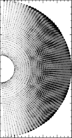
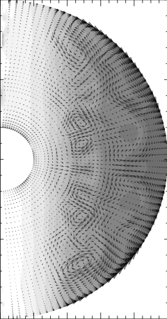
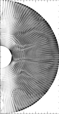
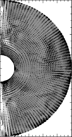
Figure 2: Series of velocity snap-shots for the model with ${\rm Rm}=10\,000$ and ${\rm Pm}=1$ at $t=0.001$, 0.002, 0.003, 0.004 diffusion times (1.6, 3.2, 4.8, and 6.4 $\tau_{\rm rot}$). The grey level contours refer to the angular velocity $u_{\phi}/s$. The scaling of these contours is the same in all four cross-sections, while the scaling of the vector lengths varies. For better visibility, we plotted only every second vector; only every third below $r=0.45$

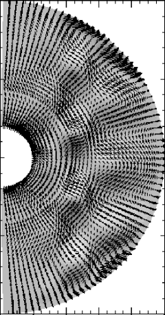
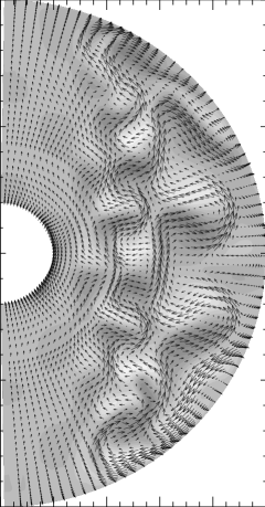
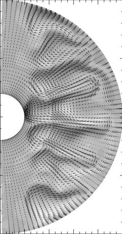
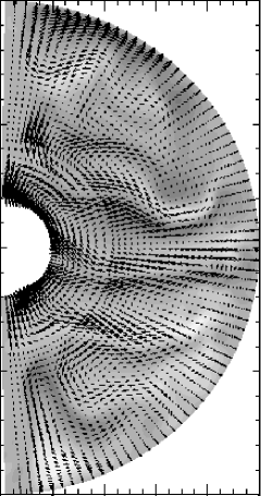
Figure 3: Series of snap-shots of the magnetic field for the model with ${\rm Rm}=10\,000$ and ${\rm Pm}=1$ at $t=0.001$, 0.002, 0.003, 0.004 diffusion times (1.6, 3.2, 4.8, and 6.4 $\tau_{\rm rot}$). The grey level contours refer to $B_{\phi}$. Again we plotted only every second vector; only every third below $r=0.45$

A model with ${\rm Rm}=10\,000$ gradually decays and reaches $q=1$ after 65 rotation periods $\tau_{\rm rot}$. We will later see that this time is much longer than the decay time caused by the magneto-rotational instability. The kinetic energy in the meridional circulation is less than 1/2000 of the energy of the azimuthal velocities. At ${\rm Rm}=50\,000$ the viscous decay lasts much longer than 200 rotation periods (Fig. 1). The ratio of azimuthal to meridional kinetic energies now exceeds $10^{4}$. Viscosities as low as stellar microscopic values are of course not achievable by numerical simulations. We can turn to magnetohydrodynamic computations knowing that the desired mechanism of differential-rotation decay should work on a time-scale of order 10 rotational periods or less to be essentially unaffected by viscosity.

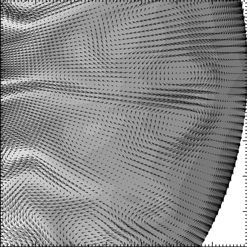
Figure 4: Detail of the velocity field shown in the third slice in Fig. 2 with full collocation point resolution

4 MHD evolution

4.1 Simulation results

The following simulations including magnetic fields regard the enhanced decay rate of differential rotation as expected from the magneto-rotational instability. An initial magnetic field as described in Eq. (9) in Section 2 causes poloidal flows with vortices of the same size as the perturbation of the magnetic field. They form in all places, except where the gradient of the angular velocity is negligible, i.e. close to the rotation axis. A series of vertical cuts through the velocity field at four equidistant times is shown in Fig. 2. The projected velocity vectors indicate that the problem is numerically resolved. Note that only every second vector of our collocation point grid is plotted for the sake of visibility; at radii smaller than 0.45 only every third vector. The same series is shown for the magnetic field in Fig. 3. The vector lengths in both graphs are not comparable among the four slices; they are scaled for best visibility.

Figure 5: Legendre spectra (latitudinal decomposition) of the energy of the magnetic field for the model with ${\rm Rm}=10\,000$ and ${\rm Pm}=1$ at three instances. Dotted line: $t=0.001$ in the beginning of the instability; solid line: $t=0.003$ during the period of strongest flows (transition period); and the dashed line: $t=0.010$ when velocity and magnetic fields decay. These times correspond to 1.6, 4.8, and $16\leavevmode\nobreak\ \tau_{\rm rot}$

The first velocity snap-shot after 1.6 orbital revolutions shows the development of cells as the direct consequence of the Lorentz forces resulting from the magnetic-field perturbation. Two counter-rotating vortices represent one wave length of the perturbation from the second term in (9). Roughly four of these waves fit into the sphere according to the wavenumber $k=4\pi$. The second slice shows the emergence of relatively thin sheets of strong radial flows in up and down directions. These features become very prominent in the third figure after $4.8\leavevmode\nobreak\ \tau_{\rm rot}$. They are actually quite extended over several tens of degrees in azimuthal direction. A detailed plot with the full resolution of our collocation point grid is shown in Fig. 4 magnifying a localized upstream. The fourth velocity slice of Fig. 2 shows an almost equalized rotation profile and a decay of small-scale features in the flow.

The latitudinal resolution of the model shown in Fig. 3 is plotted in Fig. 5 as a series of three Legendre spectra at $t=0.001$, 0.003, and 0.010, corresponding to $1.6\leavevmode\nobreak\ \tau_{\rm rot}$, $4.8\leavevmode\nobreak\ \tau_{\rm rot}$, and $16\leavevmode\nobreak\ \tau_{\rm rot}$ resp. Maximum and minimum power span 2.5 orders of magnitudes in the most turbulent case (solid line). The initial power contrast is $10^{7}$ (dotted line); after the redistribution of angular momentum, the contrast quickly reaches the same order of magnitude again (dashed line in Fig. 5). The spectra of the velocity fields are very similar. The Fourier spectra as given in Fig. 6 show very satisfying power contrast all through the simulation.

Figure 6: Azimuthal decomposition in terms of Fourier spectra of the magnetic field energy for the model with ${\rm Rm}=10\,000$ and ${\rm Pm}=1$ at the same times $t=0.001$ (dotted), 0.003 (solid), and 0.010 (dashed) as in Fig. 5

Figure 7: Redistribution of angular momentum $j$ in the model with ${\rm Rm}=10\,000$ and ${\rm Pm}=1$. The same equatorial averages as applied for the determination of the steepness $q$ were used, and $j$ was plotted for various times of the simulation in steps of $1.6\tau_{\rm rot}$; dashed lines are for $t\geq 4.8\tau_{\rm rot}$. The flat profile is from the initial rotation profile, the steep, nearly parabolic profile is the final state with almost constant angular velocity

The change of specific angular momentum as a function of axis distance is plotted in Fig. 7. The profiles of $s^{2}\Omega$ are – for simplicity – again taken from the equatorial plane and averaged over the $\phi$-direction. The initial differential rotation profile of (6) with ${\rm Rm}=10\,000$ and $q=2$ is shown as a flat curve, while the steepest, nearly parabolic lines are the final distribution of angular momentum, corresponding to a nearly uniform rotation. We plotted dashed lines for $t\geq 4.8\tau_{\rm rot}$; a gap between these and the solid lines marks the transition period when strongest transport of angular momentum is found.

The redistribution of angular momentum is a combined result of stresses from velocity and magnetic field fluctuations. The averages $\langle u_{r}^{\prime}u_{\phi}^{\prime}\rangle$ and $-\langle B_{r}^{\prime}B_{\phi}^{\prime}\rangle$, which are again taken in the equatorial plane only, show a clear domination of magnetic stresses over kinetic stresses, occasionally by a factor 10.

Figure 8: Two examples of the angular velocity averaged in the equatorial plane as a function of radius (solid lines) and the fit of (6) with ${\rm Rm}$ and $q$ (dashed lines) at $t=0.0015$ ($2.4\tau_{\rm rot}$) and $t=0.0032$ ($5.1\tau_{\rm rot}$)

In the same way as in Section 3 we measure the decay time of the differential rotation by the time it takes the system to cross a $q=1$ profile. Despite the enormous flows emerging, the azimuthally averaged angular velocity provides us with profiles $\Omega(r)$ in the equatorial plane which are fairly compatible with the two-parameter function (6). Fig. 8 shows examples of such fits for two velocity snap-shots of the simulation illustrated by snap-shots in Figs. 2 and 3. It is thus still reasonable to use the steepness $q$ for defining the decay time even for the simulations where magneto-rotational instability emerges.

The decay of $q$ with time is given by the solid line in Fig. 9. A short transition period between $4.0\leavevmode\nobreak\ \tau_{\rm rot}$ and $5.5\leavevmode\nobreak\ \tau_{\rm rot}$ can be seen. The third velocity slice of Fig. 2 with strong radial up and down flow sheets falls right in the middle of this period. Towards the end of the computation, the system oscillates around an equilibrium state with $q=0$, and magnetic and kinetic energies decay exponentially.

The transition period is less marked when we go to lower diffusivities, i.e. to higher magnetic Reynolds numbers Rm. The steepness $q$ diminishes more gradually, but still on a time-scale which is an order of magnitude shorter than viscous decay in purely hydrodynamic simulations. (Note, however, that the difference to viscous decay is expected to be much larger in a real star.) We have added the non-magnetic model with ${\rm Rm}=10\,000$ as a dashed line in Fig. 9 illustrating the marginal influence of viscous decay on the MHD simulations.

4.2 Application to stellar parameters

The rotation profile seems to decay on the rotational time-scale. This is apparently way too fast for any trace of $\Omega(s)$-rotation in stars with radiative envelopes. We will later see that this is not quite true. There are the real physical quantities which are hard to match in a computer simulation. The diffusive time-scale is orders of magnitudes longer than the rotational time-scale. We achieved to make them more than four orders of magnitudes different and may obtain an extrapolation towards real stellar parameters. The magnetic Reynolds number ${\rm Rm}={R^{2}\Omega}/{\eta}$ in stellar radiative zones is about $10^{13}$–$10^{14}$. The highest Rm achieved numerically is 50 000 in this presentation. The dependence of the decay time $\tau_{\rm decay}$ on the magnetic Reynolds number and magnetic Prandtl number is shown in Fig. 11. The decay times are given in rotation periods which is a few days for CP stars. Fortunately, we found no significant dependence of the decay times on Pm. As the true magnetic Prandtl number will be of the order of $10^{-2}$ for stars, we may assume that our Pm near unity will not imply severe differences from the real physics.

Also the amplitude $\epsilon$ of the perturbation of the initial vertical magnetic field was changed to $\epsilon=0.1$. The resulting decay of differential rotation for the model with ${\rm Rm}=10\,000$ and ${\rm Pm}=1$ is shown in Fig. 10 in terms of the steepness $q$ of the rotation profile. The decay time increased from 5 to 8 rotation periods. Also the ratio of magnetic to kinetic stresses as the constituents of the transport of angular momentum is not changed and reaches 10:1.

Figure 9: Variation of the steepness of the rotation profile with time as computed from azimuthal averages of the angular velocity of the model with ${\rm Rm}=10\,000$, ${\rm Pm}=1$, $B_{0}=100$, and $\epsilon=1$. The resulting function of $r$ was fitted to a function of the form (6). The dotted line indicates $q=1$ which will be used to define the decay time of the differential rotation. The dashed line shows the change of $q$ in a hydrodynamic model where the differential rotation decays only by viscosity

Figure 10: Variation of differential rotation of the model with ${\rm Rm}=10\,000$ as in Fig. 9. The initial perturbation of the vertical magnetic field, however, was a factor 10 smaller than there, $\epsilon=0.1$

With a series of computations with various Rm, we can make an attempt in extrapolating the decay time to stellar conditions. It is found that the decay time scales as the magnetic Reynolds number, in particular for ${\rm Rm}\geq 10\,000$ which is the interesting interval. Measured in diffusion times, the decay time depends only slightly on Rm. We derive the relation

$$\frac{\tau_{\rm decay}}{\tau_{\rm rot}}=\frac{{\rm Rm}}{2000}$$ (11)

where $\tau_{\rm rot}$ is the rotation period of the star. If the stellar parameters $R=2R_{\odot}$, $\tau_{\rm rot}=1$ day, and $\eta=1000$ cm²/s (Spitzer 1956) are applied, the magnetic Reynolds number is $3\cdot 10^{14}$. The diffusivity is the variable ingredient here; our diagram in Fig. 11 can thus be annotated with $\eta$ in stead of Rm (see upper abscissa). If Rm enters (11) with an exponent unity, the decay time is actually locked to the diffusion time and not to the rotation period. If we adopt a stellar ${\rm Pm}=10^{-2}$ and rewrite Eq. 11 as ${\tau_{\rm decay}}/{\tau_{\rm rot}}=0.0005\,{\rm Pm}\,{\rm Re}$, we see that the differential-rotation decay as a consequence of the magneto-rotational instability is of $O(10^{5})$ times faster than the viscous decay scaling with Re.

Relation (11) delivers a decay time of $3\cdot 10^{8}$ yr for the stellar parameters given above. This is of the order of the life-time of an A star. This extrapolation bears of course a wide uncertainty. If we look at the graph for ${\rm Pm}=10$ the power of Rm is slightly lower, $\tau_{\rm decay}/\tau_{\rm rot}=0.002{\rm Rm}^{0.85}$. The resulting decay time for ${\rm Rm}=3\cdot 10^{14}$ is $\tau_{\rm decay}=10^{7}$ yr.

Figure 11: Decay time of differential rotation versus magnetic Reynolds number for nine simulations with high spectral resolution. The decay time is measured in rotations. The upper abscissa gives an idea of the magnetic diffusivities $\eta$ implied by the Reynolds numbers, assuming a stellar radius and stellar rotation rate. The solid line refers to ${\rm Pm}=1$, the dashed line shows the results of ${\rm Pm}=10$. An asterisk indicates the decay time for the only computation with ${\rm Pm}=0.1$

5 Summary

Since differential rotation in radiative stellar zones cannot be damped by viscosity in a life-time of a star, we investigate the magnetic evolution which is likely to imply the onset of the magneto-rotational instability providing efficient angular-momentum transport. MHD simulations of spherical shells were performed showing that the instability emerges indeed, and quick equalization of differential rotation is found. An extrapolation to stellar parameters gives decay times of differential rotation of the order of 10–100 million years. This is the time-scale on which redistribution of angular momentum is taking place. The magneto-rotational instability grows on a scale of rotation periods, but the nett efficiency of angular momentum transport in the fully nonlinear regime is obviously a different one.

While solar-type stars have long enough life-times to rotate uniformly in their radiative cores, the life-time of stars of spectral type A is of the same order of magnitude as the decay time of about 100 million years. CP stars have magnetic fields providing the conditions for the magneto-rotational instability – along with an initial differential rotation caused by interactions with the accretion disk of the pre-main sequence life. Because of the comparable stellar life-time and decay time, differential rotation should thus be present in CP stars during a considerable period of their life. As long as the total angular momentum is conserved, we should expect a slight increase of surface angular momentum with age. Since an A star roughly doubles its radius during the presence on the main sequence, the resulting decrease of surface rotation may balance with the increase due to the mechanism described in this paper. Age data and precise rotation periods of CP stars will be needed to test this result.

References

- (1) Arlt R., Rüdiger G., 2001, A&A 374, 1035
- (2) Balbus S.A., 1995, ApJ, 453, 380
- (3) Balbus S.A., Hawley J.F., 1991, ApJ, 376, 214
- (4) Balbus S.A., Hawley J.F., 1998, Rev. Mod. Phys. 70, 1
- (5) Bouvier J., Cabrit S., Fernandez M., Martin E.L., Matthews J.M., 1993, A&A 272, 176
- (6) Cameron A.C., C.G. Campbell, 1993, A&A 274, 309
- (7) Hawley J.F., 2000, ApJ 528, 462
- (8) Hollerbach R., 2000, Int. J. Numer. Meth. Fluids, 32, 773
- (9) Kitchatinov L.L., Rüdiger G., 1997, MNRAS 286, 757
- (10) Landstreet J.D., Mathys G., 2000, A&A, 359, 213
- (11) Spitzer L.jr., 1956, Physics of fully ionized gases. Interscience Publ., New York, 81
- (12) Stȩpień K., 2000, A&A 353, 227