Understanding Scintillation of Intraday Variables

Abstract

Intraday Variability of compact extragalactic radio sources can be interpreted as quenched scintillation due to turbulent density fluctuations of the nearby ionized interstellar medium. We demonstrate that the statistical analysis of IDV time series contains both information about sub-structure of the source on the scale of several 10 $\mu$as and about the turbulent state of the ISM. The source structure and ISM properties cannot be disentangled using IDV observations alone. A comparison with the known morphology of the ‘local bubble’ and the turbulent ISM from pulsar observations constrains possible source models. We further argue that earth orbit synthesis fails for non-stationary relativistic sources and no reliable 2D-Fourier reconstruction is possible.

1 Introduction

Intraday Variability (IDV) (see Wagner & Witzel ([1995]) for a review) is a common phenomenon of flat-spectrum radio cores in quasars and BL Lacs. From light travel time arguments the observed brightness temperature of IDV sources are in the range of $10^{16\ldots 21}$ K and far in excess of the inverse Compton limit. The suggested intrinsic explanation require either extreme Doppler boosting or special source geometries. Gravitational micro-lensing and scintillation in the ISM of our galaxy are also discussed as possible propagation effects causing variability.

Two classes of IDV sources are distinguished according to their structure functions ($S\!F$). One shows a continuous increase of $S\!F$ with time-lag, while the other reaches a ‘plateau’ at a well defined time-scale $t_{\mathrm{IDV}}$ (see Fig. 1).

In this paper we will discuss the scintillation hypothesis for the ‘plateau’ class. Scintillation is caused by turbulence in the ISM, which is a stochastic process and the resulting time series are best analysed in terms of first order structure functions. Following Simonetti, Cordes & Heeschen ([1985]) we define the discrete structure function for time series $f(t_{i})$ by

$$S\!F(\tau_{j})=N^{-1}_{ij}\sum_{i=1}^{n}w(i)w(i+j)\left[f(t_{i})-f(t_{i}+\tau_{j})\right]^{2}\,.$$ (1)

Here $N_{ij}$ is the normalisation; $w(i)$ are weighting functions, so that $w(i)w(i+j)>0$, if a measurement at $t_{i}$ and another measurement at $t_{i}+\tau_{j}$ were obtained. The weighting function also accounts for bining of unevenly sampled data. The structure function is related to the autocorrelation $\rho(\tau)$ by $S\!F(\tau)=2[\rho(0)-\rho(\tau)]$.

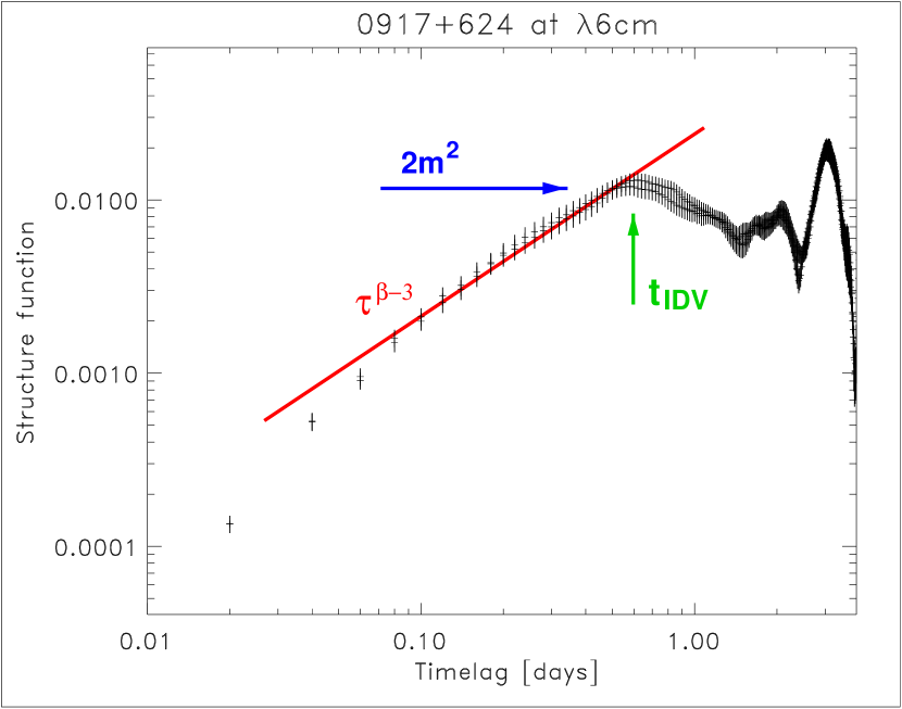
Figure 1: Structure function for IDV in total intensity for the quasar 0917+624. The $S\!F\propto\tau^{\alpha}$ has a slope of $\alpha\approx 1$, a ’plateau’ with $S\!F=2m^{2}$ for long time-lags and a characteristic timescale for decorrelation $t_{\mathrm{IDV}}$ at the first maximum.

2 Quenched Scintillation

Turbulence in the ionized ISM of our Galaxy produces density fluctuations of free electrons and the corresponding refractive index for radio wave propagation on a wide range of spatial scales (Armstrong, Rickett & Spangler [1995]). The power spectrum of density fluctuations in the ISM at wave number $q$ along the line of sight (coordinate $z$) towards the quasar is described by a power law $\Phi(z,q)=C_{N}^{2}(z)q^{-\beta}$ between a lower and upper cut-off $q_{\mathrm{low}}<q<q_{\mathrm{high}}$. The lower cut-off in $q$ corresponds to the driving wavelength of the turbulent cascade. The inertial range described by the power law ends at $q_{\mathrm{high}}$, where energy is dissipated on small spatial scales.

One distinguishes refractive and diffractive scattering at low frequencies and weak scattering above a characteristic transition frequency $\nu_{T}$ (e.g. Narayan [1992]). For quasars at high galactic latitude, the transition is expected between $1$ and $5$ GHz (e.g. Walker [1998]). The angular scale for destructive interference of wavefronts due to optical path length differences is the Fresnel scale

$$\theta_{F}=\sqrt{\frac{\lambda}{2\pi z}}=0.26\mathrm{mas}\ \left[\frac{\nu}{\mathrm{GHz}}\cdot\frac{z}{\mathrm{pc}}\right]^{-1/2}\;.$$ (2)

Large fluctuations on scales smaller than $\theta_{F}$ leads to interference and diffractive scintillation, while fluctuations on scales larger than $\theta_{F}$ act as gradients in the refractive index and causes focusing and defocusing of light rays.

Due to the ’large’ size of incoherent extragalactic synchrotron sources

$$\theta=2.1\mathrm{mas}\ \frac{(1+\tilde{z})}{\delta}\left[\frac{\nu}{\mathrm{GHz}}\right]^{-1}\left[\frac{F_{\nu}}{\mathrm{Jy}}\cdot\frac{10^{11}\ \mathrm{K}}{T_{b}}\right]^{1/2}$$ (3)

diffractive effects are unimportant, because the source size is always larger than the Fresnel scale for scattering in the ISM. Here $\tilde{z}$ is the cosmological redshift, $T_{b}$ the brightness temperature, $F_{\nu}$ the observed flux density of the source, $\nu$ the observing frequency, and $\delta$ the Doppler boosting factor.

For a scattering screen lying beyond the solar system and at frequencies $\nu\geq 1$ GHz the source size $\theta$ is always much larger than the Fresnel scale and the amplitude of variations is quenched. The amplitude of variations is reduced and the typical variability time-scale is stretched by the large size of the source.

The fluctuations in the ISM at scale $q$ change with a characteristic turbulent velocity $\tilde{v}(q)$, which is assumed much smaller than the relative velocity of earth and ISM. The scintillation pattern of intensity variations appears to be frozen in the ISM and the spatial variations are scanned by earth motion. The relative velocity of earth and ISM projected onto the sky has contributions from earth orbital motion, $v_{\mathrm{Earth}}$, the velocity of the solar system in the local standard of rest, $v_{\mathrm{LSR}}$, and the peculiar velocities of clouds and sheets in the ISM, $v_{\mathrm{cloud}}$, like those in the wall of the local bubble

$$v=v_{\mathrm{Earth}}+v_{\mathrm{LSR}}+v_{\mathrm{cloud}}\,.$$ (4)

Due to orbital motion, the velocity, $v$, traces an off-centred ellipse in the plane of the sky. The velocity transfers variations on spatial scales $x$ to temporal variations $\tau=x/v$ and leads to an annual modulation of the variability time-scale (Rickett et al. [2001]).

From theoretical considerations (Coles et al. [1987]) the autocorrelation $\rho(\tau)$ of light curves due to quenched scintillation can be calculated as an integral along the line of sight through the scattering medium of a Fourier transform $\vec{q}\rightarrow\vec{x}$

$$\rho(\vec{x})=8\pi r_{e}^{2}\lambda^{2}\int\mathrm{d}z\,\mathrm{FT}_{x\cdot q}\left\{\sin^{2}\left[\vartheta_{q}^{2}\right]\cdot\Phi(z,q)\cdot\left|V(\vec{q})\right|^{2}\right\}$$ (5)

of the geometric sinusoidal Fresnel term, the fluctuation power spectrum, and the visibility of the source surface brightness $V(q)$. The argument of the sinusoidal Fresnel term

$$\vartheta_{q}=\frac{qz}{\sqrt{2}}\theta_{F}$$ (6)

contains the Fresnel scale from (2). The Fourier transform relates the 2-D vector $\vec{x}$ in the plane of sky, given by the vector of the velocity $\vec{v}$ to the 2-D wave vector $\vec{q}$ in the scattering medium. In (5) we have neglected a refractive cut-off in Fourier space for large $q$. For quenched scintillation the first relevant cut-off in $q$ is in the visibility $V(\vec{q})$.

Anisotropic turbulence can be accounted for in $\Phi(z,\vec{q})$ but is not considered here. Non-circular and multi-component models for the source enter (5) through angular variations of the visibility in the $\vec{q}$-plane.

3 The Local ISM

The ISM of the solar neighbourhood is structured in cloudlets, sheets, and walls. The most prominent structure is the local bubble (e.g. Breitschwerdt, Freyberg & Egger [2000]) with a mean radius of $\sim 80$ pc. Perpendicular to the galactic plane this bubble extends out to about 200 pc, but its boundary is uncertain due to instabilities in the wall surrounding the bubble. The immediate vicinity of our solar system contains only small amounts of dust and a low density ionized phase out to some tens of pc. Evidence for absorption in the EUV of white dwarfs gives a mean density of 0.04 atoms/cm³, an average bubble radius of $\sim 80$ pc, and a five-fold increase in the gas density at the bubble boundary (Warwick et al. [1993]).

The amplitude of turbulence in the coronal gas of the local bubble is an order of magnitude lower than elsewhere in the ISM. This is deduced from scintillation studies of pulsars, which show reduced scintillation for the nearby pulsar 0950+08, located near the edge of the local bubble, relative to other line of sights through the ISM (Phillips & Clegg [1992]).

While quenched scintillation of extended sources favours contributions from the nearby ISM (see (10) below), the scattering material is probably associated with the wall of the local bubble. In interactions with neighbouring bubbles, radio loops are produced and the bubble interface is Rayleigh-Taylor unstable. This may have generated the large amplitude turbulence in the ionized high density gas, necessary for scintillation. For scattering in localized regions like the wall of the local bubble the scattering measure

$$S\!M=\int_{D-H/2}^{D+H/2}\mathrm{d}z\,C_{N}^{2}(z)$$ (7)

can be separated in (5) and the medium can be treated as a slab of thickness $H$ at distance $D$.

4 The Source Structure

The relation (5) between autocorrelation of intensity fluctuations and source visibility opens the path to an intensity interferometer (Hanbury Brown & Twiss [1956]). Unlike other interferometric techniques in the radio band, all phase information is lost, because scintillation in quenched scattering does not rely on constructive and destructive interference of disturbed wavefronts. The appearance of the Fresnel term and the steep power spectrum of turbulence in (5) separates the ‘IDV interferometer’ from the optical intensity interferometer and limits the angular scale to a small window in $\theta$ at which (5) can be used.

The time series of intensity fluctuations samples the autocorrelation $\rho(x)$ for different baseline lengths, $x$, in the sky but only along a given direction due to earth motion. It is therefore impossible to solve the inverse problem of (5) to get the source visibility $V(q)$ from single time series of a few days or weeks.

Even the comparison of source models and the resulting theoretical $\rho(x)$ with observed IDV is hampered by our insufficient knowledge of turbulence in the ISM. Any measurement of size and structure of the extragalactic source is affected by uncertainties in distance, scattering measure and relative velocity of the scattering medium.

From (5) we can derive the square of the modulation index $m^{2}=\lim_{\tau\rightarrow 0}\rho(\tau)$ of flux variations with a Gaussian brightness distribution for the source of width $\theta$:

$$\rho(0)=m^{2}=\left(\frac{r_{e}}{D\theta^{2}}\right)^{2}\lambda^{4}(D\theta)^{\beta-2}S\!M\cdot\frac{\Gamma(3-\beta/2)}{2}$$ (8)

But it turns out that the structure function

$$S\!F(\tau)=2\rho(0)\left(\frac{v\tau}{D\theta}\right)^{2}\frac{3-\beta/2}{4}$$ (9)

rises for small time-lags as $S\!F\propto\tau^{2}$ independent of the spectral index $\beta$. The observed $S\!F$ show always a much shallower rise (see Fig.1) with $S\!M\propto\tau^{\alpha}\,;\;\alpha=0.7\ldots 1.2$ and are inconsistent with the Gaussian model. The variability time-scale of IDV $t_{\mathrm{IDV}}$ derived from the first maximum of $S\!F$ gives the source size $\theta\approx v\,t_{\mathrm{IDV}}/(1.2\,D)$ independent of the scattering measure.

Another (extreme) source model is a disk of size $\theta$ with constant surface brightness. In this case we find

$$\rho(0)=m^{2}=2\left(\frac{r_{e}}{D\theta^{2}}\right)^{2}\lambda^{4}(D\theta)^{\beta-2}S\!M\cdot F_{1}(\beta)\ .$$ (10)

The special functions $F_{1}(\beta)$ & $G_{1}(\beta)$ are of order unity. For a succession of slabs at different distances the slab closest to the observer dominates the variations according to $m^{2}\propto S\!MD^{\beta-4}$ for power spectra $\beta<4$ and for sources larger than the Fresnel scale in the relevant slab.

The $S\!F$ for time-lags much smaller than the correlation time $t_{\mathrm{IDV}}$ rises in this case as

$$S\!F(\tau)=2\rho(0)\left(\frac{v\tau}{D\theta}\right)^{\beta-3}\frac{G_{1}(\beta)}{F_{1}(\beta)}$$ (13)

The characteristic time-scale $t_{\mathrm{IDV}}$ of IDV derived from $S\!F$ gives the source size

$$\theta=\frac{v}{D}\frac{t_{\mathrm{IDV}}}{2}$$ (14)

in this model.

The expected intrinsic brightness temperature $T_{\mathrm{b}}$ of extragalactic flat-spectrum radio cores is expected to be between the equipartition temperature of $4.7\ 10^{10}$ K and the inverse Compton limit of about $6.7\ 10^{11}$ K. For a given $T_{\mathrm{b}}$ we can estimate the distance to the scattering medium from (14) to be

$$D=137\mathrm{pc}\left[\frac{\nu}{5\mathrm{GHz}}\right]\left[\frac{T_{\mathrm{b}}}{10^{11}\mathrm{K}}\right]\left[\frac{\delta}{10}\right]\left[\frac{F_{\nu}}{1\mathrm{Jy}}\right]^{-1/2}\,.$$ (15)

where we assumed a velocity of $v=20$ km/s and $t_{\mathrm{IDV}}=1$ day. $\delta$ is the usual Doppler boosting factor and $F_{\nu}$ the observed flux density of the scintillating component. This distance agrees well with the distance to the wall of the local bubble.

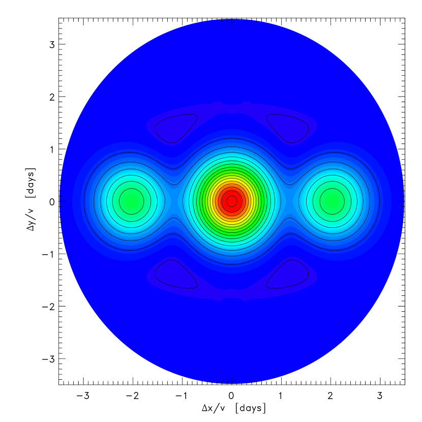
Figure 2: Autocorrelation of scintillation pattern for a two component source model. The components have Gaussian surface brightness width $\theta=50\mu$as. The separation is $7\theta$.

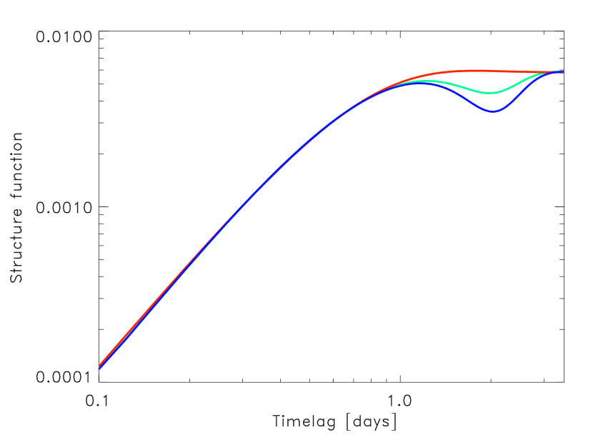
Figure 3: Structure function for a two component source model. The source model is like the one in Fig. 2. The $S\!F$ are calculated for motion along (solid), perpendicular (dashed), and at $14^{\circ}$ to the jet axis.

So far we have assumed the source to be spherically symmetric despite the fact that most IDV sources have one-sided jets.

An indication of deviation from spherical symmetry is seen in Fig. 1 where the ‘plateau’ in the structure function is not flat but has at least one minimum beyond $t_{\mathrm{IDV}}$. Besides anisotropy of turbulence in the ISM, a two-component source structure can lead to this effect as seen in Fig. 3. The autocorrelation $\rho(\vec{x})$ of a two-component model with two components of $\theta=50\mu$as each and the same flux, separated by $\theta_{2}=7\theta$ is shown in Fig. 2. $\rho(\vec{x})$ has two symmetric secondary maxima along the line connecting the two components in the sky. In such a model the minima in $S\!F$ appear only when the velocity $\vec{v}$ is within $\pm 15^{\circ}$ of the ‘jet-axis’ connecting the two components as seen from Fig. 3.

5 Earth Orbit Synthesis?

Macquart & Jauncey ([2002]) point out that the degeneracy of aligned baselines is broken by changes of earth orbit direction. Within 6 months the projected earth motion scans $180^{\circ}$ of the $\vec{v}$ ellipse in the sky. In that way the plane of $\rho(\vec{x})$ like the one in Fig. 2 can be sampled along several directions. In principle the Fourier transform of (5) can then be inverted. Besides knowledge of ISM properties as mentioned above, the source must not suffer structural changes within at least 3 months.

In the course of 3 months the distant quasar can undergo structural changes. Flat spectrum core-dominated radio sources are certainly jet-sources and emit boosted synchrotron radiation. Structural changes and flux variations of the source are limited by the light travel time for the source radius $d_{A}\theta$. For a source at a medium distance $\tilde{z}=1$ we get a lower limit on the variability time of

$$t_{\mathrm{var}}\leq 122\mathrm{days}\left[\frac{\delta}{10}\right]^{-2}\left[\frac{\nu}{5\mathrm{GHz}}\right]^{-1}\left[\frac{F_{\nu}}{1\mathrm{Jy}}\cdot\frac{10^{11}\mathrm{K}}{T_{\mathrm{b}}}\right]^{1/2}$$ (16)

which is about 4 months and therefore comparable to the required synthesis time.

6 Conclusions

Quenched scintillation gives a consistent picture of Intraday Variability for most IDV sources. The time-scale of about 1 day fits with scattering in the ionized gas of the wall of the local bubble of a moderately boosted synchrotron source with brightness temperatures below the inverse Compton limit.

From the analytic expressions for modulation index $m$ and structure function at small time-lags presented here, it is possible to determine two of the four unknowns: distance to the scattering medium, scattering measure, velocity of the medium, and size of the source. In the slab model of the scattering medium together with a constant surface brightness of the source it is possible to determine the slope $\beta\approx 4$ of turbulent power spectrum from the structure function.

The structure of IDV sources beyond the size of the most compact component cannot be uniquely determined from existing experiments. Because most IDV sources are intrinsically variable on time-scales of several months earth orbit synthesis cannot be reliably realized.

Extreme scattering events (Fiedler et al. [1987]) show that the ISM is structured on scales of several AU down to 0.01 AU (Cimò et al. [2002]) well into the scintillation domain discussed here. Turbulence in the ISM is therefore not homogeneous on scales of $v$ (3 months) = 1 AU. Changes of the long term variability pattern like the sudden end of IDV in 0917+624 (Fuhrmann et al. [2002]) can be due to changes intrinsic to the source or in the scattering measure of the ISM.

References

- [1995] Armstrong, J. W., Rickett, B. J. & Spangler, S. R. 1995, ApJ…443..209
- [2002] Beckert, T., et al. 2002, PASA, 19, 55
- [2000] Breitschwerdt, D. and Freyberg, M. J. and Egger, R. 2000, A&A, 361, 30
- [2002] Cimò, G., et al. 2002, PASA, 19, 10
- [1987] Coles, W. A., Rickett, B. J., Codona, J. L., Frehlich, R. G. 1987, ApJ, 315, 666
- [2000] Dennett-Thorpe, J. and de Bruyn, A. G. 2000, ApJ, 529, L65
- [1987] Fiedler, R. L., Dennison, B., Johnston, K. J. & Hewish, A. 1987, Natur, 326, 675
- [2002] Fuhrmann, L., et al. 2002, PASA, 19, 64
- [1956] Hanbury Brown, R., Twiss, R. Q. 1956, Nature 177, 27
- [1997] Kedziora-Chudczer, L. et al. 1997, ApJ, 490, L9
- [2002] Macquart, J.-P., Jauncey, D. L. 2002, ApJ in press, (astro-ph/0204093)
- [1992] Narayan, R. 1992, Philos. Trans. R. Soc. London, 341, 151
- [1992] Phillips J. A., Clegg Andrew W., 1992, Nature 360, 137
- [2001] Rickett, B. J., Witzel, A., Kraus, A., Krichbaum, T. P. & Qian, S. J. 2001, ApJ, 550, L11
- [1985] Simonetti, J. H. & Cordes, J. M., Heeschen, D. S. 1985, ApJ, 296, 46
- [1995] Wagner, S. J., & Witzel, A. 1995, ARA&A, 33, 163
- [1998] Walker, M. A. 1998, MNRAS, 294, 307
- [1993] Warwick R. S., Barber C. R., Hodgkin S. T., Pye J. P., 1993, MNRAS 262, 289