Parallelization Strategies for ALI Radiative Transfer in Moving Media

E. Baron Peter H. Hauschildt David Lowenthal

Abstract

We describe the method we have used to parallelize our spherically symmetric special relativistic short characteristics general radiative transfer code PHOENIX. We describe some possible parallelization strategies and show why they would be inefficient. We discuss the multiple parallelization strategy techniques that we have adopted. We briefly discuss generalizing these strategies to full 3-D (spatial) radiation transfer codes.

Dept. of Physics and Astronomy, University of Oklahoma, Norman, OK 73019-0261 USA

Dept. of Physics and Astronomy and Center for Simulational Physics, University of Georgia, Athens, GA USA

Dept. of Computer Science Physics, University of Georgia, Athens, GA USA

1. Introduction

In general parallelization is a subject to be avoided (as nicely described by P. Höflich, this volume), however in order to take advantage of the enormous computing power and vast memory sizes of modern parallel supercomputers, allowing both much faster model calculations as well as more detailed models, we have implemented a parallel version of the general model atmosphere code PHOENIX (Hauschildt & Baron 1999 and references therein). Since the code uses a modular design, we have implemented different parallelization strategies for different modules in order to maximize the total parallel speed-up of the code. Our implementation allows us to change the load distribution onto different processor elements (PEs) both via input files and dynamically during a model run, which gives a high degree of flexibility to optimize the performance on a number of different machines and for a number of different model parameters.

Since we have both large CPU and memory requirements we have implemented the parallel version of the code on using the MPI message passing library (MPI Forum 1995).

We have chosen to work with the MPI message passing interface, since it is both portable (public domain implementations of MPI are readily available cf. Gropp et al. 1996), running on dedicated parallel machines and heterogeneous workstation clusters and it is available for both distributed and shared memory architectures. For our application, the distributed memory model is in fact easier to code than a shared memory model, since then we do not have to worry about locks and synchronization, etc. on small scales and we, in addition, retain full control over interprocess communication. This is especially clear once one realizes that it is fine to execute the same code on many PEs as long as it is not too CPU intensive, and avoids costly communication. We have added a few simple OpenMP directives to our code, but do not discuss SMP parallelization further here.

An alternative to an implementation with MPI is an implementation using High Performance Fortran (HPF) directives (in fact, both can co-exist to improve performance). However, the process of automatic parallelization guided by the HPF directives is presently not yet generating optimal results because the compiler technology is still very new. HPF is also more suited for problems that are purely data-parallel (SIMD problems) and would not benefit much from a MIMD approach. An optimal HPF implementation of PHOENIX would also require a significant number of code changes in order to explicitly instruct the compiler not to generate too many communication requests, which would slow down the code significantly. The MPI implementation requires only the addition of a few explicit communication requests, which can be done with a small number of library calls.

2. Basic numerical methods

The co-moving frame radiative transfer equation for spherically symmetric flows can be found in e.g., Mihalas & Mihalas (1984). The equation of radiative transfer is a integro-differential equation, since the differential operator on the left hand side acts on the specific intensity $I_{\nu}$ , but the right hand side contains the emissivity $\eta_{\nu}$ which in turn contains $J_{\nu}$ , the zeroth angular moment of $I_{\nu}$ :

\eta_{\nu}=\kappa_{\nu}S_{\nu}+\sigma_{\nu}J_{\nu},

and

J_{\nu}=1/2\int_{-1}^{1}d\mu\,I_{\nu},

where $S_{\nu}$ is the source function, $\kappa_{\nu}$ is the absorption opacity, and $\sigma_{\nu}$ is the scattering opacity. With the assumption of time-independence $\frac{\partial I_{\nu}}{\partial t}=0$ and a monotonic velocity field the transfer equation becomes a boundary-value problem in the spatial coordinate and an initial value problem in the frequency or wavelength coordinate. The equation can be written in operator form as:

\displaystyle J_{\nu}=\Lambda_{\nu}S_{\nu},

(1)

where $\Lambda$ is the lambda-operator.

3. Parallel radiative transfer

3.1. Strategy and implementation

We use a modified version of the method discussed in Hauschildt (1992) for the numerical solution of the special relativistic radiative transfer equation (RTE) at every wavelength point (see also Hauschildt, Störzer, & Baron 1994 and Hauschildt & Baron 1999). This iterative scheme is based on the operator splitting approach. The RTE is written in its characteristic form and the formal solution along the characteristics is done using a piecewise parabolic integration (PPM, this is the “short characteristic method” Olson & Kunasz 1987). We use the exact band-matrix subset of the discretized $\Lambda$ -operator as the ‘approximate $\Lambda$ -operator’ (ALO) in the operator splitting iteration scheme (see Hauschildt et al. 1994). This gives very good convergence and high speed-up when compared to diagonal ALO’s.

The serial radiative transfer code has been optimized for superscalar and vector computers and is numerically very efficient. It is therefore crucial to optimize the ratio of communication to computation in the parallel implementation of the radiative transfer method. In terms of CPU time, the most costly parts of the radiative transfer calculation are the setup of the PPM interpolation coefficients and the formal solutions (which have to be performed in every iteration). The construction of a tri-diagonal ALO requires about the same CPU time as a single formal solution of the RTE and is thus not a very important contributor to the total CPU time required to solve the RTE at every given wavelength point.

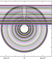
In principle, the computation of the PPM coefficients does not require any communication and thus could be distributed arbitrarily between the PEs. However, the formal solution is recursive along each characteristic. Within the formal solution, communication is only required during the computation of the mean intensities, $J$ , as they involve integrals over the angle $\mu$ at every radial point. Thus, a straightforward and efficient way to parallelize the radiative transfer calculation is to distribute sets of characteristics onto different PEs. As Auer (this volume) has emphasized, the solution of the radiative transfer equation is independent along a ray and in the sense that we treat each characteristic separately for the solution to the RTE, this parallelization step is one of domain decomposition. Figure 1 illustrates the characteristics for a typical supernova model calculation.

Refer to caption — Figure 1.: Schematic representation of the characteristic rays in a typical supernova model calculation. The curvature of the rays has been neglected in the figure, but is always included in the model calculations.

Within one iteration step, the current values of the mean intensities need to be broadcast to all radiative transfer PEs and the new contributions of every radiative transfer PE to the mean intensities at every radius must be sent to the master PE. The master radiative transfer PE then computes and broadcasts an updated $J$ vector using the operator splitting scheme, the next iteration begins, and the process continues until the solution is converged to the required accuracy. The setup, i.e., the computation of the PPM interpolation coefficients and the construction of the ALO, can be parallelized using the same method and PE distribution. The communication overhead for the setup is roughly equal to the communication required for a single iteration.

An important point to consider is the load balancing between the N_RT radiative transfer PEs. The workload to compute the formal solution along each characteristic is proportional to the number of intersection points of the characteristic with the concentric spherical shells of the radial grid (the ‘number of points’ along each characteristic). Therefore, if the total number of points is $N_{\rm P}$ , the optimum solution would be to let each radiative transfer PE work on $N_{\rm P}/N_{\rm RT}$ points. In general, this optimum cannot be reached exactly because it would require splitting characteristics between PEs (which involves both communication and synchronization). We therefore compromise by distributing the characteristics to the radiative transfer PEs so that the total number of points that are calculated by each PE is roughly the same and that every PE works on a different set of characteristics.

4. Parallelization of the line opacity calculation

The contribution of spectral lines by both atoms and molecules is calculated in PHOENIX by direct summation of all contributing lines. Each line profile is computed individually at every radial point for each line within a search window (typically, a few hundred to few thousand Doppler widths or about $1000$ Å). This method is more accurate than methods that rely on pre-computed line opacity tables (the “opacity sampling method”) or methods based on distribution functions (the “opacity distribution function (ODF) method”).

In typical model calculations we find that about 1,000 to 10,000 spectral lines contribute to the line opacity (e.g., in M dwarf model calculations) at any wavelength point, requiring a large number of individual Voigt profiles at every wavelength point. The subroutines for these computations can easily be vectorized and we use a block algorithm with caches and direct access scratch files for the line data to minimize storage requirements. A block is the number of lines stored in active memory, and the cache is the total number of blocks stored in memory. When the memory size is exceeded, the blocks are written to direct access files on disk. Thus the number of lines that can be included is not limited by RAM, but rather by disk space and the cost of I/O. This approach is computationally efficient because it provides high data and code locality and thus minimizes cache/TLB misses and page faults.

There are several obvious ways to parallelize the line opacity calculations. The first method is to let each PE compute the opacity at $N_{\rm r}/N_{\rm PE}$ radial points, the second is to let each PE work on a different subset of spectral lines within each search window. A third way, related to the second method, is to use completely different sets of lines for each PE (i.e., use a global workload split between the PEs in contrast to a local split in the second method). We discuss the advantages and disadvantages of these three methods. All three methods require only a very small amount of communication, namely a gather of all results to the master PE with an MPI_REDUCE library call.

The first and second methods, distributing sets of radial points or sets of lines within the local (wavelength dependent) search window over the PEs, respectively, are very simple to implement. They can easily be combined to optimize their performance: if for any wavelength point the number of depth points is larger than the number of lines within the local search window, then it is more effective to run this wavelength point parallel with respect to the radial points, otherwise it is better to parallelize with respect to the lines within the local window. It is trivial to add logic to decide the optimum method for every wavelength point individually. This optimizes overall performance with negligible overhead. The speed-up for this method of parallelization is very close to the optimum value if the total number of blocks of the blocking algorithm is relatively small ( $\leq 3\ldots 5$ ).

However, if the total number of line blocks is larger (typically, about 10 to 20 blocks are used), the overhead due to the read operations for the block scratch files becomes noticeable and can reach 20% or more of the total wall-clock time. This is due to the fact that the ‘local parallelization’ required that each PE working on the line opacities needs to read every line block, thus increasing the I/O time and load to the I/O subsystem by the number of PEs themselves. We discuss I/O parallelization in § 8.

5. Parallelizing NLTE calculations

Our method for iteratively solving the NLTE radiative transfer and rate equations with an operator splitting method are discussed in detail in Hauschildt (1993), and in Hauschildt & Baron (1995, 1999), therefore, we summarize our approach here only a briefly. The method uses a “rate-operator” formalism that extends the approach of Rybicki & Hummer (1991) to the general case of multi-level NLTE calculations with overlapping lines and continua, i.e, “pre-conditioning”. We use an “approximate rate-operator” that is constructed using the exact elements of the discretized $\Lambda$ -matrix (these are constructed in the radiative transfer calculation for every wavelength point). This approximate rate-operator can be either diagonal or tri-diagonal. The method gives good convergence for a wide range of applications and is very stable. It has the additional advantage that it can handle very large model atoms, e.g., we use up to 11000 levels for NLTE model atoms in regular model calculations (Hauschildt et al. 1996, Baron et al. 1996, Short et al. 1999).

Parallelizing the NLTE calculations involves parallelizing three different sections: the NLTE opacities; the rates; and the solution of the rate equations. In the following discussion, we consider only a diagonal approximate rate-operator for simplicity. In this case, the computation of the rates and the solution of the rate equations as well as the NLTE opacity calculations can simply be distributed onto a set of PEs without any communication (besides the gathering of the data at the end of the iteration). This provides a very simple way of achieving parallelism and minimizes the total communication overhead. The generalization to a tridiagonal approximate rate-operator is in principle straightforward, and involves only communication at the boundaries between two adjacent PEs.

It would be possible to use the other two methods that we discussed in the section on the LTE line opacities, namely local and global set of lines distributed to different PEs. However, both would involve an enormous amount of communication between the NLTE PEs because each NLTE transition can be coupled to any other NLTE transition. These couplings require that a PE working on any NLTE transition have the required data to incorporate the coupling correctly. Although this only applies to the PEs that work on the NLTE rates, it would require both communication of each NLTE opacity task with each other (to prepare the necessary data) and communication from the NLTE opacity PEs to the NLTE rate PEs. This could mean that several MB data would have to be transferred between PEs at each wavelength point, which is prohibitive with current communication devices.

We have implemented the parallelization of the NLTE calculations by distributing the set of radial points on different PEs. In order to minimize communication, we also ‘pair’ NLTE PEs so that each PE works on NLTE opacities, rates, and rate equations for a given set of radial points. This means that the communication at every wavelength point involves only gathering the NLTE opacity data to the radiative transfer PEs and the broadcast of the result of the radiative transfer calculations (i.e., the ALO and the $J$ ’s) to the PEs computing the NLTE rates. The overhead for these operations is negligible but it involves synchronization (the rates can only be computed after the results of the radiative transfer are known, similarly, the radiative transfer PEs have to wait until the NLTE opacities have been computed). Therefore, a good balance between the radiative transfer tasks and the NLTE tasks is important to minimize waiting. The rate equation calculations parallelize trivially over the layers and involve no communication if the diagonal approximate rate-operator is used. After the new solution has been computed, the data must be gathered and broadcast to all PEs, the time for this operation is negligible because it is required only once per model iteration.

An important problem arises from the fact that the time spent in the NLTE routines is not dominated by the floating point operations (both the number and placement of floating point operation were optimized in the serial version of the code) but by memory access, in particular for the NLTE rate construction. Although the parallel version accesses a much smaller number of storage cells (which naturally reduces the wall-clock time), effects like cache and TLB misses and page faults contribute significantly to the total wall-clock time. All of these can be reduced by using Fortran-90 specific constructs in the following way: We have replaced the static allocation of the arrays that store the profiles, rates etc. used in the NLTE calculations (done with COMMON blocks) with a Fortran-90 module and explicit allocation (using ALLOCATE and SAVE) of these arrays at the start of the model run. This allows us to tailor the size of the arrays to fit exactly the number of radial points handled by each individual PE. This reduces both the storage requirements of the code on every PE and, more importantly, it minimizes cache/TLB misses and page faults. In addition, it allows much larger calculations to be performed because the RAM, virtual memory, and scratch disk space of every PE can be fully utilized, thus effectively increasing the size of the possible calculation by the number of PEs.

We find that the use of adapted array sizes significantly improves the overall performance, even for a small number of processes. The scaling with more PEs has also improved considerably. However, the overhead of loops cannot be reduced and thus the speed-up cannot increase significantly if more PEs are used. We have verified with a simple test program which only included one of the loops important for the radiative rate computation that this is indeed the case. Therefore, we conclude that further improvements cannot be obtained at the Fortran-90 source level but would require either re-coding of routines in assembly language (which is not practical) or improvements of the compiler/linker/library system. We note that these performance changes are very system dependent.

So far, (see also Hauschildt, Baron, & Allard 1997) we have described our method for parallelizing three separate modules: (1) The radiative transfer calculation itself, where we divide up the characteristic rays among processing elements and use an MPI_REDUCE to send the $J_{\nu}$ to all the radiative transfer and NLTE rate computation tasks;¹¹1We define a task as a logical unit of code that treats an aspect of the physics of the simulation, such as radiative transfer. On the other hand, we use the term PE to indicate a single processing element of the parallel computer. Thus, a single PE can execute a number of tasks, either serial on a single CPU or in parallel, e.g., on an SMP PE of a distributed shared-memory supercomputer. (2) the line opacity which requires the calculation of about 10,000 Voigt profiles per wavelength point at each radial grid point, here we split the work amongst the processors both by radial grid point and by dividing up the individual lines to be calculated among the processors; and (3) the NLTE calculations. The NLTE calculations involve three separate parts: the calculation of the NLTE opacities, the calculation of the rates at each wavelength point, and the solution of the NLTE rate equations. So far our description has involved parallelization by distribution of the radial grid points among the different PEs or by distributing sets of spectral lines onto different PEs. In addition, to prevent communication overhead, each task computing the NLTE rates is paired on the same PE with and the corresponding task computing NLTE opacities and emissivities to reduce communication. The solution of the rate equations parallelizes trivially with the use of a diagonal rate operator.

In the latest version of our code, PHOENIX 13.0, we have incorporated the additional strategy of distributing each NLTE species (the total number of ionization stages of a particular element treated in NLTE) on separate PEs. Since different species have different numbers of levels treated in NLTE (e.g. Fe II [singly ionized iron] has 617 NLTE levels, whereas H I has 30 levels), care is needed to balance the number of levels and NLTE transitions treated among the PEs to avoid unnecessary synchronization problems.

6. Wavelength Parallelization

The division of labor outlined in the previous sections requires synchronization between the radiative transfer tasks and the NLTE tasks, since the radiation field and ALO operator must be passed between them. In addition, our standard model calculations use 50-100 radial grid points and as the number of PEs increases, so too does the communication and loop overhead.

Since the number of wavelength points in a calculation is very large and the CPU time scales linearly with the number of wavelength points, a further distribution of labor by wavelength points would potentially lead to large speedups and to the ability to use very large numbers of processors available on massively parallel supercomputers. Thus, we have developed the concept of wavelength “clusters” to distribute a set of wavelength points (for the solution of the frequency dependent radiative transfer) onto a different set of PEs. In order to achieve optimal load balance and, more importantly, in order to minimize memory requirements, each cluster works on a single wavelength point at a time, but it may consist of a number of “worker” PEs where the worker PEs use parallelization methods discussed above. In order to avoid communication overhead, the workers on each wavelength cluster are symmetric: each corresponding worker on each wavelength cluster performs identical tasks but on a different set of wavelengths for each cluster. This allows us to make use of communicator contexts, a concept which is built into MPI. The basic design is illustrated in Fig. 2. Each PE on a given wavelength cluster is assigned to a MPI_GROUP and then the spatial parallelization occurs within that MPI_GROUP so that, while the communicators in different wavelength clusters have identical names, they have different contexts and the code is much clearer and cleaner. For example, Worker 0 will be working on the same set of characteristic rays in the radiative transfer equation on all wavelength clusters. Therefore, Worker 0 on Wavelength cluster 0 needs to send only the intensities that it computed to its corresponding Worker 0 on Wavelength cluster 1 and so forth. The code has been designed so that the number of wavelength clusters, the number of workers per wavelength cluster, and the task distribution within a wavelength cluster is arbitrary and can be specified dynamically at run time.

In order to parallelize the spectrum calculations for a model atmosphere with a global velocity field, such as the expanding atmospheres of novae, supernovae or stellar winds, we need to take the mathematical character of the RTE into account. For monotonic velocity fields, the RTE is an initial value problem in wavelength (with the initial condition at the smallest wavelength for expanding atmospheres and at the largest wavelength for contracting atmospheres). This initial value problem must be discretized fully implicitly to ensure stability. In the simplest case of a first order discretization, the solution of the RTE for wavelength point $i$ depends only on the results of the point $i-1$ . In order to parallelize the spectrum calculations, the wavelength cluster computing the solution for wavelength point $i$ must get the specific intensities from the cluster computing the solution for point $i-1$ . This suggests a “pipeline” solution to the wavelength parallelization. Note that only the solution of the RTE is affected by this, the calculation of the opacities and rates remains independent between different wavelength clusters. In this case, the parallelization works as follows: Each cluster can independently compute the opacities, it then waits until it receives the specific intensities for the previous wavelength point, computes the solution of the RTE and immediately sends the results to the next wavelength cluster (to minimize waiting time, this is done with non-blocking send/receives), then proceeds to calculate the rates and the new opacities for its next wavelength point and so on.

In the simplest case that there are simply 2 PEs and the load balance has been set so that each PE acts as a wavelength cluster, we have one worker per wavelength cluster and two wavelength clusters. In this case, PE 1 and 2 begin by doing the various preprocessing required. PE 1 then begins working on wavelength point 1, PE 2 is working on wavelength point 2. Since PE 1 begins with the boundary condition, it calculates the opacities at this wavelength point and other necessary preprocessing. It then solves the RTE, using the boundary condition and then immediately sends the specific intensities off to PE 2. PE 1 then calculates the rates and various other post-processing at this wavelength point. At the same time PE 2 has finished calculating the opacities at its wavelength point, done the preprocessing for solving the RTE and then must wait until PE 1 has sent it the specific intensities for the previous wavelength point at which point it can then solve the RTE and immediately send its specific intensities back to PE 1, which will need them for the next wavelength point, PE 2 then calculates the rates at its wavelength point and the process repeats. Since PE 1 was busy doing post-processing, it may in fact have the specific intensities from PE 2, just in time and so minimal waiting may be required and the process proceeds in a round robin fashion. The basic pre- and post-processing required are illustrated in the pseudo-code of Figure 3.


  for i := 1 to NUMWAVELENGTHS
     ....
     atomicLineOpacity(...)
     molecularLineOpacity(...)
     nlteOpacity(...)
     radiativeTransfer(...)
     nlteUpdateRates(...)
     ....
  end

Figure 3.: Pseudo-code for the global layout of PHOENIX. The processing that is required before and after the radiative transfer is indicated.

This scheme has some predictable properties similar to the performance results for classical serial vector machines. First, for a very small number of clusters (e.g., two), the speedup will be small because the clusters would spend a significant amount of time waiting for the results from the previous cluster (the “pipeline” has no time to fill). Second, the speedup will level off for a very large number of clusters when the clusters have to wait because some of the clusters working on previous wavelength points have not yet finished their RTE solution, thus limiting the minimum theoretical time for the spectrum calculation to roughly the time required to solve the RTE for all the wavelength points together (the “pipeline” is completely filled). This means that there is a “sweet spot” for which the speedup to number-of-wavelength-clusters ratio is optimal. This ratio can be further optimized by using the optimal number of worker PEs per cluster, thus obtaining an optimal number of total PEs. The optimum will depend on the model atmosphere parameters, the speed of each PE itself and the communication speed, as well as the quality of the compilers and libraries.

The wavelength parallelization has the drawback that it does not reduce the memory requirement per PE compared to runs with a single wavelength cluster. Increasing the number of worker PEs per cluster will decrease the memory requirements per PE drastically, however, so that large runs can use both parallelization methods at the same time to execute large simulations on PEs with limited memory. On a shared-memory machine with distributed physical memory (such as the Origin), this scheme can also be used to minimize memory access latency.

7. Direct Opacity Sampling

In our model atmosphere code we have implemented and used direct opacity sampling (dOS) for more than a decade with very good results. During that time, the size of the combined atomic and molecular line databases that we used has increased from a few MB to $>11\,$ GB. Whereas the floating point and memory performance of computers has increased dramatically in this time, I/O performance has not kept up with this speed increase. Presently, the wall-clock times used by the line selection and opacity modules are dominated by I/O time, not by floating point or overall CPU performance. Therefore, I/O performance is today more important that it was 10 years ago and has to be considered a major issue. The availability of large scale parallel supercomputers that have effectively replaced vector machines in the last 5 years, has opened up a number of opportunities for improvements of dOS algorithms. Parallel dOS algorithms with an emphasis on the handling of large molecular line databases are thus an important problem in computational stellar atmospheres. These algorithms have to be portable and should perform well for different types of parallel machines, from cheap PC clusters using Ethernet links to high performance parallel supercomputers. This goal is extremely hard to attain on all these different systems, and we compare two different parallel dOS algorithms and describe their performance on two very different parallel machines.

There are a number of methods in use to calculate line opacities. The classical methods are statistical and construct tables that are subsequently used in the calculation. The Opacity Distribution Function (ODF) and its derivative the k-coefficient method have been used successfully in a number of atmosphere and opacity table codes (e.g., Kurucz 1992). This method works well for opacity table and model construction but cannot be used to calculate detailed synthetic spectra. A second approach is the opacity sampling (OS) method (e.g., Peytremann 1974). This is a statistical approach in which the line opacity is sampled on a fine grid of wavelength points using detailed line profiles for each individual spectral line. In classical OS implementation, tables of sampling opacities are constructed for given wavelengths grids and for different elements.

In direct opacity sampling (dOS) these problems are avoided by replacing the tables with a direct calculation of the total line opacity at each wavelength point for all layers in a model atmosphere (Hauschildt & Baron 1999). In the dOS method the relevant lines (defined by a suitable criterion) are first selected from master spectral line databases which include all available lines. The line selection procedure will typically select more lines than can be stored in memory and thus temporary line database files are created during the line selection phase. The file size of the temporary database can vary, in theory, from zero to the size of the original database or larger, depending on the amount of data stored for the selected lines and their number. For large molecular line databases this can easily lead to temporary databases of several GB in size. This is in part due the storage for the temporary line database: its data are stored for quick retrieval rather than in the compressed space saving format of the master line databases. The number and identity of lines that are selected from the master databases depends on the physical conditions for which the line opacities are required (temperatures, pressures, abundances for a model atmosphere) and thus the line selection has to be repeated if the physical conditions change significantly.

The temporary line databases are used in the next phase to calculate the actual line opacity for each wavelength point in a prescribed (arbitrary) wavelength grid. This makes it possible to utilize detailed line profiles for each considered spectral line on arbitrary wavelength grids. For each wavelength grid point, all (selected) lines within prescribed search windows (large enough to include all possibly important lines but small enough to avoid unnecessary calculations) are included in the line opacity calculations for this wavelength point.

8. I/O Parallel Algorithms

There are currently a large number of significantly different types of parallel machines in use, ranging from clusters of workstations or PCs to teraflop parallel supercomputers. These systems have very different performance characteristics that need to be considered in parallel algorithm design. For the following discussion we assume this abstract picture of a general parallel machine: The parallel system consists of a number of processing elements (PEs), each of which is capable of executing the required parallel codes or sections of parallel code. Each PE has access to (local) memory and is able to communicate data with other PEs through a communication device. The PEs have access to both local and global filesystems for data storage. The local filesystem is private to each PE (and inaccessible to other PEs), and the global filesystem can be accessed by any PE. A PE can be a completely independent computer such as a PC or workstation (with single CPU, memory, and disk), or it can be a part of a shared memory multi-processor system. We assume that the parallel machine has both global and local logical filesystem storage available (possibly on the same physical device). The communication device could be realized, for example, by standard Ethernet, shared memory, or a special-purpose high speed communication network.

In the following description of the 2 algorithms that we consider here we will make use of the following features of the line databases:

•
master line databases:
1. 1.
  
  are globally accessible to all PEs
2. 2.
  
  are are sorted in wavelength
3. 3.
  
  can be accessed randomly in blocks of prescribed size (number of lines)
•
selected line (temporary) databases:
1. 1.
  
  the wavelength grid is known during line selection (not absolutely required but helpful)
2. 2.
  
  have to be sorted in wavelength
3. 3.
  
  can be accessed randomly in blocks of prescribed fixed size (number of lines)
4. 4.
  
  are stored either globally (one database for all PEs) or locally (one for each PE)
5. 5.
  
  are larger than the physical memory of the PEs

8.1. Global Temporary Files (GTF)

The first algorithm we describe relies on global temporary databases for the selected lines. This is the algorithm that was implemented in the versions of PHOENIX discussed above. In the general case of $N$ available PE’s, the parallel line selection algorithm uses one PE dedicated to I/O and $(N-1)$ line selection PEs. The I/O PE receives data for the selected lines from the line selection PEs, assembles them into properly sorted blocks of selected lines, and writes them into the global temporary database for later retrieval. The $(N-1)$ line selection PEs each read one block from a set of $(N-1)$ adjacent blocks of line data from the master database, select the relevant lines, and send the necessary data to the I/O PE. Each line selection PE will select a different number of lines, so the I/O PE has to perform administrative work to construct sorted blocks of selected lines that it then writes into the global temporary database. The block sizes for the line selection PEs and for the global temporary database created by the I/O PE do not have to be equal, but can be chosen for convenience. The blocks of the master line database are distributed to the $(N-1)$ line selection PEs in a round robin fashion. Statistically this results in a balanced load between the line selection PEs due to the physical properties of the line data.

After the line selection phase is completed, the global temporary line database is used in the line opacity calculations. If each of the $N$ PEs is calculating line opacities (potentially for different sets of wavelengths points or for different sets of physical conditions), they all access the temporary database simultaneously, reading blocks of line data as required. In most cases of practical interest, the same block of line data will be accessed by several (all) PEs at roughly the same time. This can be advantageous or problematic, depending on the structure of the file system on which the database resides. The PEs also cache files locally (both through the operating system and in the code itself through internal buffers) to reduce explicit disk I/O. During the line selection phase the temporary database is a write-only file, whereas during the opacity calculations the temporary database is strictly read-only.

The performance of the GTF algorithm depends strongly on the performance of the global file system used to store the temporary databases and on the characteristics of the individual PEs. This issue is discussed in more detail below.

8.2. Local Temporary Files (LTF)

The second algorithm we consider uses file systems that are local to each PE; such local file systems exist on many parallel machines, including most clusters of workstations. This algorithm tries to take advantage of fast communication channels available on parallel computers and utilizes local disk space space for temporary line list files. This local disk space is frequently large enough for the temporary line database and may have high local I/O performance. In addition, I/O on the local disks of a PE does not require any inter-PE communication, whereas globally accessible filesystems often use the same communication channel that explicit inter-PE communication uses. The latter can lead to network congestion if messages are exchanged simultaneously with global I/O operations.

For the line selection, we could use the algorithm described above with the difference that the I/O PE would create a single global (or local) database of selected lines. After the line selection is finished, the temporary database could then simply be distributed to all PEs, and stored on their local disk for subsequent use. This is likely to be slower in all cases than the GTF algorithm.

Instead, we use a “ring” algorithm that creates the local databases directly. In particular, each of the $N$ PEs selects lines for one block from the master database (distributed in round robin fashion between the PEs). After the selection for this one block is complete, each PE sends the necessary data to it next neighbor; PE $i$ sends its results to PE $i+1$ and simultaneously, receives data from the previous PE in the ring (the ring is periodic, i.e., PE $N$ sends data to PE $0$ ). This can be easily realized using the MPI_SENDRECV call, which allows the simultaneous sending and receiving of data for each member of the ring. Each PE stores the data it receives into a buffer and the process is repeated until the all selected lines from the $N$ blocks are buffered in all $N$ PEs. The PEs then transfer the buffered line data into their local temporary databases. This cycle is repeated until the line selection phase is complete. The line opacity calculations will then proceed in the same way as outlined above, however, the temporary line databases are now local for each PE.

This approach has the advantage that accessing the temporary databases does not incur any (indirect) Network File System (NFS) communication between the PEs as each of them has its own copy of the database. However, during the line selection phase a much larger amount of data has to be communicated over the network between the PEs because now each of them has to “know” all selected lines, not only the I/O PE used in the first algorithm.

The key insight here is that low-cost parallel computers constructed out of commodity workstations typically have a very fast communication network (100 Mbs to 1 Gbs) but relatively slow NFS performance. This means that trading off the extra communication for fewer NFS disk accesses in the LTF algorithm is likely to give better performance.

8.3. Results

The performance of the GTF and LTF algorithms will depend strongly on the type of parallel machine used. A machine using NFS with fast local disks and communication is likely to perform better with the LTF algorithm. However, a system with a fast (parallel) filesystem and fast communication can perform better with the GTF algorithm. In the following we will consider test cases run on very different machines:

1.

A cluster of Pentium Pro 200MHz PCs with 64MB RAM, SCSI disks, 100Mbs full-duplex Ethernet communication network, running Solaris 2.5.1.
2.

An IBM SP system with 200MHz Power3 CPUs, 512MB RAM per CPU, 133 MB/s switched communication network, 16 PE IBM General Purpose File System (GPFS) parallel filesystem, running AIX 4.3.

We have run 2 test cases to analyze the behavior of the different algorithms on different machines. The small test case was designed to execute on the PPro system. It uses a small line database (about 550MB) with about 35 million lines of which about 7.5 million lines are selected. The second test uses a database which is about 16 times larger ( $\sim 9$ GB) and also selects 16 times more lines. This large test could not be run on the PPro system due to file size limitations and limited available disk space. The line opacity calculations were performed for about 21,000 wavelength points that are representative of typical calculations. The tests were designed for maximum I/O usage and are thus extreme cases. In practical applications the observed scaling is comparable to or better than that found for these tests and appears to follow the results shown here rather well.

The results for the line selection procedure on the PPro/Solaris system are shown in Fig. 4. It is apparent from the figure that the GTF approach delivers higher relative speedups that translate into smaller execution times for more than 2 PEs. For serial (1 PE) and 2 PE parallel runs the LTF line selection is substantially faster than the GTF algorithm. The reason for this behavior can be explained by noting that the access of the global files is done through NFS mounts that use the same network as the MPI messages. Therefore, $n-1$ PEs request different data blocks from the NFS server (no process was run on the NFS server itself) and send their results to the I/O PE, which writes it out to the NFS server. In the LTF algorithm, each PE reads a different input block from the NFS server and then sends its results (around the ring) to all other PEs. Upon receiving data from its left neighbor, a PE writes it to local disk. This means that the amount of data streaming over the network can be as much as twice as high for the LTF compared to the GTF algorithm. This increases the execution time for the LTF approach if the network utilization is close to the maximum bandwidth. In this argument we have ignored the time required to write the data to local disks, which would make the situation worse for the LTF approach.

The situation is very different for the calculation of the line opacities (which uses only the local temporary database), as also shown in Fig. 4. Now the LTF approach scales well (up to the maximum of 8 available machines) whereas the GTF algorithm hardly scales to more than 2 PEs. The absolute execution times for the LTF approach are up to a factor of 4 smaller (more typical are factors around 2) than the corresponding times for the GTF algorithm (the GTF run with 8 PEs required roughly as much execution time as the LTF run with 1 PE!). The reason for this is clearly the speed advantage of local disk I/O compared to NFS based I/O in the GTF code. If more PEs are used in the GTF line opacity approach, the network becomes saturated quickly and the PEs have to wait for their data (the NFS server itself was not the bottleneck). The LTF approach will be limited by the fact that as the number of PEs gets larger, the efficiency of disk caching is reduced and more physical I/O operations are required. Eventually this will limit the scaling as the execution time is limited by physical I/O to local disks.

We ran the same (small) test on an IBM SP for comparison. The tests were run on a non-dedicated production system and thus timings are representative of standard operation conditions and not optimum values. The global files were stored on IBM’s General Purpose File System (GPFS), which is installed on a number of system-dedicated I/O PEs replacing the NFS fileserver used on the PPro/Solaris system. GPFS access is facilitated through the same “switch” architecture that also carries MPI messages on the IBM SP. For the small test the results are markedly different from the results for the PPro/Solaris system. The LTF algorithm performs significantly better for all tested configurations, however, scaling is very limited. The GTF code does not scale well at all for this small test on the IBM SP. This is due to the small size, i.e., processing is so fast (nearly 100 times faster than on the PPro/Solaris system) so that, e.g., latencies and actual line selection calculations overwhelm the timing. The IBM SP has a very fast switched communications network that can easily handle the higher message traffic created by the LTF code. This explains why the LTF line selection executes faster and scales better for this small test on the IBM compared to the PPro/Solaris system.

The line opacity part of the test performs distinctively different in the IBM SP compared to the PPro/Solaris system. In contrast to the latter, the IBM SP delivers better performance for the GTF algorithm compared to the LTF code. The scaling of the GTF code is also significantly better than that of the LTF approach. This surprising result is a consequence of the high I/O bandwidth of the GPFS running on many I/O PEs, the I/O bandwidth available to GPFS is significantly higher than the bandwidth of the local disks (including all filesystem overheads etc). The I/O PEs of the GPFS can also cache blocks in their memory which can eliminate physical I/O to a disk and replace access by data exchange over the IBM “switch”. Note that the test was designed and run with parameters set to maximize actual I/O operations in order to explicitly test this property of the algorithms.

The results of the large test case, for which the input file size is about 16 times bigger, are very different for the line selection, as shown in Fig. 5. Now the GTF algorithm executes much faster (factor of 3) than the LTF code. This is probably caused by the larger I/O performance of the GPFS that can easily deliver the data to all PEs and the smaller number or messages that need to be exchanged in the GTF algorithm. The drop of performance at 32 PE’s in the GTF line selection run could have been caused by a temporary overload of the I/O subsystem (these tests were run on a non-dedicated machine). In contrast to the previous tests, the LTF approach does not scale in this case. This is likely caused by the large number of relatively small messages that are exchanged by the PEs (the line list master database is the same as for the GTF approach, so it is read through GPFS as in the GTF case). This could be improved, e.g., by choosing larger block sizes for data sent via MPI messages, however, this will have the drawback of more memory usage and larger messages are more likely to block than small messages that can be stored within the communication hardware (or driver) itself.

The situation for the line opacities is also shown in Fig. 5. The scaling is somewhat worse due to increased physical I/O (the temporary files are about 16 times larger as in the small test case). This is more problematic for the LTF approach which scales very poorly for larger numbers of PEs as the maximum local I/O bandwidth is reached far earlier than for the GTF approach. This is rather surprising as conventional wisdom would favor local disk I/O over global filesystem I/O on parallel machines. Although this is certainly true for farms of workstations or PCs, this is evidently not true on high-performance parallel computers with parallel I/O subsystems.

9. Conclusions

While the parallelization of a large numerical code such as PHOENIX would ideally be performed at the compiler level, it is not possible with modern compilers to construct efficient code with good scaling properties. Thus, individual modules of the code have to be examined and parallelized separately. With MPI this task is manageable and allows the efficient use of both commodity parallel clusters and modern massively parallel supercomputers.

We found good speedup up to about 64 PEs for a typical supernova calculation. However, for more than 64 PEs the communication, synchronization, and loop overheads begin to become significant and it is not economical to use more than 128 PEs For static models and opacity tables we are able to use very large numbers of PEs with scaling at close to the theoretical maximum. Fully 3-D calculations will present yet another parallelization challenge.

Acknowledgments.

We thank our many collaborators who have contributed to the development of PHOENIX, in particular France Allard, Jason Aufdenberg, Andreas Schweitzer, Travis Barman, Eric Lentz, Ian Short, David Branch, Sumner Starrfield, and Steve Shore. This work was supported in part by NASA, the NSF, IBM, and the Pôle Scientifique de Modélisation Numérique at ENS-Lyon and the calculations were performed at NERSC and SDSC.

References

Baron, E., Hauschildt, P. H., Nugent, P., & Branch, D. 1996, MNRAS, 279, 779

Baron, E., & Hauschildt, P. H. 1998, ApJ, 495, 370

Gropp, W., Lusk, E., Doss, N., & Skjellum, A. 1996, MPICH Model MPI Implementation Reference Manual. Technical report, Argonne National Laboratory, Argonne

Message Passing Interface Forum 1995, MPI: A Message-Passing Interface Standard, Version 1.1, (Knoxville, TN: Univ. of Tennessee)

Mihalas, D., & Mihalas, B. W. 1984, Foundations of Radiation Hydrodynamics, (Oxford: Oxford University)

Hauschildt, P. H. 1992, JQSRT, 47, 433

Hauschildt, P. H. 1993, JQSRT, 50, 301

Hauschildt, P. H., & Baron, E. 1995, JQSRT, 54, 987

Hauschildt, P. H., & Baron, E. 1999, Journal of Computational and Applied Mathematics, 102, 41

Hauschildt, P. H., Baron, E., & Allard, F. 1997, ApJ, 483, 390

Hauschildt, P. H., Baron, E., Starrfield, S., & Allard, F. 1996, ApJ, 462, 386

Hauschildt, P. H., Störzer, H., & Baron, E. 1994, JQSRT, 51, 875

Kurucz, R. L. 1992, Rev. Mex. Astron. Astrofis., 23, 181

Olson, G. L., & Kunasz, P. B. 1987, JQSRT, 38, 325

Peytremann, E. 1974, A&A, 33, 203

Rybicki, G. B., & Hummer, D. G. 1991, A&A, 245, 171

Short, C. I., Hauschildt, P. H., & Baron, E. 1999, ApJ, 525, 375