Selection of the SIM Astrometric Grid

Abstract

We investigate the choice of stellar population for use as the Astrometric Grid for the Space Interferometry Mission (SIM). SIM depends on the astrometric stability of about 2000 stars, the so called Grid, against which the science measures are referenced. Low metallicity, and thus relatively high luminosity K giants are shown to be the population of choice, when available. The alternative, nearby G dwarfs, are shown to be suseptable to unmodeled motions induced by gas-giant planetary companions, should there be a significant population of such companions..

Radial velocity filtering is quite efficient in selecting Grid members from the K giants with yields exceeding 50% if filtering at 30 ms^-1 ($1\sigma$) is available. However if the binary fraction of the G dwarfs approaches 100% as some studies suggest, the yield of stable systems would be in the range of 15% at best (with 10 ms^-1 filtering). Use of the initial SIM measurement as a final filter is shown not to be critical in either case, although it could improve the yield of stable grid members.

For a Grid composed of weak-lined K giants, the residual contamination by large unmodeled motions will amount to about 3% (and rises to about 6% if a 60 m s^-1 radial velocity criterion is used). The selective introduction of quadratic terms in the proper motion solutions during the post-mission phase of data reduction can reduce contamination to a remarkable 1% or better in either case.

Analytic estimates based on circular orbits are developed which show how these results come about.

1 INTRODUCTION

The Space Interferometry Mission (SIM, cf., Boden, Unwin & Shao, 1997), scheduled for launch in 2009, is designed to move the practice of Global Astrometry to an extraordinary level of precision, with positions and parallaxes accurate to 4 $\mu\mbox{as}$ and proper motions accurate to 2 $\mu\mbox{as\,yr}^{-1}$ for targets as faint as $\mbox{R}=20$ magnitudes. Over one or two degree fields (the “Narrow Angle” mode), relative precisions of a few 100 nanoarcsec may be obtained by mission end.

To reach these levels a group of about 2000 stars, known as the “Grid”, which is thinly but fairly uniformly spread over the sky, is intensively observed throughout the nominal 5 year mission. Absolute astrometric measurements of science targets are referenced to Grid members, while in Narrow Angle mode, orientation and scale are provided by Grid observations. The fundamental requirement on a Grid member is that over the mission it exhibit no motions other than those described as proper motion and parallax to levels significantly below the precision levels listed above (there may be some easing of these constraints, as discussed below). Second only to the health of the instrument itself, the success of the mission depends on identifying an acceptable Grid membership and establishing its astrometric properties.

We consider here the issue of identifying the group of stars most likely to yield an astrometrically stable Grid. Two specific groups of stars have been proposed: nearby G dwarfs and kiloparsec distant, weak line K giants. The first group, the nearby G dwarfs, would leverage on the already extensive radial velocity screening they have undergone (i.e.,  Udry et al., 1998, and references therein). The second group, the K giants was suggested by Majewski (Patterson et al., 1999, 1998 private communication). That these objects are at distances in excess of 1 kpc reduces the astrometric signature when companions are present, substantially helping the filtering problem.

We first consider the parameter space that must be probed in order to filter these two populations, using the approximation of the circular orbit. With elementary analytic analysis we show not only worst case requirements but the effect of random inclinations of the orbital planes and random phase in the orbits (critical for periods longer than the mission life).

The effects of finite eccentricities are not so amenable to simple treatment and we resort to extensive Monte Carlo simulations to show that within the expected range of eccentricity distributions, the results are essentially as we would expect on the basis of the circular approximation.

We also consider the possibility that SIM itself can act as one last filter during the first set of observations of each object. Liu & Peterson (2000, hereafter LP), have developed a technique that looks for characteristic variations in the measured phase delays as a function of wavelength using $\chi^{2}$ and Periodogram statistics. SIM would be surprisingly powerful in detecting companions to G dwarf primaries. However, it covers no unique parameter space compared to radial velocity searches and K-band imaging, and would be useful only to catch systems that slipped through those ground based efforts. For the K giant primaries the technique can make little contribution except again as a second check on the radial velocity coverage.

The statistical distributions describing K giant binaries, which must evolve from main sequence systems, are considered. We argue that about 15% of the K giants will have evolved from systems where the current primary was the original secondary, and where the original primary is now a white dwarf which has undergone some mass loss. Otherwise the main differences in the statistical properties of these systems has to do with the increase in radius of the primary, which we allow for explicitly.

While we explore the effects of differing assumptions in the various distributions, the primary conclusion, which is remarkably robust, is that while it is possible to develop a G dwarf sample with a relatively small residual contamination from astrometrically unstable systems, it comes at the cost of a very low overall yield in acceptable Grid members (assuming 100% binaries in the original population). On the other hand, $R\sim 12$ weak line gK systems should provide about a 50% overall yield with a residual 5% contamination of unstable Grid members, even if the underlying population is 100% binaries.

Gould (2001) has recently considered the Grid problem and specifically the use of Pop II K giants, using analytic developments. Our approach is quite complementary to his and the results reassuringly similiar on the aspects considered in common.

2 ANALYTIC ESTIMATES: CIRCULAR ORBITS

Circular orbits have been used widely to characterize the problem of astrometric detection of companions (cf., Danner, Unwin & Allen, 1999). In the current context the approximation is very useful and we develop the various expressions that define best- and worst-case scenarios over the relevant range of parameters.

In both populations, main sequence G stars (“dG”) and weak line (thick disk, possibly halo) K giants (“gKw”), we assume a 1 $M_{\sun}$ primary. We confine ourselves to binary systems. That is, we assume the potential targets all have companions, but no more than one. We discuss the implications of this latter choice when we discuss the more realistic simulations, below.

The fundamental relations, in Keplerian units, are then:

$$a^{3}=P^{2}m_{p}(1+q)$$ (1)

$$v_{c}=\frac{a_{p}}{P}=\frac{m_{s}}{[am_{p}(1+q)]^{1/2}}$$ (2)

where $a$ is the system semimajor axis and $a_{p}$ that of the primary (both in AU’s), $m_{p}$ is the mass of the primary ($m_{p}=1$), $m_{s}$ that of the secondary (both in solar masses), $q=m_{s}/m_{p}$ is the mass ratio and $v_{c}$ is the circular velocity (in units of the Earth’s mean velocity, which conveniently absorbs the factor of $2\pi$).

In all cases we assume the primary light dominates the system and it is the radial velocity and astrometric variations of the primary only that can be detected. This is obviously not correct when the mass ratio approaches unity in the G dwarf case. Since the issue is to identify those systems that will or will not be detectable by the various techniques considered, this approximation does not introduce significant error. That is to say, in the extreme case of essentially identical G dwarfs, the combination of mass ratio, inclination and period that would render spectral lines to be so completely blended as to escape detection as a radial velocity variable, and yet produce significant unmodelled astrometric motions, would result in additional contamination well below the 1% limit on the accuracy of the results reported here.

Again for the dG systems, we consider only those which are in their initial main sequence phases. In particular, we assume that the more massive component is the brighter.

2.1 Radial Velocity Detection

In considering the sensitivity of radial velocity measurements to orbital motion we develop the edge-on case, noting that since only 1-dimensional motions are involved, finite inclination of the orbital plane always adds a simple $\sin i$ factor ($i$ is defined to be $\pm 90^{\circ}$ for edge-on systems, pro- or retrograde).

When the binary period is longer than the measurement interval, the issue of just what range of orbital phases are sampled becomes important. Then, location in orbit becomes another random variable that must be convolved with the distribution of inclinations, for example, in evaluating the actual detection frequency. To appreciate the range of this effect on detection, resulting from randomness in orbital phase, we consider “best”, “worst” and 90% detection cases.

In this and what follows we do not worry about the distinction between a semi-amplitude and a true rms amplitude as would be obtained from a least squares fit to a well sampled velocity curve.

2.1.1 Best Case

For the edge-on case we set the total velocity range that would be sampled during the pre-mission preparatory phase, $\Delta t_{p}$, equal to twice the precision we expect to obtain for the given population, $\varepsilon_{v}$. The velocity sinusoid gives the largest variation for observations centered on nodal passage, i.e.,

$$2\varepsilon_{v}=\left\{\begin{array}[]{r@{,\quad}l}2v_{c}&P<2\Delta t_{p}\\ 2v_{c}\sin\frac{\pi\Delta t_{p}}{P}&P\geq 2\Delta t_{p}.\end{array}\right.$$ (3)

In this case the phasing is optimal for detection. For long periods the latter becomes

$$\varepsilon_{v}\sim v_{c}\frac{\pi\Delta t_{p}}{P}=\pi\Delta t_{p}\frac{m_{s}}{a^{2}}$$ (4)

to first order.

2.1.2 Worst Case

Alternatively, the smallest velocity range in a given observing period is obtained when the system is at quadrature, i.e.,

$$2\varepsilon_{v}=\left\{\begin{array}[]{r@{,\quad}l}2v_{c}&P<\Delta t_{p}\\ v_{c}[1-\cos\frac{\pi\Delta t_{p}}{P}]&P\geq\Delta t_{p}.\end{array}\right.$$ (5)

In the long period limit this becomes

$$\varepsilon_{v}\sim v_{c}\left(\frac{\pi\Delta t_{p}}{2P}\right)^{2}=\left(\frac{\pi\Delta t_{p}}{2}\right)^{2}\frac{m_{s}}{a^{7/2}}[m_{p}(1+q)]^{1/2}.$$ (6)

2.1.3 90% range

As can be seen above, when the system period is significantly longer than the interval during which it was scrutinized for velocity variations, the “best” case phasing for detection diverges from the “worst” by a factor of $\pi\,\Delta t_{p}/4P\sim 0.8\Delta t_{p}/P$. For separations of 100 AU this factor approaches 250. Orbital phase clearly plays a significant role in determining whether the system will be detected by a radial velocity search.

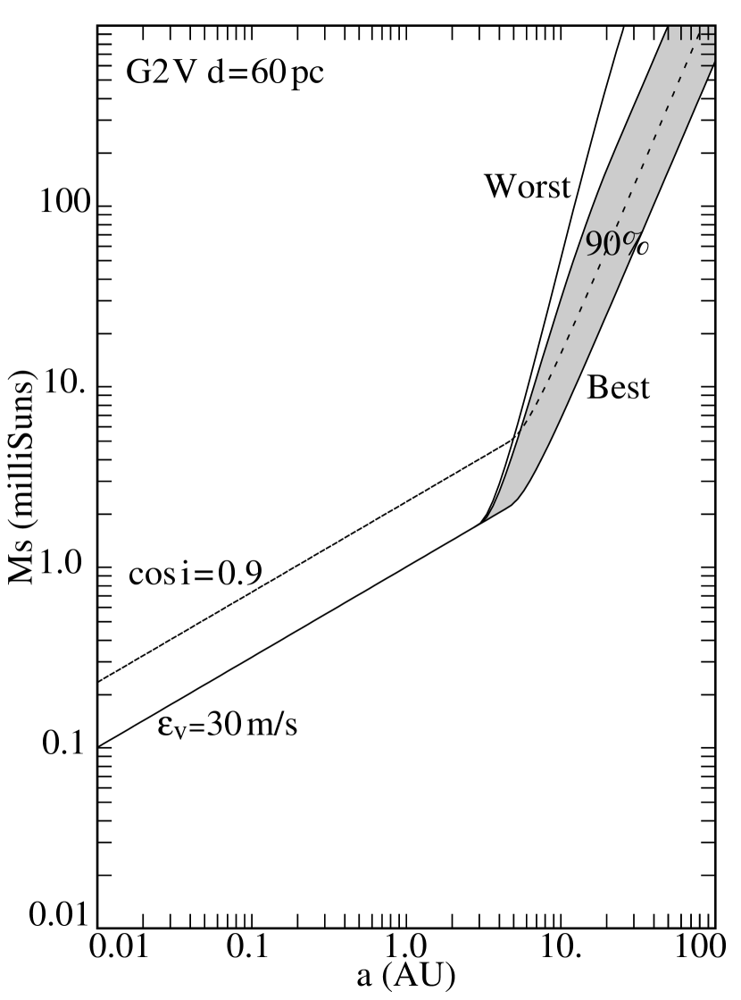
Figure 1: Radial velocity detection of companions as a function of secondary mass and total separation. The case of G dwarfs at 60 pc is taken for illustration with a velocity sensitivity ($3\sigma$) of 30 m s^-1 assumed. For periods longer than $\Delta t_{p}=5$ years we show the effects of phase in orbit including nodal passage (“Best”), quadrature passage (“Worst”) and, by shading, the range for 90% detection assuming a uniform distribution of phases. These are for edge-on systems. The dashed line indicates the range for detection at the 90% level assuming a random orientation of orbital planes. (Beyond 5 years, this is for the “Best” case only). In all cases, systems with parameters to the upper left are predicted to be detectable.

However, the problem is to detect a certain fraction of systems, not all, and it is elementary to calculate the radial velocity limits which will detect, say, 90% of the systems. An example of this calculation is shown in Fig. 1 where we use the parameters we adopt for the case of a nearby dG population. “Best” and “Worst” cases in the sense used here are shown by solid lines. The region that would encompass 90% of the systems, assuming they are uniformly distributed in phase, is shaded.

2.1.4 Inclination

All this assumes the orbit is edge-on, i.e., $i=\pm 90^{\circ}$. Inclination effects are always present. However, if orbital angular momenta vectors are distributed uniformly over the sky, probably a good assumption, then inclinations are distributed as $f(i)=\sin i$ and the chances of seeing systems face on are very low. In Fig. 1 we show with a dashed line the locus that would allow detection of 90% of the systems assuming the inclinations are distributed as above. Interestingly, for long period systems, orbital phase effects are much more important, at least at the 90% detection level.

2.2 Astrometric “Noise”

Next, we need to define exactly what will produce an erroneous positional measurement in the context of the Grid. For the ideal Grid member, specifying the position, proper motion and parallax will define its location at any epoch. To the extent that binary motions change positions in ways that cannot be modeled so simply, duplicity introduces errors into the Grid.

When these unmodeled motions exceed a certain maximum, the object will probably be rejected as a Grid member. This decision will in most likelihood be made at the end of the mission, not allowing any remediation (but see below for one proposal to soften this circumstance). Since a certain minimum number of acceptable Grid members (of order 4) must be present in any 15^∘ “Field of Regard” (FoR), redundancy must be provided in the original Grid membership. To prevent any FoR from dropping below the critical number of usable Grid members, the multiplier to provide the redundancy can be fairly large (cf., Wade, 2000) and correspondingly costly in terms of observing time.

Since astrometric measurements are fundamentally two dimensional, unmodeled motions can be present in either coordinate or shared between them. For our purposes we consider the largest component of any error, regardless of how it is projected in the observational coordinate frame.

Here and in the simulations below, we remove only linear terms from the binary motions. In particular, we do not model the parallax term. This will produce a significant modeling error only for systems with periods close to one year, since the Grid will be observed much more frequently than twice a year and over at least 5 years. As a result, the aliasing will be confined to a small region in parameter space. And, since the effect of adding a parallax term would be to absorb binary system motions that cannot be modeled by the linear terms provided (at the price of reduced parallax accuracy), we will tend to report more astrometric instability than would be observed in practice. Again, we expect the effect to be very small.

2.2.1 Face-On Systems

For circular systems the “Curvature Noise” (unmodeled astrometric motions) analysis follows Hajian et al. (1999) and is illustrated in Fig. 2 for the face-on case. Here, orbital motion causes displacements in both $x$ and $y$ coordinates. Over a finite time interval corresponding to a range in orbital phase of $2\theta$ as shown, the $y$ displacement returns to its starting point, requiring no linear motion term be removed. Anticipating our discussion of the edge-on situation, we refer to this as the “Worst” astrometric case in the sense it produces the largest unmodeled displacements.

For this case

$$2\varepsilon_{y}=a_{p}-l=\left\{\begin{array}[]{r@{,\quad}l}2a_{p}&P<\Delta t_{m}\\ a_{p}[1-\cos\frac{\pi\Delta t_{m}}{P}]&P\geq\Delta t_{m}\end{array}\right.$$ (7)

where $\Delta t_{m}$ is the mission lifetime, nominally 5 years. For long periods this becomes to first order

$$\varepsilon_{y}\sim a_{p}\left(\frac{\pi\Delta t_{m}}{2P}\right)^{2}=\left(\frac{\pi\Delta t_{m}}{2}\right)^{2}\frac{m_{s}}{a^{2}}.$$ (8)

The $x$ component involves a net translation. The difference between this and a linear translation is the noise term. The geometry is shown in Fig. 3 where the error term is the difference between an average linear motion and the projected uniform angular motion. Again, $2\theta$ will be traversed in the mission lifetime while $\vartheta$ corresponds to a specific epoch:

$$2\theta=\frac{2\pi\Delta t_{m}}{P},\quad\vartheta=\frac{2\pi(t-t_{0})}{P}.$$ (9)

From the construction we see that the apparent difference from uniform motion is

$$\Delta x(\vartheta)=a_{p}\left\{\sin\theta-\sin(\theta-\vartheta)-\frac{\sin\theta}{\theta}\vartheta\right\}$$ (10)

Extrema occur at

$$(\vartheta-\theta)_{max}=\pm\cos^{-1}\left[\frac{\sin\theta}{\theta}\right].$$ (11)

Substituting these we find

$$\varepsilon_{x}=\left\{\begin{array}[]{r@{,\quad}l}a_{p}&P<\Delta t_{m}\\ a_{p}\left\{\frac{\sin\theta}{\theta}\cos^{-1}\left(\frac{\sin\theta}{\theta}\right)-\sin\left[\cos^{-1}\left(\frac{\sin\theta}{\theta}\right)\right]\right\}&P\geq\Delta t_{m}.\end{array}\right.$$ (12)

At large periods the latter becomes

$$\varepsilon_{x}\sim\frac{a_{p}\theta^{3}}{9\sqrt{3}}=\left(\frac{\pi\Delta t_{m}}{9\sqrt{3}}\right)^{3}[m_{p}(1+q)]^{1/2}\frac{m_{s}}{a^{7/2}}.$$ (13)

Note that asymptotically the ratio of Best (i.e., $x$ component) to Worst cases becomes $\varepsilon_{x}/\varepsilon_{y}=4\pi\Delta t_{m}/9\sqrt{3}P\sim 0.8\Delta t_{m}$. The numerical factor differs by less than 3% from the corresponding ratio in the radial velocity calculation, above.

2.2.2 Edge-on Case

As for radial velocities, the orbital phase, the angular distance of the primary from the line of nodes, determines the magnitude of the astrometric noise. As can be seen in Figs. 2 and 3, inclining the system about the $x$ axis projects away the Worst of the astrometric noise, leaving the Best component intact. Exactly the opposite happens when projecting the system about the $y$ axis which removes the smaller, Best, component, leaving the Worst undiminished. Since asymptotically the Best to Worst ratio has essentially the same numerical factor as for radial velocity detection and because we assume the preparatory period, $\Delta t_{p}$ is the same as the nominal mission, $\Delta t_{m}$, that is 5 years, the dependence of the astrometric noise on orbital phase closely tracks that of the extremes in the radial velocity sensitivity, including the area required for, say, 90% detection. For clarity in the figures below, we shade those limits only for radial velocity detection.

2.2.3 Finite Inclination

While in the edge-on case the estimation of astrometric noise and its dependence on orbital phase closely parallels that of radial velocity sensitivity, that is not true for inclination effects. When the line of nodes corresponds to the $x$ axis and the largest component of the astrometric noise has been projected away, small deviations from an exact edge-on orientation can easily restore that component to the point that it dominates the error contribution. For example, in the long period case, when the ratio $\varepsilon_{x}/\varepsilon_{y}=0.1$, that is, when the period is 40.3 yr (for a mission of 5 years) or $a=11.7$ AU (in the $m_{s}=0$ limit), if the line of nodes is along the $x$ axis, the projected (Worst) component will still be larger than the Best for $\cos i\geq 0.1$, which will occur in 90% of the systems.

Combining the effects of random orbital phases and system orientations in estimating radial velocity sensitivity has the effect of broadening the 90% detection region, that is, of moving it farther to the left in Fig. 1. In contrast, combining these two effects in estimating astrometric noise pushes the left boundary of the 90% detection region toward the right, asymptotically toward the Worst locus.

As a result a reasonable “rule of thumb” for estimating the fraction of astrometric variables missed when using radial velocity prefiltering would be to compare the least sensitive limit of radial velocity detection against the largest possible component of astrometric noise when considering periods well larger than the preparatory time interval and the mission lifetime.

3 THE FILTERING PROBLEM

We consider two archetypical populations from which Grid members could be choosen. The first are G dwarfs like the Sun, but nominally at 60 pc. These objects would have $V=8.6$ mag and angular diameters of order 155 $\mu\mbox{as}$. The second are weak lined (i.e., Pop II) K giants with $\mbox{[Fe/H]}\sim-1.0$ and $M_{V}\sim-1$ mag. Estimates of SIM’s target-to-target setting time corresponds roughly to the time required to accumulate $10^{7}$ photons on a $V=12$ mag object, which we take as an approximate faint limit for a Grid object. This would place an $M_{V}=-1$ mag object at about 4 kpc (with no extinction). These objects would have angular diameters of order 20 $\mu\mbox{as}$. (We consider only the “high galactic latitude problem” for the K giants, i.e., no extinction, and comment on the problems of low latitude Grid objects, and the effects of lower luminosity objects at high latitude in the discussion).

The angular diameters are important. A simple estimate is that starspot induced positional noise could be kept below 2 $\mu\mbox{as}$ if photometric variability is kept below $\Delta V=0.05$ and 0.40 mag, respectively, for these two populations which, while not trivial, is easily achieved in practice (cf., Fekel & Henry, 1998).

3.1 Observational Screening

3.1.1 Radial Velocities

For radial velocity screening, defining the required measurement precision is critical. While more precision results in better screening for companions, this comes at a price in observing time, with the gKw’s potentially quite costly. By now we have a substantial base of experience in scrutinizing dG’s. Cumming, Marcy, & Butler (1999) summarize the current practice for these objects. We adopt a ($3\sigma$) requirement of 30 m s^-1 per observation for the G dwarfs.

The literature is less extensive regarding the K giants, not to mention the older populations. Hatzes & Cochran (1998) (also see Frink et al., 2001) indicate that, while the gK photospheres seem to be intrinsicly noisier than dwarfs, it is rare to encounter amplitudes of 100 m s^-1 (and some of that detected velocity variability might be due to multiplicity). We adopt as realistic a ($3\sigma$) detection limit of 100 m s^-1.

3.1.2 Direct Imaging

In addition to velocity screening it is possible to detect multiplicity in the wider systems through direct imaging. For main sequence primaries, there is an advantage in looking in the near infrared since secondaries, presumably also on the main sequence, will be redder, reducing the dynamic range involved. Fortuitously, the practice of adaptive optics is advancing faster at those wavelengths, offering higher spatial resolution at $2\,\micron$. This has been exploited for example by Patience et al. (1998) in detecting close companions in the Hyades using the 10 m Keck instruments.

From this we conclude that companions as faint as $\Delta K\sim 5.5$ at separations of 1″ or more should be detectable. Judging by the error estimates (Patience et al., 1998), the sensitivity declines somewhat to $\Delta K\sim 4.0$ at 0 $\farcs$2. From there we assume detectability declines steadily to $\Delta K~{}0.0$ at 0 $\farcs$02, half the diffraction limit of a 10 meter telescope at K. In applying these detection criteria, we linearily interpolate the above limits in log-separation versus magnitude and assume direct detection is impossible at separations less than 0 $\farcs$02.

3.1.3 SIM

We also consider how SIM itself can provide one last pass at catching problem systems. This has been partially described in Liu & Peterson (2000) and in detail in Liu & Peterson (2002). The idea stems from a suggestion by Wielen (1996) that companions would induce wavelength dependent offsets in position to the extent there were color differences between the two components. The situation is more complicated in an interferometer, the extent to which the overlapping wavetrains interfere determines not only the amplitude but also the sign of the offset, and this changes with wavelength whether or not there are color differences.

This filter would be applied by carefully analyzing the initial observations by SIM of each Grid member. Catching additional problem systems with the initial observations and and eliminating them from routine Grid observations could allow the Grid to start with unnecessary redundancy that could be pared down at the earliest stages of the mission.

Since it is difficult to simply characterize this type of filtering, we model it explicitly and defer discussion until its application in the Grid simulations below. At that point we will assume that each observation collects $10^{7}$ photons (i.e., the signal obtained in 2 minutes for a $V=12$ object, as mentioned above) and then evaluate whether the companion will be detected.

3.2 Parameters Space Sampled

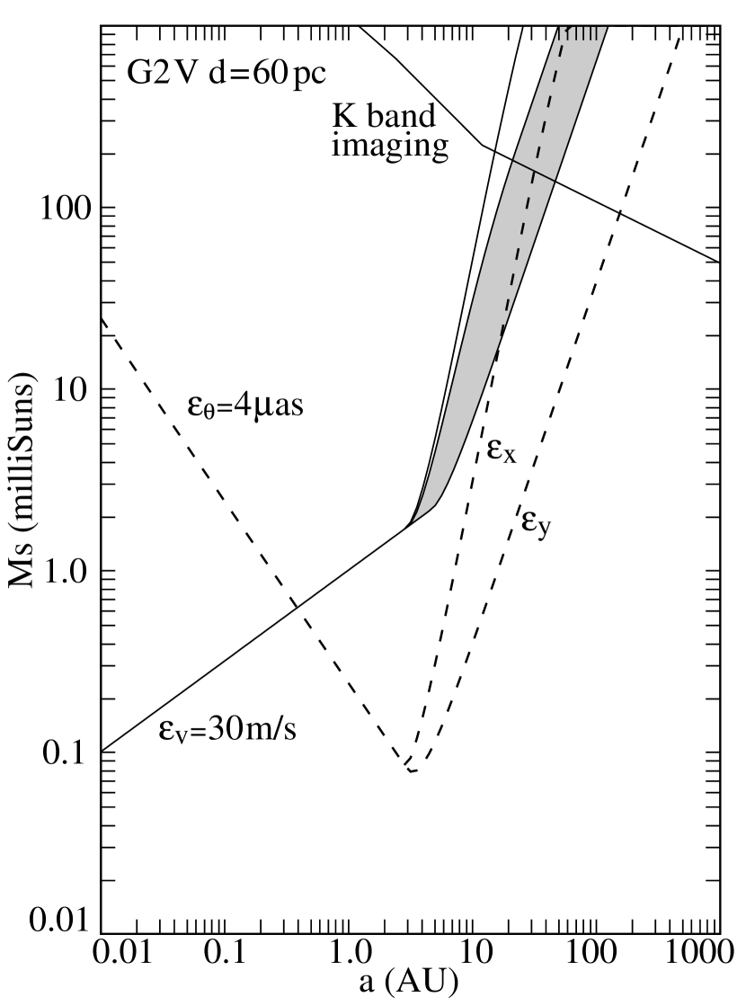
Figure 4: This shows which nearby binaries with G dwarf primaries can be detected with 30 ms^-1 radial velocity sensitivity ($\epsilon_{V}$) versus which among the same systems would be astrometrically “noisy” at the $4\,\mu\mbox{as}$ level ($\epsilon_{\theta}$). The region where K-band imaging could detect a companion is also shown. The extreme orbital phase effects are shown in both cases (at quadrature - rightmost - and at conjunction - leftmost - for radial velocity detection, and along - $\epsilon_{x}$ - and perpendicular to - $\epsilon_{y}$ - the line of nodes for astrometric detection). With regard to orbital phase, the region that would provide 90% velocity detection is shaded. An essentially identical region holds for astrometric detection and is not shown here for clarity. Systems below and to the right of the $\epsilon_{V}$ locus would not be detected by radial velocity screening. Systems above the $\epsilon_{\theta}$ locus would produce unmodeled astrometric motions of 4 $\mu\mbox{as}$ or greater.

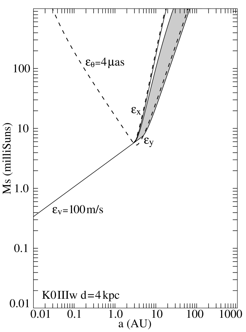
Figure 5: The same as in Fig. 4, only for 4 kpc distant weak-line K giants. Here, K-band imaging no longer contributes. A substantially reduced requirement on the radial velocity screening ($\epsilon_{V}=100$ m/s) is applied. Nevertheless, relatively few systems displaying unmodelled astrometric motions with semiamplitudes in excess of $4\,\mu\mbox{as}$ (above the $\epsilon_{\theta}$ locus) would escape radial velocity detection (below and to the right of the $\epsilon_{V}$ locus).

Figs. 4 and 5 show the limits of radial velocity binary detection compared to the regions occupied by astrometrically “noisy” systems for the two populations being considered here. Objects above and to the left of the “$\varepsilon_{v}=30$ ms^-1” and “$\varepsilon_{v}=100$ ms^-1” loci will be detected as binaries. The effects of location in the orbit are indicated as described above. Also included in these figures are the “Best” ($\varepsilon_{x}$) and “Worst” ($\varepsilon_{y}$) astrometric noise cases that would be generated by these systems, labeled as “$\varepsilon_{\theta}=4\,\mu\mbox{as}$”. Systems with parameters above these loci would exhibit 4 $\mu\mbox{as}$ or more of unmodeled motion, depending on inclination and orbital phase. The region below and to the right of the radial velocity loci, but above the astrometric loci contains systems with potentially large unmodeled astrometric motions, undetectable by radial velocity surveys of that precision.

Fig. 4 in addition shows the region of parameter space where secondaries will be detectable by imaging methods. In this figure we assume the separation is the projected separation. K-band imaging has no application in the case of the K giants. There, the brightest secondaries are assumed to be main sequence stars of just below 1 $M_{\sun}$, that is G stars that are even fainter compared to their primary at $2\,\mu m$ then they are in the visible. For G dwarf primaries K-band imaging is effective at detecting the long period companions with mass ratios above about $q=0.1$.

The differences between these two cases are striking. The G dwarfs are much more likely to be undetectable binaries, even with the help of direct imaging. However, the K giants are not completely immune to these problems. A note of caution in interpreting these figures: as we argue below, secondary masses tend to be uniformily distributed (at least for unevolved secondaries). Plotting the log of the secondary mass results in there being a large fraction of the graphed area where companions are relatively uncommon.

However, a uniform distribution of mass ratios may not adequately describe the situation at substellar masses. A large number of spectroscopic detections of companions to nearby solar type stars have been recently reported with minimum masses in the neighborhood of a few milliSuns (cf., Cumming, Marcy, & Butler, 1999). If this closely reflects the true masses of the companions, then there may well be a population of objects toward the bottom of Fig. 4 that can contribute significant astrometric noise. Systems with distant gKw primaries would be immune to the problems created by this population.

4 DISTRIBUTION OF ORBITAL PARAMETERS

4.1 The Physical Parameters

There is an extensive literature documenting efforts to deduce the statistical distributions of the various parameters characterizing binary systems. Probably the most extensive recent such effort is that of Duquennoy & Mayor (hereafter DM) and colleagues (Duquennoy & Mayor, 1991; Mazeh et al., 1992; Hogeveen, 1992), whose results we adopt as our base set of distributions.

The three parameters of physical significance are the separation, the eccentricity and the mass ratio, with the period a possible substitute for the first through Kepler’s third law. For solar type primaries a careful discussion led DM to conclude that the mass ratio is approximately uniformly distributed over the range $1\geq q\geq 0$. DM further concluded that the eccentricity distribution was consistent with the probability density function $f(e)=2e$ which is expected from energy equipartition arguments (cf., Heggie, 1975).

The remaining critical relation is the distribution of periods. DM adopted a broad Gaussian approximation to the log P distribution they found. In this work we have elected to work with the distribution of separations which is equivalent and which Heacox (1996) has shown yields the same functional form as for the periods, the only assumption being that the masses are distributed independently of these parameters, an assumption we adopt. The variation in the probability density function found by DM over the range of periods of interest is very shallow and Heacox (1996) has emphasized the small deviation of this law from the simple power law, $f(P)\sim P^{-1}$ (or equivalently, $f(a)\sim a^{-1}$). Because we will later consider a substantially more peaked distribution as an alternative, we deviate slightly from DM here and adopt a pdf for separation that is uniform in $\log a$.

There is still considerable uncertainty in these distributions and the possibility of significant variability depending on environment, age, etc. We therefore consider representative alternate density functions for these three variables. This will give us some sense of the robustness of our results to the choice of those distributions.

Recently Quist & Lindegren (2000) (hereafter QL) have used the HIPPARCOS results to constrain binary frequencies in the critical interval $0\leq\log a\leq 2$, a range particularly difficult for both spectroscopic and direct imaging at the distances of the typical HIPPARCOS objects. They concluded that the distributions adopted by DM for both separation and mass ratio did not adequately describe the HIPPARCOS detections and argued that the distribution for $\log a$ was much more sharply peaked than proposed by DM (but peaked at about the same separations) and that the mass ratio distribution increases substantially toward small mass ratios. We therefore adopt the following as the alternatives (to the pdf’s adopted by DM) for the semi-major axis and the mass ratio:

$$f(\log a)=\frac{c}{\sqrt{2\pi}}\exp-\left(\frac{(\log a-1.5)^{2}}{2}\right);\quad-2\leq\log a\leq 3$$ (14)

$$f(q)=2(1-q);\quad 0\leq q\leq 1.$$ (15)

In practice, the lower separation limit is never quite reached since we limit the inner radius to $4R_{\hbox{star}}$, which even in the case of the Sun is about 0.02 AU.

There are well known observational biases that make it difficult to extract the probability density function for eccentricity. We argue that the data presented by DM are no stronger than “consistent” with the functional form of the eccentricity density function they adopted. On the other hand the binaries in well studied clusters like the Hyades (cf., Peterson & Solensky, 1988; Patience et al., 1998) support a uniform distribution of eccentricities (although neither set of authors made that argument). We shall therefore adopt a uniform density function for eccentricity as the alternative pdf.

In general we assume that these three parameters, as well as the others described below, are statistically independent. We know that this cannot be true in the limits of very small and very large separations. In both cases there must be fewer large eccentricity cases than otherwise. For small separations, large eccentricities would take the secondary into the primary, while for large separations, large eccentricity orbits would be more easily tidally disrupted. We ignore the latter because we will be considering only relatively modest maximum separations.

For small separations a combination of the details of the processes leading to the birth of a binary and the subsequent effects of tides lead to a substantial deficit of high eccentricity systems. To allow for these effects we limit the range of eccentricities for short period G-dwarf systems by requiring that the periastron separation be no less $4R_{\hbox{star}}$. Fortunately, the results of the simulations described below are unaffected by the details of this perscription, since essentially all such systems are detected according to the criteria we have described.

The correlation of eccentricity and separation at short periods is more complicated in the case of K giants, which we discuss next.

4.2 Weak Line K Giants

The above apply explicitly to disk F and G dwarfs, by far the most extensively studied group in terms of binary parameters. The situation for gKw stars is poorly documented by comparison. However, we believe that we can, with care, extend the results described above to these objects. The critical fact on which the assumption hinges is the discovery by Latham and coworkers (Carney, et al., 1994, Latham 2000, private communication, Latham, et al. 2002) that the binary frequency in the F and G subdwarfs is indistinguishable from that of disk G dwarfs. That in stark contrast to the long held belief that Pop II objects had about half the number of binaries compared to Pop I. Latham et al. (2002) also provide evidence that the mass ratio distributions for the two populations are similiar.

By far the most critical parameter in comparing binary populations is their frequency. Finding that the two populations have the same binary frequency, it is not a large leap to argue that the other pdf’s are probably quite similar as well (save, perhaps, for more complete tidal stripping, which does not affect us). We adopt that hypothesis and assume that binaries are basically the same, whether formed 10 Gyr or 100 Myr ago.

However, we are not dealing with main sequence G primaries, but K giants. Evolution off the main sequence will certainly have a significant effect if for no other reason than that the primaries will have radii approaching 30 $R_{\sun}$, $\log a=-0.85$. Further, it is not at all clear that the K giant that is now the primary, was the primary of the original system of main sequence objects; we allow for the possibility of more than one evolutionary channel for creating binaries with a K giant primary. We consider simple evolutionary effects first.

4.2.1 Evolution of the primary

The first channel we consider for creating binaries with a K giant primary is that of simple first time evolution of the original primary toward the giant branch. Specifically we assume we are dealing with an object that is 10 Gyr old and nominally 1 $M_{\sun}$. We also assume the secondary is then at least slightly below that mass and is still on the main sequence.

We do not deal here with the case of a system consisting of two giants (i.e.,very small mass differences). Such systems are not all that uncommon, judging by their frequency in the Bright Star Catalogue (Hoffleit & Jaschek, 1982) for example. However, they are easily recognized and will be rejected from the Grid immediately. Further, their apparently high frequency is in part the result of the relative brightness of the system compared to a single giant; the volume probed by a magnitude limited catalog such as the BSC for such systems approaches a factor of three larger than that for systems dominated by the primary. Since such systems require mass ratios quite close to unity, their true frequency is small and ignoring them will have no effect on our conclusions.

The effect of simple evolution of the primary will be to disrupt the binary in those systems with initial separations less than about twice the final radius of the primary. Such systems will in general not produce a simple field K giant and we discard them when such parameters are generated in the Monte Carlo simulations. For slightly wider systems there will be a range of separations where initially eccentric systems will undergo partial or complete circularization.

The calculation we adopt is slightly more complicated, and we proceed as follows. First, with the distance for the adopted absolute visual magnitude (dependent on the metal deficiency) for the K giant and the angular diameter from van Belle (1999) appropriate to the color of a K0 III, we calculate the primary’s radius. Then, if initially periastron is less than 4 stellar radii we alter the eccentricity and separation, conserving angular momentum (Nelson & Eggleton, 2001), so that periastron is $4R_{\hbox{star}}$ or, if that is not possible, the orbit is circular. In the latter case we then check whether the primary is within its Roche lobe (Eggelton, 1983, but beware, Eggleton’s “$q$” is our $q^{-1}$). If not, the system is rejected.

The upper limit on separation is maintained at $\log a=3$.

4.2.2 K giant secondaries

On review of the various modes of binary evolution, one other channel appears to provide a significant number of binary systems with K giant primaries, although here the secondary, a white dwarf, was the system’s original primary.

In order for the original secondary to have evolved to a metal deficient K giant, we argue that it must have been nominally 1 $M_{\sun}$. For the sake of this calculation we assume that all metal poor stars are about 10 Gyr old and are coeval. Further, we assume that it is highly unlikely that the original secondary was significantly less than 1 $M_{\sun}$ and then received just the amount of mass from the evolving primary to make it enough more massive than 1 $M_{\sun}$ that it evolved into the giant phase now. The original secondary will be taken as having been 1 $M_{\sun}$ all along.

Generalizing this argument, we assume that if there were any significant mass transfer as the primary evolved it would not produce a system that contains a Pop II K giant now. This implies that we are dealing with systems with separations of 10 AU or more. While approximate, this cutoff is uncertain by no more than a factor of two, which is tolerable given the small contribution of this channel.

Given these assumptions, we know that for Pop I an isolated star will evolve to a white dwarf if it is initially 8 $M_{\sun}$ or less (the alternative, a more massive star going supernova, is a negligible source of K giant systems). In binaries where the primary can be stripped of its hydrogen envelope at an early stage the lower mass limit for forming neutron stars may be considerably higher, perhaps up to 12 $M_{\sun}$. However, the mass functions are sufficiently steep that the upper limit to masses contributing white dwarf secondaries has almost no effect on the results. We take 8 $M_{\sun}$ as the upper mass limit and adopt it for Pop II objects as well.

Over the range $1\,\mbox{$M_{\sun}$}\leq m_{i}\leq 8\,\mbox{$M_{\sun}$}$ the primary loses mass becoming a white dwarf of mass $m_{f}$. We adopt a simple power law to describe the outcome,

$$m_{f}=0.6m_{i}^{0.42},$$ (16)

which gives a Chandrasekar mass white dwarf for an 8 $M_{\sun}$ primary and a 0.6 $M_{\sun}$ white dwarf for a 1 $M_{\sun}$ primary, as derived for typical field white dwarfs. We further assume that the frequency of primary masses follows the Salpeter mass function and the mass ratio is uniformly distributed in the original, unevolved binary.

The ratio of the number of systems from this second channel is related to the number in the first channel (K giant primary) through the mass function. For the second channel the number density function of primaries with mass, $m_{p}\pm dm_{p}$ and secondaries with mass ratio, $q\pm dq$, is given by

$$dn=\phi(m_{p},q)dm_{p}dq=km_{p}^{-2.35}dm_{p}dq,$$ (17)

where the constant $k$ is for normalization. We convert this to a distribution of the secondary mass and integrate over primary masses of 1 to 8 $M_{\sun}$ to obtain:

$$\Delta n_{s}=0.42kdm_{s}.$$ (18)

In turn, when the K giant is the original primary, then from the same mass function we find for the first channel (a 1 $M_{\sun}$ K giant)

$$\Delta n_{p}=kdm_{p}.$$ (19)

Equating $dm_{p}$ from the normal channel to $dm_{s}$ for the white dwarf channel we find

$$dn(wd)/dn(normal)=0.42.$$ (20)

(This ratio is sensitive to the mass ratio distribution. Substituting the linearly increasing function proposed by QL for example, the above evaluates to 0.25).

We must account for discarding the close systems (those that undergo mass transfer) from the white dwarf channel. In terms of the nominal distributions, the relevant one being the uniformly distributed $\log a$, $-2\leq\log a\leq 3$, only 40% of the original systems survive ($a\geq 10\,$AU) and the ratio above is reduced to 0.17 (or 0.10 for the linear mass ratio pdf). (Using the more sharply peaked distribution for separations found by QL, the fraction of acceptable systems increases to 67% and the ratio of the two channels increases to 0.28. Interestingly, if both of the QL distributions, mass ratio and separation, are adopted the overall ratio remains at 0.17).

4.3 Geometric Parameters

In addition to these three physical parameters there are several which describe the position of the orbit in space and the phase of the orbit. There is no evidence that these are distributed in any other way than one would expect. We therefore assume that the longitude of the ascending node, $\Omega$, and the argument of periastron, $\omega$ are uniformly distributed over (0,$2\pi$) and that orbital planes are randomly oriented in space, leading to the well know pdf for inclinations, $f(i)=\sin i$. Finally, we assume each system is randomly distributed in orbital phase. That is, $t-t_{P}$ is uniformly distributed over $(0,P)$.

5 SIMULATIONS

We have run a number of Monte Carlo simulations to estimate the extent to which astrometrically unstable systems can be detected. We varied the assumed orbital parameter distributions as well as certain other parameters to illustrate how sensitive our conclusions were to the various uncertainties. Each run involves simulation of $10^{4}$ binary systems. In every case, we ran more than one such simulation, mostly to check that we would not inadvertently reproduce the results with some “$3\sigma$” values. The results quoted and graphed are those for one specific run and should be reliable at the 1% level.

The parameters of each simulated binary system were assumed to represent the state of the system at the nominal start of the mission. To assess whether the system would be detectable as a spectroscopic binary, we simply compared the velocity semi-amplitude of the system to our threshold detectivity (i.e., 30 ms^-1 for G dwarfs) if the period was shorter than the nominal 5-year preparatory time. For periods longer than 5 years we used half the total velocity change that would have taken place the previous 5 years. No allowance was made for aliasing (which can modulate detectivity significantly, but only over a small area in parameter space). Also, no attempt was made to model the radial velocity detection process – a semi-amplitude was either larger than the detection threshold, or not.

K-band detection was determined taking the nominal apparent separation and the K magnitude difference deduced from the masses and comparing them to the criteria defined above. Again, no effort was made to model the detection process in a statistical sense.

Only in the case of evaluating whether SIM would detect the presence of a companion did we make a detailed model of the detection process. This results in the occasional “detection” of a system that is unlikely to be detected, and vice versa (we refer to this as “leakage”). The effect is small and will be remarked on only briefly below.

To assess astrometric stability we also distinguished systems with periods longer than or shorter than the nominal mission life, 5 years. For shorter periods, we evaluated the nominal apparent ellipse, calling the system “unstable” if the semimajor axis exceeded $4\,\mu\mbox{as}$. For longer periods we took 20 samples, evenly spaced, of the $x$ and $y$ components of the system’s position over a mission lifetime, removed a linear term, and again looked for any residuals that exceeded $\pm 4\,\mu\mbox{as}$. We note that a semi-amplitude of $4\,\mu\mbox{as}$ is approximately $2.8\,\mu\mbox{as}$, rms.

5.1 The Circular Approximation

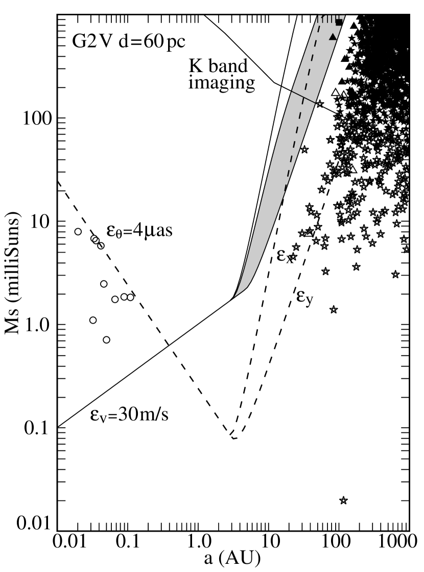
Figure 6: The astrometrically “stable” systems for $10^{4}$ simulated binaries with G2 V primaries at 60 pc, shown as a function of semimajor axis and secondary mass. The symbols indicate whether the systems would have been detected as binaries and if so, how: open circle ($\bigcirc$) for Rv only detectable, open box ($\square$) for Rv + SIM only detectable, and open triangle ($\bigtriangleup$) for SIM only detectable. Filled versions of those symbols indicate the systems would be detectable by K-band imaging, too. A filled star ($\bigstar$) indicates detectable by K-band imaging only, while an open star indicates a system undetectable by any of the techniques considered. The circular approximation does an excellent job representing the regions of astrometric stability (below the $\epsilon_{\theta}$ locus) and radial velocity detectability (above the $\epsilon_{V}$ locus).

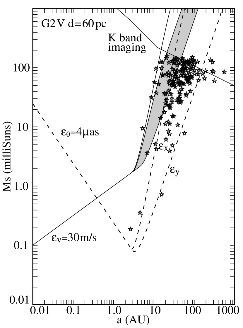
Figure 7: As for Fig. 6 only for the astrometrically unstable systems (above the $\epsilon_{\theta}$ locus) that are in principle not detectable by radial velocity screening (to the left of the $\epsilon_{V}$ locus) or K-band imaging (above and to the right of that locus).

We first compare the results from the simulations to the analytic results from the circular orbit approximation. Figures  6 and 7 show the results for the simulation for G dwarfs using the nominal distributions for astrometrically stable systems and for those unstable systems that would not be detectable using radial velocity screening and/or K-band imaging. Although the high density of plotted points somewhat obscures the boundaries in the former, it is clear that the circular orbit approximation gives a good estimate of which binary systems are detectable by radial velocity techniques and which binary systems will display deleterious unmodelled motions.

In Fig. 6 we also indicate stable systems which would in principle be detectable by K-band imaging and in Fig. 7 the sharp limits on lack of detectability of unstable systems. Here, the issue is the extent to which the semimajor axis approximates the mean separation. As can be seen, this too is an excellent approximation both in the mean (the mean separation should be about $0.95a$, cf., Leinert et al., 1993), and in the small dispersion about that mean.

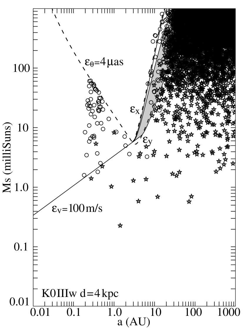
Figure 8: The weak-lined K giants that would be astrometrically stable. Symbols as in Fig. 6.

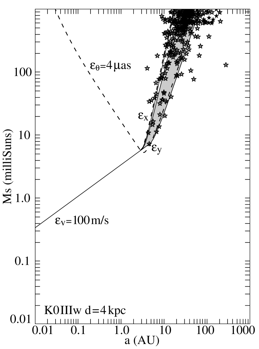
Figure 9: As for Fig. 8 only for the astrometrically unstable (above the $\epsilon_{\theta}$ locus) but radial velocity undetected (below the $\epsilon_{V}$ locus) systems. Open stars indicate undetected systems with main sequence companions and filled stars indicate such systems with white dwarf companions.

Figures 8 and 9 show the astrometrically stable and unstable, undetected systems, respectively, for the Pop II K giants. Again, the detectability and stability regions are in close agreement with the simple circular orbit predictions. As remarked earlier, the fraction of unstable but undetected systems is somewhat smaller for the K giant case. The really notable difference is the far larger fraction of stable systems in this latter case.

We next consider in more detail the simulation results for these two populations.

5.2 The G Dwarfs

The results from the individual simulations for nearby (60 pc) disk G dwarfs are given in Table 1. Column (1) gives a reference number (to identify entries in the Venn diagrams) and (2) a phrase describing the subset. The results from the simulations with various parameter distributions come next, with “nominal” (3) basically the DM (as slightly modified) choice, “$f(e)=1$” (4) for a uniform eccentricity distribution, “$\log a$” (5) for the fairly peaked semimajor axis distribution of QL, and “$q$” (6) for a distribution of mass ratios rising (linearly) to small ratios. The remaining columns are described below.

The various population subsets listed are generally “exclusive”. That is, to get the number of K-band detections with no radial velocity detections, but independent of being detectable by SIM, one adds the results of lines 13 and 14. The number of systems not detected, independent of their suitability as Grid members is found by adding lines 4 and 7, and so forth.

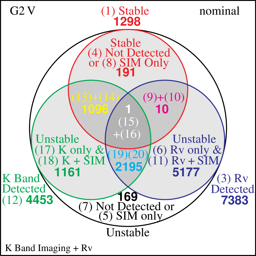
Figure 10: The Venn diagram showing the detectability of astrometrically stable and unstable systems with G2 dwarf primaries. The effectiveness of K-band imaging in combination with radial velocity screening in detecting companions is shown, independent of any contribution SIM might make. Numbers in parentheses index entries in Table 1.

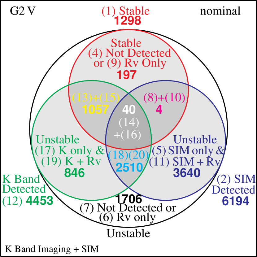
Figure 11: The Venn diagram showing the effectiveness of K-band imaging and an ultimate screening by SIM in detecting companions in systems with G2 dwarf primaries, independent of any radial velocity screening.

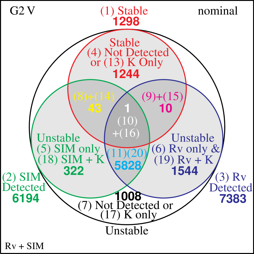
Figure 12: The Venn diagram showing the effectiveness of discerning radial velocity variations plus an ultimate screening by SIM in detecting companions in systems with G2 dwarf primaries, independent of any K-band imaging.

For the nominal distributions (column 3 of Table 1), these results are shown in Venn diagrams, Figs. 10 – 12. It is not possible to show the full overlap of stability, K-band detection, RV detection, and SIM detection simultaneously in such graphics, so we show the three possible permutations, two detection techniques at a time. We argue below that SIM probably won’t detect systems in unique parts of parameter space, compared to radial velocity screening combined with K-band imaging, and thus will concentrate on the combination presented in Fig. 10.

The situation for the dG systems is that radial velocity screening and K-band imaging combine to be remarkably efficient at detecting the presence of a companion. What is unexpected is the remarkably small fraction of systems that are astrometrically stable. This result is robust over the range of parameter distributions we consider.

Although we do not propose to get into the issue of optimizing the Grid selection process, a naive approach would be to simply throw out all systems detected as binary. In the “nominal” example, that would result in a yield of 191 stable systems and 169 unstable systems, a devastating result.

Even if one could imagine some process of deciding which detected binaries to retain from the radial velocity and K-band measurements that was 100% successful at removing the unstable systems, there would still be a $\sim 13$% contamination rate from undetected systems and a discouragingly low $\sim 13$% yield (1298 out of $10^{4}$). The latter would imply having to examine $1.5\,10^{4}$ potential targets to get a yield of 2000 Grid members.

This, of course, assumes the initial population is 100% binary, which we discuss below.

5.3 The weak-lined K giants

The situation for the K giants is summarized in Table 2, which presents basically the same breakdown of the simulation results as above. K-band imaging makes no contribution here, at least for the systems we consider, and those entries have been replace by a summary of the contribution from white dwarfs.

Again the main conclusions are most easily drawn from the Venn diagram shown in Fig. 13. Foremost is that there is the potential for a significant yield, with about 52% deemed astrometrically stable. Even the issue of how to determine which are stable seems straightforward. If one ignores detectability by SIM and simply rejects any system showing radial velocity variability, then 50% of the systems will be accepted, with only a 6% contamination rate. It is hard to see how to improve on this much.

We note that the latter result is in complete agreement with the estimate by Gould (2001), the addition of the white dwarf component does not qualitatively affect the usefulness of the gKw population for the SIM Grid. On the other hand, nearly a third of the unstable but undetected members of this population contain white dwarf secondaries.

Again, these conclusions are little affected by altering the various parameter distributions, as seen in columns 3–6 of Table 2. Gould (2001) has noted that his estimates are most sensitive to the choice of period distribution, which as noted is equivalent to the separation distribution. But we see little effect going from a pdf uniform in $\log a$, as assumed in the “nominal” simulations, and the fairly peaked distribution proposed by QL. Consequently, we conclude that in terms choosing Grid candidates, no one distribution stands out as unusually poorly defined.

5.4 The Role of SIM

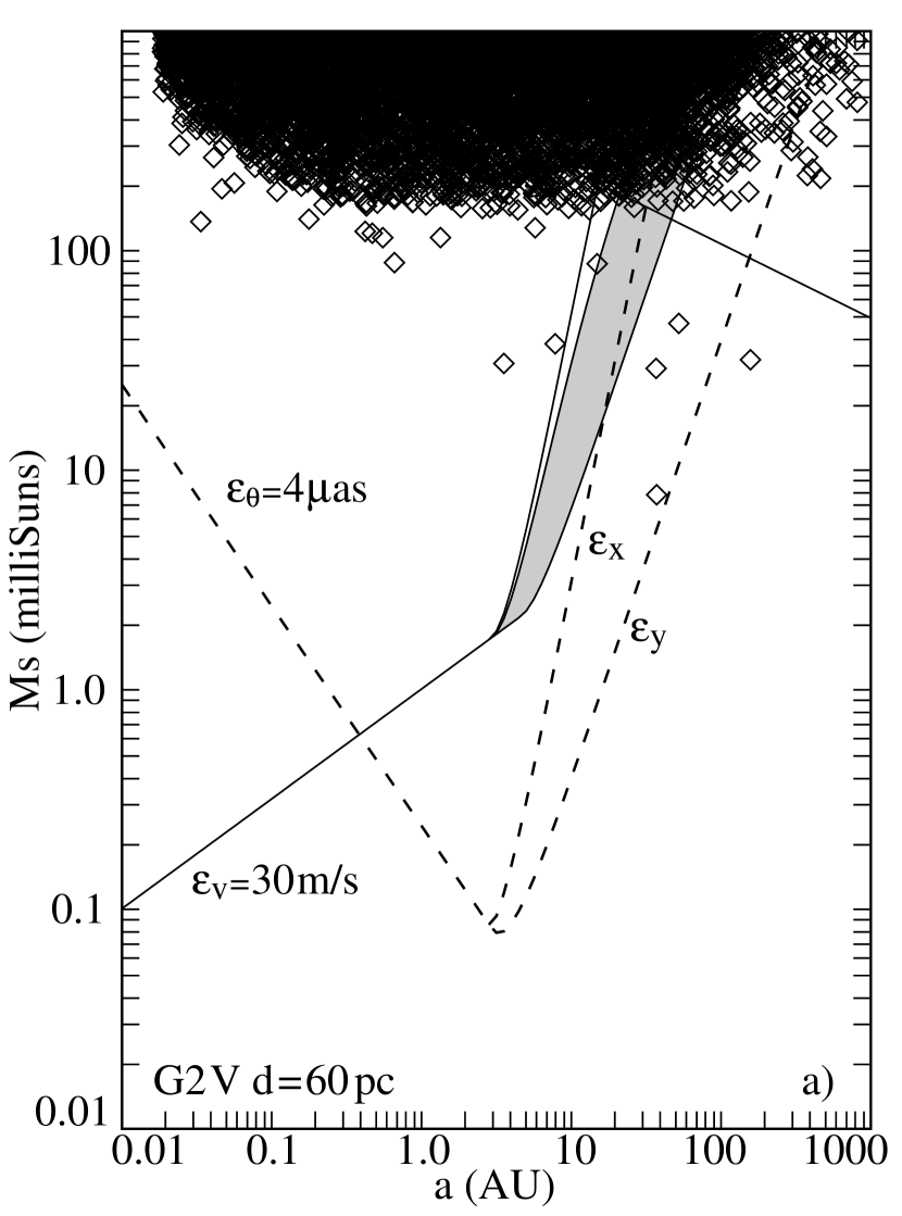
Figure 14: Shown are all systems detected by the simulation of the SIM measurement process (at the $2\sigma$ level) for a) the G dwarfs and b) the K giants. With the exception of some leakage in the measurement process, essentially all unstable systems detected by SIM are detectable using ground based methods.

As described in the Introduction, one of the goals of this investigation was to discover whether SIM, itself, could contribute a useful final screening for problem Grid members. It appears that is unlikely. In Fig. 14a we show all dG systems detected by the SIM simulation and in Fig. 14b those for the gKw systems. In the dG case, except for a little leakage in the simulation of the detection process, essentially all SIM detections are capable of being detected by either the radial velocity screening or K-band imaging. For the K giants, the coincidence of the radial velocity sensitivity limit with the limits for the onset of astrometric instability imply that few unstable systems would be detected by SIM without being detectable by Rv screening. These conclusions are borne out quantitatively in Tables 1 and 2.

That said, we note that being “detectable” and actually being “detected” are quite different matters, and that a careful examination of the SIM astrometric signal for an indication of multiplicity could materially reduce contamination due to leakage in the radial velocity screening process.

5.5 Distances and Accelerations

In assessing the weak-lined K giants we have taken as the ideal case a substantially metal weak object, of order $[Fe/H]\sim-1$ in assuming $M_{V}\sim-1$. There are many more “thick disk” giants in this apparent magnitude range than extreme Halo objects and it may on occasion be required to rely on these not-so-distant objects in parts of the Grid. To this end we have simulated the case for $M_{V}=0.5$, where the objects are still assumed to be $1\,\mbox{$M_{\sun}$}$ (or, equivalently, this shows the effects of 1.5 mag of absorption for the higher luminosity objects). The results are shown in Table 2, column 7 (“$M_{V}$”). These objects are at about 2 kpc (unreddened) and there is now a small range of separations where astrometric instability can occur without significant probability of radial velocity detection. Excluding all systems that could be detected by Rv screening, the yield drops a little (4679) and the fraction of unstable systems in the retained population rises to about 10% (488). Here it might be useful to use the wide systems as seen by SIM and eliminate the closer ones to reduce the contamination fraction.

However, there is a better way of proceeding. Jacobs (2000) has suggested that at little loss in degrees of freedom it might be possible in the post-mission, data processing phase to identify those systems that show curvature and selectively add quadratic terms to the proper motion solutions. We show in Table 2 the effect of introducing quadratic terms in two of the simulations: the “nominal” case (column 8, “2-nom”) and for the lower luminosity case just described (column 9, “$2-M_{V}$”).

The results are striking. In the nominal case we see a substantial (30%) increase in actually “stable” systems, and an even more striking 40% gain for the lower luminosity ($M_{V}=0.5$) population. More remarkably, in the practical example of simply excluding all systems detectable as radial velocity variables, we revert to the yields found previously (50% and 47%, respectively) but with miniscule (0.3% and 0.8%, respectively) contamination by unstable systems. Again, this is completely consistent with the findings of Gould (2001). Since at most 10% of the systems will benefit from this adjustment, one can expect little loss in the accuracy or numerical stability for the Grid in the data reduction.

We wondered about the sensitivity of these results to the choice of the stability requirement. How badly would the yields degrade if for example we required $2\,\mu\mbox{as}$ amplitude for “stability”? The results from several simulations showed that the yields were surprisingly insensitive to the choice of that parameter. We show in Table 2, column 10 (“$22M_{V}$”) the results for the most extreme case: lower luminosity K giants, but with quadratic terms in the proper motion solutions. The yield (everything not seen as variable in the radial velocity screening) remains the same and the contamination level rises from 0.8% (36) to 1.1%. We can expect that many areas on the sky will have Grid members stable to very high precisions, which may open additional opportunities for SIM investigators.

In Table 1, column 7 (“2-nom”) we show the extent to which introducing quadratic terms into the proper motion reductions reduce the high fraction of undetected, astrometrically unstable systems with G dwarf primaries. As with the K giants the improvement is dramatic. The number of stable systems potentially available increases by more than a factor of 2 although it remains a fairly low 31%. Further the contamination rate (lines 5 + 7) is a remarkable 0.6%. Again, we do not address exactly how to identify the stable systems, a critical step.

Finally, we wondered how strongly the selection process would degrade with reduced precision in the velocity screening and the results were again quite encouraging. For the K giants, taking the simulation with the nominal distributions, modelling only linear proper motion terms and retaining a $4\mu\mbox{as}$ stability criterion, we find that dropping the ($3\sigma$) velocity criterion to 200 ms^-1 doubled the “unstable but undetected” contamination to about 3% and increased the yield by 10% (to about 55%). As before, introducing quadratic terms in the proper motions reduced the contamination by an order of magnitude. However, this brings us into an area that we have not treated carefully, the radial velocity detection process, and we think it is premature to present details. The radial velocity detection process needs cardful modelling before we can provide a realistic estimate of the contamination rate, particularly given the very small fractions calculated here.

6 CONCLUSIONS

We have considered the question of how to choose reliable objects for SIM’s Grid, and have looked at two groups of objects, nearby ($\sim 60$ pc) disk population G dwarfs and kiloparsec distant thick disk/halo, weak-lined K giants, which have been mentioned in this context. A knowledge of binary frequency and how the parameters of binary systems are distributed is critical in answering this question. We have argued that what is currently known for nearby G stars applys generally.

However, evolutionary effects must be allowed. The K giants will have modified the orbits of close companions, or have removed them. Further, the K giant primary need not have been the original primary of the system, and we estimate the fraction that will have white dwarf companions now, the result of evolution of the original primaries, to be around 15%.

With these results we have found that the weak-lined K giants at distances of the order of 4 kpc when screened for radial velocity variations at the 100 ms^-1 level, will provide a sample of objects that will work quite acceptably for the SIM Grid. For the standard Grid data reduction, including only linear terms in the proper motions, one expects a contamination level around 6–10%, depending on the exact distance of the population. Allowing quadratic terms in the proper motions where necessary, unmodeled motions can be kept below $2\,\mu\mbox{as}$ for all but 1% of the Grid (a result first obtained by Gould (2001)).

We also considered the plausibility of using nearby G dwarfs for this purpose and argued that they are susceptible to two significant failure modes if they were to be used. First, considering the circular orbit approximation we found that there is a sizeable range at low mass ratios where companions would produce significant astrometric motions but not radial velocity variations. If the usual distributions found for more massive companions holds over the whole range, this would provide no significant channel for contamination. However, the spate of recent discoveries of Jupiter mass companions to nearby G dwarfs suggests extrapolation of those results to low masses may not be wise.

Further, even if the assumed parameter distributions are as found for the systems with stellar mass companions, we showed that if that population consists of 100% binaries, then the rejection rate from radial velocity and K-band screening will reach at least 70%, requiring the screening if a large number of potential candidates. The use of quadratic terms in the proper motion reduction would again leave almost no contamination in the resulting sample. However, up to half the Grid would require fitting these additional terms, raising questions about the effects on the Grid’s numerical stability. Critical to these concerns is the fraction of G dwarfs that are single, a parameter that is poorly known and could well be zero.

We do note that there are limitations on the use of K giants as Grid members in the Galactic plane, due to obscuration. It might be that in this reduced area, use of G dwarfs with a relatively high redundancy factor would be an acceptable alternative.

Table 1: Stability and Detectability of G2 V Binary Systems.

(1)	(2)	(3)	(4)	(5)	(6)	(7)
Index	Binary Status	nominal	$f(e)=1$	$\log a$	$q$	2-nom
1	Stable	1298	1276	1374	1550	3152
2	SIM Detected	6194	6180	6202	4772	6194
3	Rv Detected	7383	7397	6364	7136	7383
4	Stable: Not Detected	187	194	267	385	336
5	Unstable: SIM Detected only	2	4	5	4	0
6	Unstable: Rv Detected only	1539	1573	842	2628	1482
7	Unstable: Undetected	167	181	317	354	18
8	Stable: SIM only Detected	4	5	9	6	6
9	Stable: Rv only Detected	10	11	0	18	67
10	Stable: SIM + Rv only Detected	0	0	1	0	6
11	Unstable: SIM + Rv only Detected	3638	3613	1779	3038	3632
12	K Detected	4453	4419	6780	3567	4453
13	Stable: K only Detected	1057	1022	1036	1093	1895
14	Stable: K + SIM only Detected	39	43	61	48	322
15	Stable: K + Rv only Detected	0	0	0	0	4
16	Stable: K + SIM + Rv Detected	1	1	0	0	516
17	Unstable: K only Detected	841	833	1321	740	3
18	Unstable: K + SIM only Detected	320	321	620	234	37
19	Unstable: K + Rv only Detected	5	6	15	10	1
20	Unstable: K + SIM + Rv Detected	2190	2193	3727	1442	1675

Note. — Col. (1): Identifies which quantities are used towards the totals shown in Figs. 10–12. Col. (2): Indicates the (exclusive) logic used in these totals. Col. (3): A simulation based on the “nominal” probability density functions for the various binary parameters as defined in the text. Col. (4): A simulation using the “nominal” pdf’s for the binary parameters, but substituting a uniform distribution for eccentricity. Col. (5): A simulation using the “nominal” pdf’s for the binary parameters, but substituting the somewhat peaked distribution of QL for the semi-major axis. Col. (6): A simulation replacing the “nominal” uniform mass ratio (“q”) pdf with one that rises linearly toward small ratios. Col. (7): A simulation using the “nominal” pdf’s, but with quadratic terms removed from the apparent proper motions before characterizing the motions as stable or unstable.

Table 2: Stability and Detectability of K0 IIIw Binary Systems.

(1)	(2)	(3)	(4)	(5)	(6)	(7)	(8)	(9)	(10)
Index	Binary Status	nominal	$f(e)=1$	$\log a$	$q$	$M_{V}$	2-nom	2-$M_{V}$	22$M_{V}$
1	Stable	5174	4982	5220	5611	4395	6834	6124	5858
2	SIM Detected	3534	3374	3698	1734	3607	3534	3607	3607
3	Rv Detected	4988	5147	4928	4624	5321	4988	5321	5321
4	Stable: Not Detected	2908	2789	2930	3987	2556	3053	2818	2806
5	Unstable: SIM Detected Only	120	116	135	55	198	5	8	12
6	Unstable: Rv Detected Only	3116	3379	2774	3582	3400	2296	2681	2853
7	Unstable: Undetected	156	185	247	243	290	11	28	40
8	Stable: SIM Only Detected	1828	1763	1760	1091	1635	1943	1825	1821
9	Stable: Rv Only Detected	286	273	351	454	147	1106	866	694
10	Stable: SIM + Rv Only Detected	152	157	179	79	57	732	615	537
11	Unstable: SIM + Rv Only Detected	1434	1338	1624	509	1717	854	1159	1237
12	White dwarfs	1474	1411	1418	1425	1383	1474	1383	1383
13	White dwarfs: Unstable	472	442	542	433	519	115	124	161
14	WD: Unstable + Undetected	59	74	82	57	115	2	5	5

Note. — Col. (1): Identifies the quantities shown in Fig. 13. Col. (2): Indicates the (exclusive) logic used in these totals. Col. (3): A simulation based on the “nominal” probability density functions for the various binary parameters as defined in the text. Col. (4): A simulation using the “nominal” pdf’s for the binary parameters, but substituting a uniform distribution for eccentricity. Col. (5): A simulation using the “nominal” pdf’s for the binary parameters, but substituting the somewhat peaked distribution of QL for the semi-major axis. Col. (6): A simulation replacing the “nominal” uniform pdf for mass ratio (“q”) with one that rises linearly toward small ratios. Col. (7): A simulation using the “nominal” pdf’s but assuming $M_{V}=0.5$ (d = 2 kpc). Col. (8): A simulation using the “nominal” pdf’s and $M_{V}=-1$, but with quadratic terms removed from the apparent proper motions before characterizing the motions as stable or unstable. Col. (9): A simulation combining the use of quadratic terms in the proper motions and the lower luminosity assumption of Cols. (7) & (8). Col. (10): A simulation with the same assumptions and distributions as Col. (9), but increasing the astrometric requirement to 2 $\mu\mbox{as}$.

Figure 2: The astrometric “Worst” case. The motion along the $y$ axis has no linear component to remove, we equate the amplitude to twice the maximum allowable noise, $\varepsilon_{y}$.

Figure 3: The astrometric “Best” case. Uniform linear motion differs from projected uniform circular motion by third order terms. The linear motion has been exaggerated for illustration.

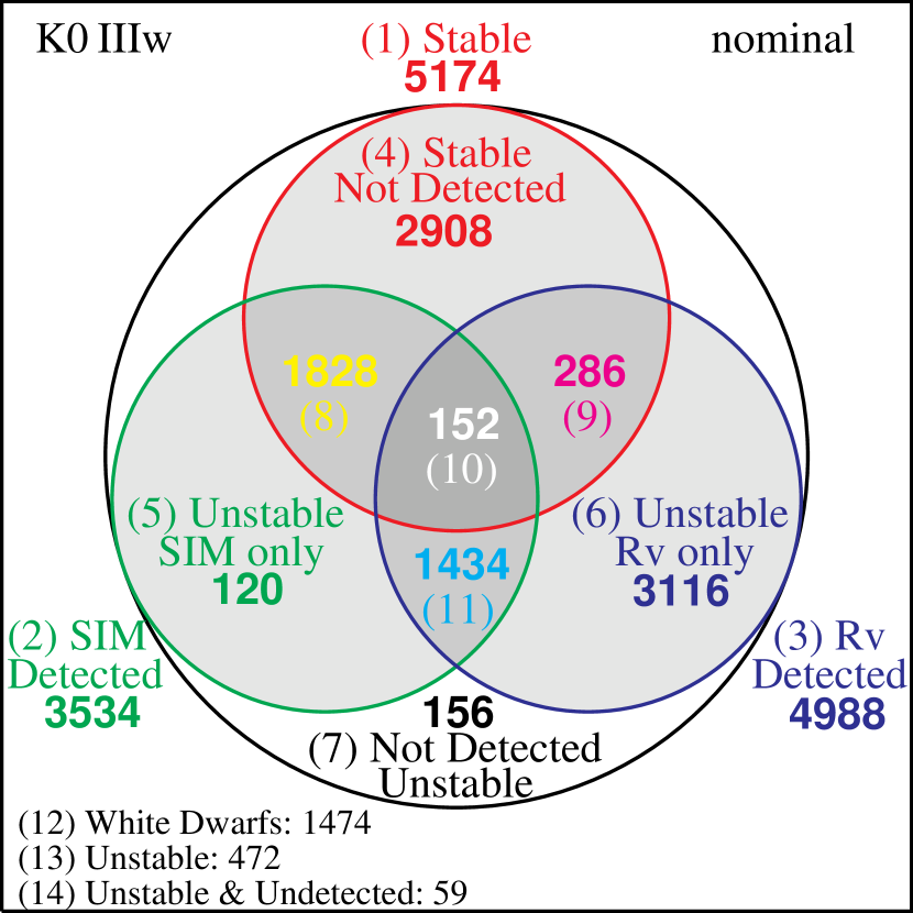
Figure 13: The Venn diagram for systems with weak-lined K giant primaries showing the dectability of a companion with SIM and radial velocity screening and their overlap. Numbers in parentheses index entries in Table 2. The contributions from systems with white dwarf companions are summarized at the lower left.

References

- Boden, Unwin & Shao (1997) Boden, A., Unwin, S. & Shao, M. 1997, in Hipparcos Venice ’97, ed B. Battrick (ESA SP-402) (Noordwijk: ESA), 789
- Carney, et al. (1994) Carney, B.W., Latham, D.W., Laird, J.B. & Aguilar, L.A. 1994, AJ, 107, 2240
- Cumming, Marcy, & Butler (1999) Cumming, A., Marcy, G.W., & Butler, R.P. 1999, ApJ, 526, 890
- Danner, Unwin & Allen (1999) Danner, R., Unwin, S., & Allen, R.J. 1999, SIM Space Interferometry Mission: Taking the Measure of the Universe (JPL 400-811; Washington: NASA)
- Duquennoy & Mayor (1991) Duquennoy, A. & Mayor, M. 1991, A&A, 248, 485 (DM)
- Eggelton (1983) Eggleton, P.P. 1983, ApJ, 268, 368
- Fekel & Henry (1998) Fekel, F. & Henry, T. 1998, in ASP Conf. Ser. 154, The 10th Cambridge Workshop on Cool Stars, Stellar Systems and the Sun, eds R.A. Donahue & J.A. Bookbinder, (San Francisco: ASP), 755
- Frink et al. (2001) Frink, S., Quirrenbach, A., Fischer, D. Röser, S., & Schilbach, E. 2001, PASP, 113, 173
- Gould (2001) Gould, A. 2001, ApJ, 559, 484
- Hajian et al. (1999) Hajian, A.J., Mason, B.D., Corbin, T.E., & Seidelmann, P.K. 1999, in “Analysis of K Giants for the SIM Grid Star List”, privately circulated
- Hatzes & Cochran (1998) Hatzes, A.P. & Cochran, W.D. 1998, in ASP Conf. Ser. 154, The 10th Cambridge Workshop on Cool Stars, Stellar Systems and the Sun, eds R.A. Donahue & J.A. Bookbinder, (San Francisco: ASP), 311
- Heacox (1996) Heacox, W.D. 1996, PASP, 108, 591
- Heggie (1975) Heggie, D.C. 1975, MNRAS, 173, 729
- Hoffleit & Jaschek (1982) Hoffleit, D. & Jaschek, C. 1982, Yale Catalogue of Bright Stars, 4th Ed. (New Haven: Yale University)
- Hogeveen (1992) Hogeveen, S.J. 1992, Ap&SS, 196, 299
- Jacobs (2000) Jacobs, C.S. 2000, “The Influence of Binary Companions of Grid Star Stability”, JPL Interoffice Memorandum.
- Latham et al. (2002) Latham, D.M., Stefanik, R.P., Torres, G., Davis, R.J., Mazeh, T., Carney, B.W., Laird, J.B. & Morse, J.A. 2002, preprint
- Leinert et al. (1993) Leinert, Ch., Zinnecker, H., Weitzel, N., Christou, J., Ridgway, S.T., Jameson, R., Haas, M. & Lenzen, R. 1993, A&A, 278, 129
- Liu & Peterson (2000) Liu, Y. & Peterson, D.M. 2000, in ASP Conf. Ser. 194, Working on the Fringe: An International Conference on Optical and IR Interferometry from Ground and Space, eds. S. Unwin & R. Stachnik, 84
- Liu & Peterson (2002) Liu, Y. & Peterson, D.M. 2002, in preparation
- Mazeh et al. (1992) Mazeh, T., Goldberg, D., Duquennoy, A., & Mayor, M. 1992, ApJ, 401, 265
- Nelson & Eggleton (2001) Nelson, C. A., & Eggleton, P. P. 2001, ApJ, 552, 664
- Patience et al. (1998) Patience, J., Ghez, A.M., Reid, I.N., & Weinberger, A.J. 1998, AJ, 115,1972
- Patterson et al. (1999) Patterson, R.J., Majewski, S.R., Kundu, A., Kunkel, W.E., Johnston, K.V., Geisler, D.P., Gieren, W., Mu oz, R. 1999, BAAS, 195, 4603
- Peterson & Solensky (1988) Peterson, D.M. & Solensky, R. 1988, ApJ, 333, 256
- Quist & Lindegren (2000) Quist, C.F. & Lindegren, L. 2000, A&A, 361, 770 (QL)
- Udry et al. (1998) Udry, S., Mayor, M., Latham, D.W., Stefanik, R.P., Torres, G., Mazeh, T., Goldberg, D., Andersen, J. & Nordstrom, B. 1998, in ASP Conf. Ser. 154, The 10th Cambridge Workshop on Cool Stars, Stellar Systems and the Sun, eds R.A. Donahue & J.A. Bookbinder,(San Francisco: ASP), 2148
- van Belle (1999) van Belle, G.T. 1999, PASP., 111, 1515
- Wade (2000) Wade, R. 2000, presented at the Second Workshop on the SIM Grid, Arcadia, CA, February 5-6, 2000.
- Wielen (1996) Wielen, R. 1996, A&A, 314, 679