An Isolated, Recently Shocked ISM Cloud in the Cygnus Loop SNR

Abstract

Spatially resolved ROSAT X-ray and ground-based optical data for the southwestern region of the Cygnus Loop SNR reveal in unprecedented detail the very early stages of a blast wave interaction with an isolated interstellar cloud. Numerous internal cloud shock fronts near the upstream flow and along the cloud edges are visible optically as sharp filaments of enhanced H$\alpha$ emission. Faint X-ray emission is seen along a line of Balmer-dominated shock filaments north and south of the cloud with an estimated X-ray gas temperature of $1.2\times 10^{6}$ K (0.11 keV) corresponding to a shock velocity of 290 km s^-1. The main cloud body itself exhibits little or no X-ray flux. Instead, X-ray emission is confined along the northern and southernmost cloud edges, with the emission brightest in the downstream regions farthest from the shock front’s current position. We estimate an interaction age of $\sim$ 1200 yr based on the observed shock/cloud morphology.

Overall, the optical and X-ray properties of this shocked ISM cloud show many of the principal features predicted for a young SNR shock – ISM cloud interaction. In particular, one sees shocklet formation and diffraction inside the inhomogenous cloud along with partial main blast wave engulfment. However, several significant differences from model predictions are also present including no evidence for turbulence along cloud edges, diffuse rather than filamentary [O III] emission within the main body of the cloud, unusually strong downstream [S II] emission in the postshock cloud regions, and confinement of X-ray emission to the cloud’s outer boundaries.

1 INTRODUCTION

Supernova remnants (SNRs) shape and enrich the chemical and dynamical structure of the interstellar medium (ISM) which, in turn, affect the evolution of a SNR. Knowledge of just how SN generated shock waves travel through and interact with the ISM and interstellar clouds is fundamental to our understanding of the emission and dynamical details of this process.

Because of its large angular size (2.8${}^{\circ}\times$ 3.5^∘), low foreground extinction ($E[B-V]=0.08$ mag; Parker 1967; Fesen, Blair, & Kirshner 1982), and wide range of shock conditions, the Cygnus Loop is one of the best laboratories for studying the ISM shock physics of middle-aged remnants. At a distance of 440${}_{-110}^{+150}$ pc (Blair et al., 1999), it has a physical size of 21 $\times$ 27 pc. Located 8.5^∘ below the galactic plane, the Cygnus Loop lies in a multi-phase medium containing large ISM clouds with a hydrogen density of $n=5-10$ cm^-3, surrounded by a lower density intercloud component of $n\approx 0.1-0.2$ cm^-3 (DeNoyer, 1975).

The currently accepted view of the Cygnus Loop is that it represents an ISM cavity explosion by a fairly massive progenitor star (McCray & Snow, 1979; Charles, Kahn, & McKee, 1985; Levenson, Graham, & Snowden, 1999). The cavity is presumably the result of strong stellar winds emanating from the high-mass progenitor. In this picture, the supernova shock has been traveling relatively unimpeded for a distance $\approx$ 10 pc and has only relatively recently begun to reach the cavity walls. The interaction of the shock with the cavity walls is responsible for the remnant’s observed radio, optical, and X-ray emission.

Previous studies of the Cygnus Loop have examined selected regions in the UV/optical and X-ray (Ku et al., 1984; Hester & Cox, 1986; Graham et al., 1995; Levenson et al., 1996; Danforth et al., 2000). These have shown that there are two distinctly different types of optical line-emission filaments present. The Cygnus Loop’s brighter filaments are the result of shocked and subsequently radiatively cooled interstellar clouds whose preshock densities are many times that of the intercloud regions. Along with hydrogen and helium recombination line emissions, these filaments exhibit strong forbidden line emissions from oxygen, nitrogen, and sulfur, and are located downstream from the advancing shock front in postshock gas with temperatures $\sim$ 10⁵ K (Fesen, Blair, & Kirshner, 1985). The degree of postshock cooling (“incompleteness”) can strongly affect the relative strength of the line emissions, particularly the observed [O III] $\lambda\lambda$5007,4959 vs. H$\beta$ emissions. In the case of the Cygnus Loop, like most other evolved SNRs, comparisons with model calculations show its bright filaments have shock velocities $\approx$100 km s^-1.

Fainter, so-called Balmer-dominated filaments result when a high-velocity shock encounters partially neutral gas (Chevalier & Raymond, 1978; Chevalier, Raymond, & Kirshner, 1980). The collisionless shock accelerates and heats interstellar ions and electrons through electromagnetic plasma instabilities, while leaving neutral atoms unaffected. Subsequently, the neutral atoms, particularly neutral hydrogen, can be collisionally excited as well as collisionally ionized thus permitting the emission of Balmer photons with a narrow line profile width corresponding to the preshock gas temperature of T $\sim 5000-10000$ K. However, neutral hydrogen in the postshock region can also undergo charge transfer thereby acquiring thermal energy and flow velocities similar to those of the shocked ions. Consequently, charge transfer to the shock-heated protons produces fast moving hydrogen atoms, which will emit Balmer photons with broad line profiles upon collisional excitation.

Other elements are also collisionally ionized and may also emit line photons. However, in the case of neutral atoms and relatively low-ionization ions, a line’s luminosity is proportional to its ionization time, collisional excitation rate, and elemental abundance. This leads to relatively weak metallic lines compared to the hydrogen Balmer lines and thus Balmer-dominated filaments.

In general, lower density intercloud regions of the remnant experience higher velocity shocks and correspondingly show higher postshock temperatures. These intercloud regions are thus responsible for a remnant’s X-ray and coronal line emissions (McKee & Cowie, 1975; Ku et al., 1984; Teske, 1990). X-ray analyzes provide information on elemental abundances, shock front position, grain destruction, and other properties of the postshock gas. Furthermore, in cases where the postshock gas is fully ionized, X-ray emission can yield a direct measure of the shock front velocity.

Attempts to fit shock models to the observed optical line emission seen throughout the Cygnus Loop have sometimes been hindered by surprisingly large [O III]/H$\beta$ ratios leading to the notion of incomplete shock emission (Blair et al., 1991). Using IUE observations, Raymond et al. (1980) found that much of the hydrogen recombination zone predicted by steady-flow models is absent, implying that the interaction is fairly young, with an incomplete postshock cooling and recombination zone. Similarly, small portions of NE limb Balmer-dominated filaments have been found to exhibit incomplete postshock cooling zones, apparently marking locations of increased ISM density and hence somewhat shorter cooling times.

Some of the results from these analyses are likely affected by other factors including limb projection effects, uncertain location of the associated forward shock, and the superposition of multiple shock fronts along the line of sight. Ideally, to compare observations with model emission calculations, one would like to observe a a single, isolated ISM cloud largely free of such complicating effects.

Towards this goal, Graham et al. (1995) combined X-ray and optical data to study a small cloud in the southeast (Fesen, Kwitter, & Downes, 1992) seen in the early stages of shock interaction. They found that the Balmer dominated emission, together with X-ray emission, traced out the shock front as it wrapped around the cloud. Their analysis together with optical images taken with the Hubble Space Telescope (Levenson & Graham, 2001) led them to picture the cloud, initially identified as small and isolated, as in fact an extension of a much larger cloud, which the blast wave is just now interacting with. A complex morphology of interacting shock fronts is seen where sharp filaments mark regions where the shock front is viewed edge-on and diffuse emission where the view is face-on.

Here we present optical and X-ray data on a small, isolated and recently shocked cloud located along the southwestern limb of the remnant. The shock-cloud interaction is viewed nearly edge-on, with the shock front visible both within and around the cloud. Using ground-based optical and ROSAT X-ray images and spectra, we present an analysis of the very early stages of this shock-cloud interaction. Our optical and X-ray observations are described in §2. We discuss the results in §3 and compare these properties to those of other previously studied regions of the Cygnus Loop in §4. In §5, we summarize our results and discuss its implications for the modeling os shock-cloud dynamics.

2 OBSERVATIONS

2.1 Optical Images and Spectra

Narrow-band images of the southwest region of the Cygnus Loop were obtained in July 1992 using both the MDM 2.4 m Hiltner and 1.3 m McGraw-Hill telescopes. Four 600 s H$\alpha$ filter (FWHM = 80 Å) exposures were taken using the 2.4 m telescope with a Loral 2048 $\times$ 2048 CCD. These images had a scale of $0\farcs 343$ pixel^-1. Three 1200 s H$\alpha$ filter images using a narrower filter (FWHM = 25 Å) were also obtained using the 1.3 m telescope with the same Loral CCD which yielded an image scale of $0\farcs 625$  pixel^-1. Wider field images taken in H$\alpha$ were subsequently obtained in September 1992 using the KPNO 0.6 m Schmidt telescope with the S2KA 2048 $\times$ 2048 CCD and a FWHM = 12 Å H$\alpha$ filter. This system provided a 68′ $\times$ 68′ field of view and a resolution of $2\farcs 03$ pixel^-1. The S2KA chip suffered from two broad, bad pixel columns which were removed using neighboring pixel replacement techniques. These patched bad pixel regions can be seen as blurred lines in the reduced images.

Additional line emission images of the Cygnus Loop’s southwest region were taken in June 1993 using the MDM 1.3 m telescope and H$\alpha$, [O III], [S II], and [O I] filters. These filters had FWHM bandpasses of 25, 100, 80, and 40 Å  respectively. Images taken through these filter were obtained using a Tektronix 1024 $\times$ 1024 CCD yielding a resolution of $0\farcs 51$ pixel^-1. Exposure times were $3\times 600$ s for H$\alpha$, $4\times 1200$ s for [O III], $3\times 1200$ s for [S II], and $3\times 600$ s for [O I].

East-west aligned, long-slit spectra were then obtained in 1993 September at two locations in the southwest cloud using the MDM 1.3 m telescope. The spectra were taken with the Mark III spectrograph using a 5800 Å/600 lines mm^-1 grism and a Tektronix 1024 $\times$ 1024 CCD. This combination yielded an effective slit scale of $0\farcs 77$ pixel^-1, with a slit length of approximately 5′  width of $1\farcs 5$, and spectral resolution of $\lambda/\Delta\lambda\approx 1200$.

The optical CCD images and spectra were reduced using IRAF software. The data were bias subtracted, flat-fielded, and cosmic-ray hits were removed. The two-dimensional spectra were also background and sky subtracted and then flux calibrated using observations of the standard stars Kopf 27 and BD+25-3941. One-dimensional spectra were then extracted for select areas of each slit position.

The two-dimensional spectra were then used to derive approximate flux calibrations of the optical images. Average H$\alpha$, [O III], [S II], and [O I] fluxes were obtained from the extracted one-dimensional spectra and compared to the total background subtracted counts in the same regions of the optical image. The ratios were then averaged and the optical images were multiplied by the scaling factor. Since count rates vary substantially in different regions of the cloud, the derived fluxes are probably not accurate to better than 20%.

2.2 X-ray Images

The entire southwest portion of the Cygnus Loop was observed with the ROSAT Position Sensitive Proportional Counter (PSPC). The observation was performed in April 1994 for 14029 s with a target center of $\alpha$(2000) = 20^h 47^m 52^s, $\delta$(2000) = 29° 17′ 41″.

The ROSAT PSPC is sensitive to photons in the 0.1–2.4 keV energy range, and has moderate energy resolution ($E/\Delta E\sim 2$ at $\sim$ 1 keV) with spatial resolution better than 30″ (FWHM on-axis). The spatial resolution decreases with increasing off-axis angle becoming mirror-dominated when the off-axis angle is greater than $\sim 10^{\prime}$ and reaches a value of several arcminutes at the edge of the 2° field of view. The mirror assembly is subject to vignetting producing a decrease in effective area with increasing off-axis angle. This effect is larger at higher energies. Apart from the edges, the PSPC energy resolution is essentially uniform over the entire field of view (see Trümper 1983 for further details on the ROSAT mission).

Various checks were performed to verify the quality of the data covering the southwest portion of the Cygnus Loop, as produced by the Standard Analysis Software System (SASS; version 5.3.2). In particular, we checked the overall rejection efficiency against spurious particle events, as well as the possible contribution of solar scattered X-rays not being completely screened out. The removal of this contamination is particularly important in the analysis of diffuse emission like that of an extended SNR, as discussed by Snowden & Freyberg (1993).

In undertaking this task, we took advantage of the calibration of particle PSPC background by Snowden et al. (1992) and from the complete model of the scattered solar X-ray photons reported by Snowden et al. (1994). Following Snowden et al. (1992) and Snowden & Freyberg (1993), we predict that based on the master veto rate of anti-coincidence counters and the Sun-Earth-satellite angle, the best estimate of background intensity for our observation is $\sim$ 1.7 $\times$ 10^-3 counts s^-1 arcmin^-2. This value compares well with the measured value of $\sim$ 1.5 $\times$ 10^-3 counts s^-1 arcmin^-2 and indicates that our data are not heavily contaminated.

ROSAT data are also affected by other known problems. Of particular concern is the occurrence of electronic ghost images for counts in the first two SASS channels ($<$ 0.11 keV). This is due to the inability of low-energy events to properly trigger the processing electronics which computes their locations (Nousek & Lesser, 1993). Various soft-energy contaminants (e.g., bright Earth or internal background) and after pulse events (Snowden & Freyberg, 1993) are also of concern. To remove any such complicating effects, we discarded all events below 0.11 keV.

In order to model the X-ray emission from the southwest portion of the Cygnus Loop in and around the cloud, we chose to fit the extracted spectra from various regions, thereby providing us with a temperature map with 3′ $\times$ 5′ resolution. We fit the data to a single-temperature Raymond-Smith thermal model for an optically thin plasma with cosmic abundances (Raymond & Smith, 1977). We adjusted three free parameters in this model, namely, the temperature, the normalization (i.e. the plasma emission measure if the source distance is known), and the interstellar hydrogen column density, $N_{\rm H}$, as a parameterization of X-ray absorption by the ISM as described by Morrison & McCammon (1983).

The data was fit using the HEASARC XSPEC V11.0 package. Given that the data are not Gaussian ($<$ 25 counts per bin), the data must be weighted appropriately. We chose to use the Churazov weighting scheme (Churazov et al., 1996), whereby the weight for a given data channel is estimated by averaging the counts in surrounding channels. For each region we fit, several trials were attempted to avoid convergence to a local minima. In particular, we first fit N_H and kT, and then varied them over a finite sized grid to search out the best $\chi^{2}$. Finally, 90% confidence intervals were calculated for each best fit parameter.

3 RESULTS

3.1 Optical Images

The southwest cloud is located along the western limb of the southern “breakout” region of the Cygnus Loop. Figure 1 shows the Digital Sky Survey (DSS) image of the whole remnant with a blow-up of the southwest section imaged in H$\alpha$ using the KPNO Schmidt (left-hand panels). ROSAT PSPC images of the whole remnant and the 14 ksec pointing PSPC image are also shown for comparison (right-hand panels).

The morphology of the southwest cloud and vicinity in H$\alpha$ is complex in detail yet possesses a relatively simple underlying geometry. This can be seen in Figure 2 which shows an enlargement of our KPNO Schmidt H$\alpha$ image of the cloud and vicinity. The cloud itself measures 1′ $\times$ 3′ (0.1 $\times$ 0.3 pc) and coincides with a marked indentation along a $\sim$ 40^′ long H$\alpha$ filament. Sharp filaments appear to mark the dividing line between a partially ionized medium – seen here as faint diffuse emission ahead (west) of the shock – and fully ionized, shocked interstellar gas behind and to the east of the shock fronts. This partial/complete ionization demarcation is complex due in part to the the shock front’s interaction with the southwest cloud, which has created a series of slower moving shock fronts draped around the cloud. Because these lag behind the undisturbed shock front, some preshock diffuse emission can be seen to lie behind the main shock front; for example, in the region just north of the cloud. Here, the emission behind the westernmost shock front is partially pre-shock emission seen in projection. As expected, this faint emission vanishes at the edge of the trailing (eastern) shock front. A similar situation can be seen $\sim$ 10′ south of the cloud, where a portion of the shock front is more severely distorted resulting in somewhat larger projection effects.

The overall impression one gets from examination of the whole region (Figs. 1 & 2) is of a corrugated shock front with large distortions due to ISM density variations on both large and small scales. Indeed, the presence of H$\alpha$ filaments running almost E-W along both the top and bottom of the Schmidt image (Fig. 1) suggests the presence yet another a shock breakout in this general direction. The nature of these nearly E-W running filaments is beyond the scope of this paper and we will concentrate here on just the southwest cloud and immediate surroundings.

The beautifully complex and delicate structure of the interaction of the remnant’s shock front with this isolated ISM cloud is shown in the positive image of Figure 3. Relatively undisturbed filaments can be seen extending north and south of the cloud, marking the current location of the remnant’s advancing shock front toward the west. Similar appearing filaments lie west of the cloud and likely represent foreground and background portions of the blast wave unaffected by any cloud interaction.

The positions of the filaments around the cloud strongly suggest that the cloud has only recently been impacted by the shock wave. This conclusion is supported by the presence of numerous smaller shock fronts visible within the cloud itself (Fig. 4). These “shocklets” consist of sharp, strong H$\alpha$ emission filaments. They reveal the progression of a seemingly fractured shock front traveling through the cloud’s inhomogenous internal structure. These shocks also exhibit strong curvatures, often with different shock propagation directions due to diffraction around density variations in the cloud. Such internal shocks have dimensions $\sim$ 10″ long, or roughly 7% – 10% of the cloud diameter, and their size and frequency provide clues to the internal density structure of this ISM cloud (see Section 4.1).

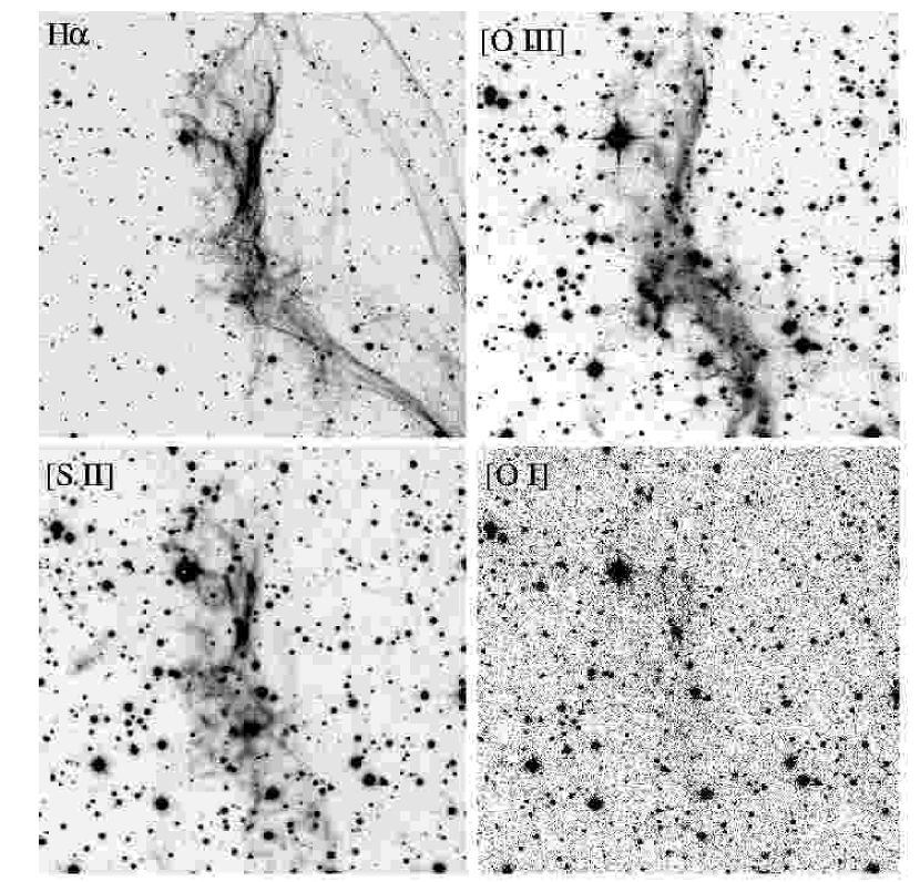
Figure 5: Images of the southwest cloud in H$\alpha$, [O III], [S II], and [O I]. Each panel covers a region of $7.7^{\prime}\times 7.7^{\prime}$. North is up and east is to the left.

The cloud’s optical appearance is considerably different when viewed in other emission lines. Figure 5 compares the cloud as seen in H$\alpha$, [O III], [S II] and [O I]. Whereas, the H$\alpha$ image shows a fairly sharp and filamentary appearance, the [O III] image is largely diffuse, while that of [S II] shows a more clumpy structure embedded in a diffuse component. Although the [O I] $\lambda$6300 emission is quite weak, its structure does not appear to closely resemble that of the other three line emission images.

Interestingly, the cloud’s [O III] and [S II] morphologies are substantially different to those seen in most other regions of the Cygnus Loop for these emission lines (Fesen, Blair, & Kirshner, 1982; Hester, Raymond, & Blair, 1994). Compared to most bright filamentary regions of the Cygnus Loop, which exhibit sharp and bright [O III] filaments, the southwest cloud’s [O III] structure is strikingly diffuse having few readily identifiable filaments. In addition, while H$\alpha$ and [S II] images are similar looking for most other regions in the remnant, that does not hold true here. The cloud’s appearance in [S II] is quite clumpy, with a few bright knots present, particularly in the cloud’s north and south ends. Also, the location of the peak [S II] and H$\alpha$ emissions in the cloud do not coincide. The same situation appears to be true for [O III] as well. Finally, the [O I] image shows little correlation to the [S II] image which might be expected in the presence of dense and lower ionization clumps.

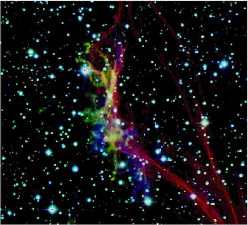
Figure 6: False color composite image of the southwest cloud. H$\alpha$ is in red, [O III] in blue, and [S II] in green.

To better visualize the cloud’s spatial emission differences, the H$\alpha$, [O III] and [S II] images were combined into a false color composite image (Fig. 6). In this composite image, Balmer-dominated filaments appear red, strong [O III] filaments appear blue, and strong [S II] regions are shown as green. Regions with strong H$\alpha$ and [S II] emission show up yellow, while regions strong in H$\alpha$ and [O III] appear magenta. Regions bright in [O III] and [S II] would look cyan, but this color is noticeably absent. Along the southern periphery, and to a lesser extent the northern periphery, H$\alpha$ emission is often seen immediately alongside strong [O III] emission. The eastern edges of the cloud are brightest in [S II] emission where, in comparison, the H$\alpha$ is relatively faint.

3.2 Optical Spectrophotometry

To quantify comparisons of the line emission strengths in [O III], [S II], and H$\alpha$, several apertures of various length ($\sim$ 5″– 20″) with a fixed 1.5″  width were extracted from the flux-calibrated images. The slices were made across the three main types of emission filaments present: suspected Balmer-dominated filaments, radiative shocks, and areas with unusually strong [S II] and [O III].

3.2.1 Balmer-Dominated Filaments

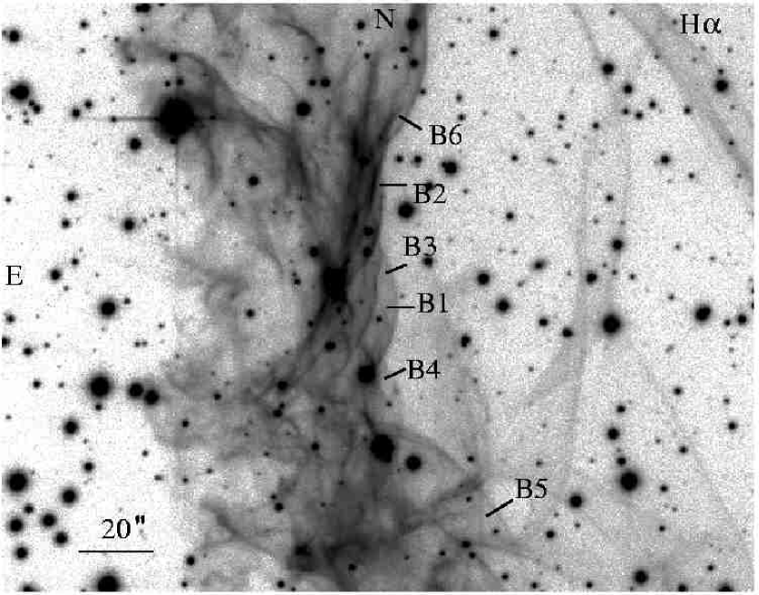
Figure 7: MDM 2.4 m H$\alpha$ image of the southwest cloud. Labels B1–B6 mark the location of several Balmer-dominated filaments discussed in the text.

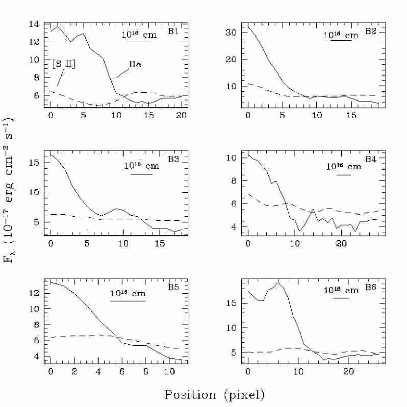
Figure 8: One-dimensional profiles for Balmer-dominated shock front regions B1 – B6 labeled in Figure 7. Plots show line strength of H$\alpha$ (solid line) versus [S II] $\lambda\lambda$6716,6731 (dashed line). Measured fluxes are per 1.5″ $\times$ 0.5″  pixels.

As already noted above in reference to Figure 4, numerous small scale shocks are present along the western edge of the cloud. For several of these suspected Balmer-dominated shocks, one-dimensional line flux profiles, measured normal to the shock front, were extracted from the H$\alpha$ and [S II] images. The positions of these aperture extractions are shown in Figure 7 and are labeled B1 – B6. The resulting 1D cuts across the six regions are shown in Fig. 8. The locations of our two long-slit spectra coincide with Positions B1 and B2. In all six regions, H$\alpha$ emission is seen to increase relative to [S II]. The relative increase occurs over a spatial scale of a few times 10¹⁶ cm. Given that these data have been background subtracted, the observed variations in the H$\alpha$/[S II] intensity ratio represent real, relative flux variations in the H$\alpha$ to [S II] ratio. The [S II] emission appears relatively constant from panel to panel, consistent with a diffuse, background. Furthermore, the relative increase between H$\alpha$ and [S II] is consistent from panel to panel, including the two spectroscopic Positions B1 and B2, suggesting that the ratios seen for Positions B3–B6 are real and not an artifact of our background subtraction technique.

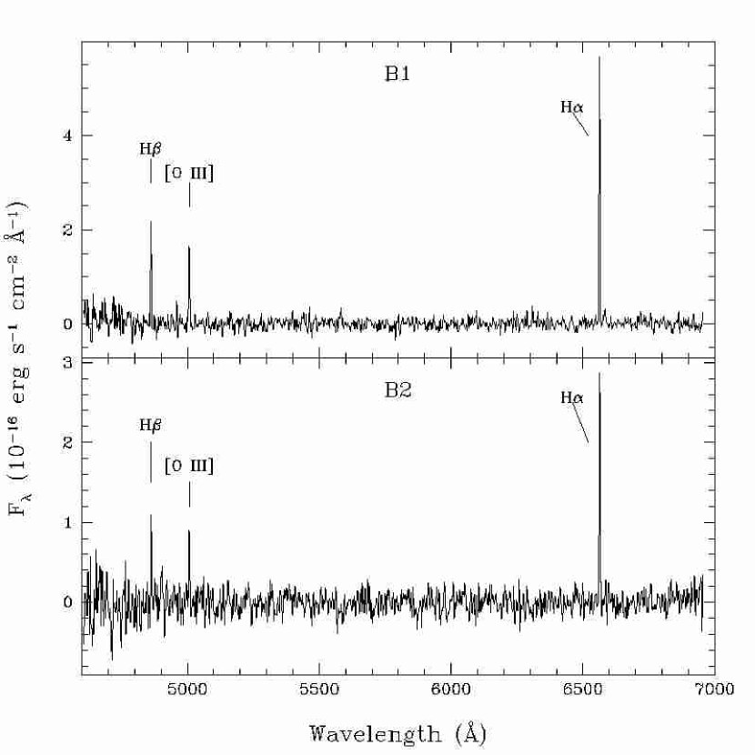
Figure 9: Emission line spectra for Positions B1 and B2.

The long-slit spectra for Positions B1 and B2 (Fig. 9) show bright Balmer emission, weak [O III] emission, and no detectable [S II] emission. The ratios of H$\alpha$/[O III] for regions B1 and B2 are 3.2 and 4.3 respectively (see Table 1). These spectra are very similar to spectra found in other regions of the Cygnus Loop located at or close to the shock front (Fesen, Blair, & Kirshner, 1982). This similarity adds credence to the belief that the small shock fronts along the western edge of the cloud are Balmer-dominated filaments.

3.2.2 [O III]-Bright Regions

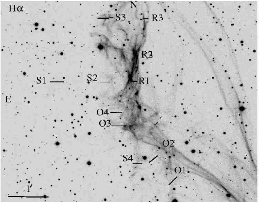
Figure 10: MDM 1.3 m H$\alpha$ image of the southwest cloud with radiative, [O III] bright, and [S II] bright regions marked where 1D line profiles were extracted.

In several portions of the Cygnus Loop’s brighter nebulosity, strong [O III] emission has been seen adjacent to Balmer-dominated emission. This has generally been interpreted as due to incomplete shocks (Blair et al., 1991). Incomplete shocks are often identified optically by [O III]/H$\alpha$ ratios $\geq$ 3. In order to investigate whether incomplete shocks could explain the strong [O III] emission along certain western portion of the southwest cloud, 1D line flux profiles were extracted for several regions, marked O1 – O4 in Figure 10, from the [O III] and H$\alpha$ images.

The four regions selected all lie along the cloud’s southern boundary where [O III] emission is especially prominent (see color image, Fig. 6). For all four regions we measured an [O III]/H$\alpha$ ratio of $2-3$. However, we suspect all four regions had background H$\alpha$ contamination from either Balmer-dominated filaments along the cloud southern edge or projected diffuse, pre-shock gas. We estimate that this contamination could account for nearly half of the measured H$\alpha$ intensity. This would increase the observed [O III]/H$\alpha$ ratio over 3, thereby indicating the presence of incomplete shocks. While this is likely to be true of the strong [O III] regions O1 and O2, Positions O3 and O4 lie well behind the shock front making their [O III] line emission nature less certain (see Section 4.2.2).

3.2.3 Radiative filaments

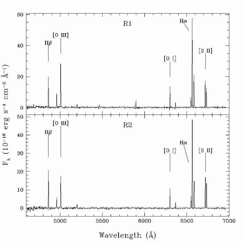
Figure 11: Emission line spectra for slit Positions R1 and R2.

Bright [S II], [O III], and H$\alpha$ emission regions are seen to lie east (downstream) of the Balmer-dominated filaments discussed above. Two regions, R1 and R2, extracted from our longslit spectra, are located near the center (R1) and to the north (R2) of the cloud (Fig. 10), several arcseconds behind the Balmer-dominated filaments. At R1 we see bright H$\alpha$, [S II], [O I], [O III] and H$\beta$, as shown in Figure 11. Line fluxes for the most prominent lines are listed in Table 1. At this position, we measured the electron-density-sensitive ratio [S II] 6717/6731 $=$ 1.4$\pm$0.1, which implies an electron density of 10 – 100 cm^-3 at T = 10⁴ K. Region R2 (Fig. 11) is located $\sim$ 45^′′ north of R1 and just a few arcseconds east of Balmer-dominated Position B2. Here the ratio [S II] 6717/6731 was again measured at 1.4 $\pm$ 0.1.

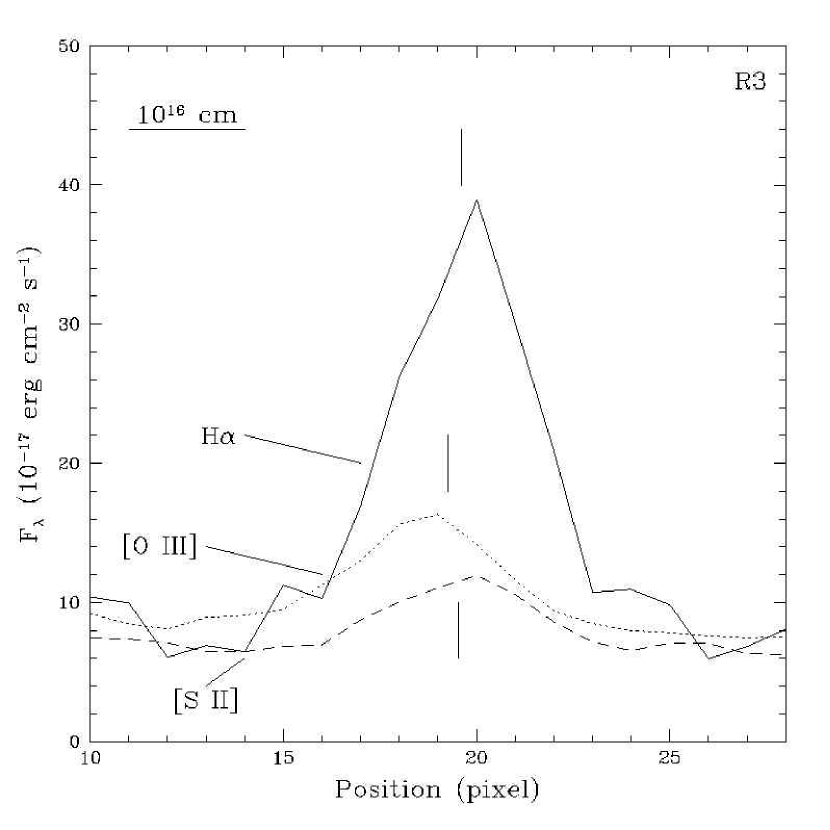
Figure 12: One dimensional emission profile for the bright radiative filament Position R3. Measured fluxes are per 1.5″ $\times$ 0.5″  pixels.

In addition to these 2D aperture spectra, we also extracted 1D emission profiles in H$\alpha$, [S II], and [O III] at Position R3, which is farther to the north (see Fig. 12). The line intensity plot (Fig. 12) shows maximum H$\alpha$ emission displaced some $<5\times 10^{15}$ cm ($\sim$ 2″) ahead of the [S II] peak intensity and $\sim$ 10¹⁶ cm ahead of the [O III] emission peak.

3.2.4 Sulfur-Bright Regions

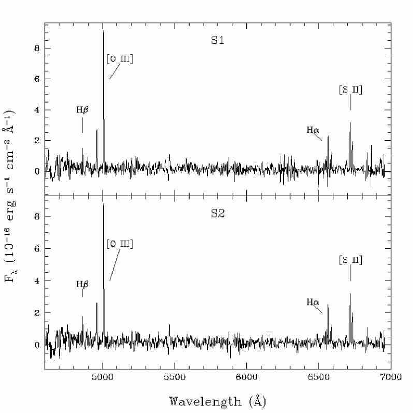
Figure 13: Emission line spectra for the [S II] bright slit positions S1 and S2.

There are several regions along the cloud’s eastern edge which exhibit especially strong [S II] emission. These can be seen as greenish clumps and filaments in Figure 6. Our central long-slit position crossed over two of these regions which we have labeled S1 and S2 in Figure 10. Spectra extracted for these two regions are shown in Figure 13. Although the spectra are fairly noisy, they clearly show [S II]/H$\alpha$ line ratios of $2-3$. This is much larger than the radiative filaments R1 and R2 values of 0.53 and 0.59, and are unusual compared to other regions in the Cygnus Loop (Fesen, Blair, & Kirshner, 1982). The density-sensitive ratio in these two regions is $\approx$ 1.35, implying n_e ${}_{>}\atop{}^{\sim}$ 100 cm^-3 at T = 10⁴ K), implying regions of somewhat higher density than those found in the radiative regions R1 and R2. These anomalously high [S II]/H$\alpha$ knots can be interpreted as clouds of gas that were shocked relatively long ago and have recombined to the extent that the Balmer line emission from recombination has begun to drop. The details depend upon the ratio of density to the radiation field, but this interpretation is supported by their location well behind the main shock.

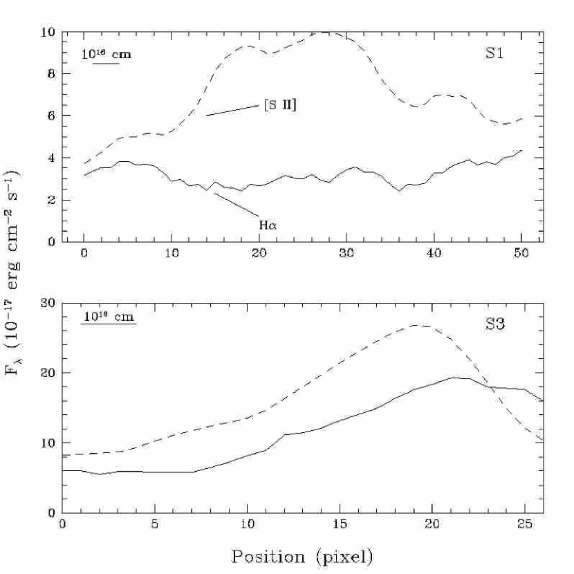
Figure 14: One-dimensional profiles for the [S II] bright regions S1 and S3. Measured fluxes are per 1.5″ $\times$ 0.5″  pixels.

In addition to the S1 and S2 spectra, we extracted 1D line profiles for two similarly greenish looking regions which we have labeled S3 and S4 on Figure 10. Both show smaller [S II]/H$\alpha$ ratios around 1.5. Furthermore, we find that these two regions differ from Regions S1 and S2 morphologically in that the [S II] emission peak is displaced eastward from the peak H$\alpha$ emission by a $\sim$ 3 $\times$ 10¹⁵ cm (see Fig. 14). Here we see that in Region S1, the H$\alpha$ emission is relatively constant compared to the [S II] emission, while in Region S3 we see that both the H$\alpha$ and [S II] emission ramp up with the [S II] emission reaching a maximum intensity $\sim$ 10¹⁶ cm behind the H$\alpha$.

3.3 X-ray Imaging Spectroscopy

As seen in Figure 1b, the global structure of the X-ray emitting gas in the Cygnus Loop closely resembles that of the optically-emitting gas. Furthermore, the X-ray morphology of the southwest cloud (Fig. 1 bottom right), appears very similar to the global morphology of the southwest cloud seen in H$\alpha$. In the X-ray, we see an undisturbed shock front both north and south of the cloud. This shock front is coincident with the Balmer-dominated shock front seen in the KPNO image. Also, the bright X-ray emission seen south of the cloud seems to correspond to the more tangled Balmer emission seen south of the cloud.

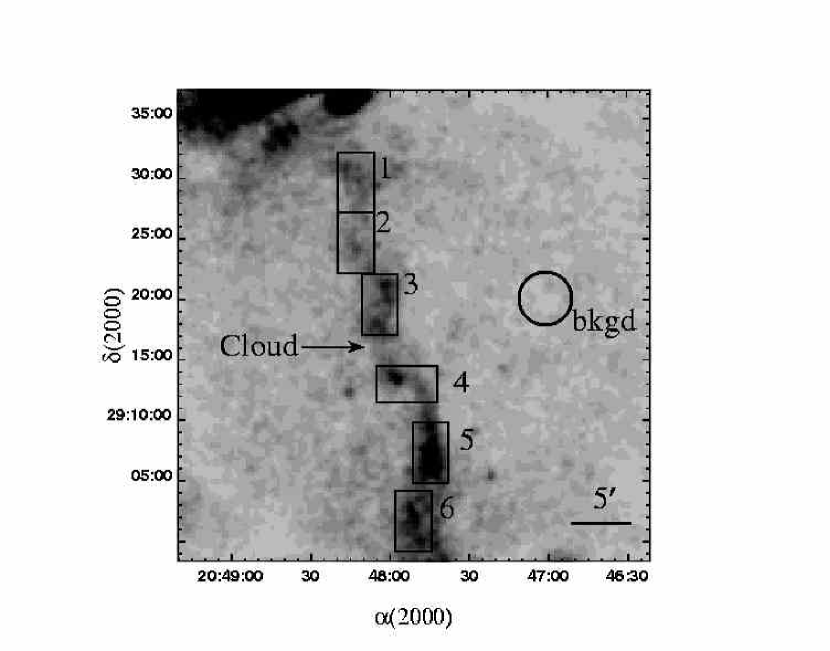
Figure 15: ROSAT PSPC image of the southwest cloud. The image has been smoothed to 1′  resolution.

Perhaps the most striking feature in the X-ray image is the absence of any appreciable emission from the cloud itself. In Figure 15, we have focused in on the cloud and surrounding shock front. There is bright X-ray emission, seen as spots, immediately north and south of the cloud, but the X-ray emission from the cloud itself is noticeably fainter than the surroundings. These bright X-ray spots are most likely due to enhanced emission as a result of a slight increase in density encountered by the X-ray emitting shock along the cloud’s outer boundaries. Much slower shocks ($\leq$ 150 km s^-1) would account for the lack of detectable X-ray emitting gas for the main body of the cloud.

We label in Figure 15 several regions around the southwest cloud where we extracted spectra for further analysis. The results of our fits are listed in Table 2. Regions 1 and 2 are associated with the undisturbed shock front north of the cloud. Here the shock is progressing rather uniformly through the ISM, which is apparent by the smoothness of the shock front, as well as uniformity in X-ray gas temperature ($\sim$ 0.13–0.12 keV). Region 3, immediately north of the cloud, has a lower temperature (0.11 $\pm$ 0.03 keV), but higher flux (F_x = 0.7 $\times$ 10^-12 erg cm^-2 s^-1) and emission measure (EM = 0.7 cm^-6 pc). A spatial examination of Region 3 reveals that the bulk of the X-ray emission arises from two knots within the 5′$\times$3′ box.

Region 4, immediately south of the cloud, is composed of the bright knot directly south of the cloud plus more diffuse X-ray emission trailing off to the west along the forward shock front. Here we again find the X-ray gas temperature to be $\sim$ 0.11 keV, which corresponds to a X-ray shock velocity of 290 km s^-1. However we find the X-ray flux and emission measure to be lower than in Region 3. Regions 5 and 6 are by far the brightest regions (10^-12 erg cm^-2 s^-1). As noted, these two regions are associated with bright Balmer emission seen south of the cloud in Figure 1. Here the shock front seems to be running into another ISM cloud, though the structure appears much more complicated than that of the southwest cloud.

In general, our results show hints of a systematic temperature gradient relative to the cloud. The X-ray emitting gas temperature drops at the clouds northern edge when approaching the cloud from the north (Regions 1, 2, & 3). This pattern is then reversed south of the cloud, with the temperature of Region 4 being essentially identical to that of Region 3, and then increasing towards Regions 5 and 6.

4 DISCUSSION

4.1 Dynamics

Shock-cloud interactions can be characterized by four stages of evolution (Klein, McKee, & Colella, 1994). The first stage occurs when the blast wave initially encounters the cloud, driving a strong shock into its face and forming a standing bow shock downstream. The second stage is cloud compression as the blast wave wraps around the rear of the cloud and re-converges upstream. A reflected shock forms at the re-converged shock front apex, which then travels back downstream into the cloud. This newly-formed shock, acting in concert with the slow internal cloud shocks traveling forward through the cloud, further compresses the cloud. The third stage involves a re-expansion of the cloud. This begins when the main cloud-shock reaches the downstream end of the cloud, causing a strong rarefaction to be driven back into the cloud, and leading to cloud re-expansion in the upstream direction. Finally, the cloud is destroyed as instabilities and differential forces due to the flow of intercloud gas past the cloud and cause it to fragment.

A useful parameter for measuring a shocked cloud’s evolution is what Klein et al. (1994) refer to as a “cloud crushing time”, t_cc. The cloud crushing time is the characteristic timescale for a cloud to be crushed by a shock moving through the cloud, and is therefore wholly dependent upon the cloud shock velocity ($t_{cc}=r_{c}/v_{s}$). However, the cloud shock velocity v_s is dependent upon the blast wave velocity v_b (Klein et al. 1994), so the cloud crushing time can be characterized by the blast wave velocity ($t_{cc}=\chi^{1/2}r_{c}/v_{b}$), where $\chi$ is the density contrast $\rho_{cloud}/\rho_{amb}$. In the case of the southwest cloud, we estimate t_cc to be $\approx$ 1500 yr assuming an initial cloud radius of $0.2$ pc (from optical measurements), a blast wave velocity of 290 km s^-1, and a density contrast, $\chi$, of 5 (Ku et al., 1984).

In their study, Klein et al. (1994) focused their analysis to clouds which are small compared to the blast wave. Small clouds are defined as those where the cloud crushing time $t_{cc}$ is of order the pressure variation time-scale $t_{P}$. The pressure variation time-scale for a dense cloud in a Sedov-Taylor blast wave is $t_{P}\simeq 0.1r_{c}/v_{b}$. Taking a blast wave velocity of 290 km s^-1 for the southwest cloud (see Section 3.3) and assuming that the cloud was initially roughly spherical ($r_{c}\simeq 0.2$ pc), then the pressure time-scale is $\sim$ 70 yr. Klein et al. (1994) define medium clouds as those with $t_{cc}{{}_{>}\atop{}^{\sim}}t_{P}$, so one can therefore view the southwest cloud in that context.

4.1.1 The Age of the Shock–Southwest Cloud Interaction

The structure of the southwest cloud itself and associated neighboring shock fronts suggest an early stage of shock-cloud interaction, probably somewhere in between stages one and two described above, with an age of $\sim$ 1200 yr. Several pieces of evidence support this.

First, Klein et al. (1994) argue that the wrap-around shocks will re-converge in a time of order 1.2 $t_{cc}$. Given the lack of a clear re-convergence point upstream of the southwest cloud, the cloud-shock interaction time must then be less than the time required for the wrap-around shocks to reconverge upstream of the cloud ($\approx$ 1800 yr). This conclusion is supported by the presence of numerous shock fronts inside the cloud lying at distances of up to 2′–3′ to the east (behind) the line of undisturbed H$\alpha$ shock front filaments. This shock structure is what would be expected at a relatively early shock–cloud interaction phase.

Secondly, shock–cloud models predict the formation of vortices along cloud edges as the shock passes by them. These vortices, and the resulting turbulence they create, are the result of Kelvin-Helmholtz (K-H) instabilities that form at the cloud-shock interface tangential to the shock normal. The formation of K-H instabilities occurs on a timescale comparable to the cloud crushing timescale. In Figure 3, several finger-like structures are seen to the north and south of the cloud. At first glance, these structures look like the result of K-H shearing. However, instabilities resulting from K-H shearing tend to follow the flow of the shock, whereas these fingers are flowing in the opposite sense. Therefore, our optical imaging of the southwest cloud shows no hint of K-H vortices along the edges of the cloud, thereby also suggesting an age less than $\sim$ 1500 yr.

Both age estimates above agree with a simple, crude age estimate of the cloud-shock interaction derived from assuming a roughly spherical cloud of radius 0.2 pc and shock velocity of 290 km s^-1. It would take $\sim$ 1500 yr for the shock to advance from front to the rear of the cloud, consistent with the location of the undisturbed shock front position as viewed in the H$\alpha$ images.

A final piece of evidence involves the lack of a clearly detectable standing bow shock in the postshock gas. Klein et al. (1994) state that a standing bow shock will form in a time $t_{b}=2r_{c}/v_{b}$. Using the above numbers as estimates, we find that the bow shock will form in 1300 yr. The lack of such a structure visible in the ROSAT X-ray image can be taken as evidence that this interaction is therefore much younger than a cloud crushing time, and at least as young as the $\sim$ 1300 yr bow shock formation timescale.

Therefore, given the assumed size of the cloud and shock velocity as measured from the X-ray observations, we suggest that the age of this cloud–shock interaction is $\approx$ 1200 yr. We estimate an uncertainty of $\pm$ 500 yr based upon the fact that we do not know the initial size of the cloud, and the fact that the shock velocity is an estimate based on the postshock gas temperature.

4.1.2 Cloud Shock Structures

As seen in Figures 3 and 4, the cloud contains a rich variety of shock structure on several scale lengths. As predicted by Klein et al. (1994), the main blast-wave wraps around the cloud with a curvature of order one cloud diameter. Of particular interest is the presence of several smaller shocks seen within the cloud itself. Intracloud shocks permeate the cloud on various scales, and at various angles to the main shock direction. This is suggestive of shock wave diffraction, analogous to a water wave passing through a narrow channel and exiting on the other side with curvature affected by the channel width. Similar arguments can be made with respect to the southwest cloud.

Initially, the cloud might have consisted of a low density intracloud medium permeated by small scale density variations (clumps). As the main shock wave progresses through the cloud, it is slowed by these density enhancements, while the intracloud shock travels in between them. These density enhancements go through the same cloud-shock interactions, only on a much smaller scale. In some cases the shock might stall, given that it is already traveling at a much slower velocity. However, the undisturbed shock will continue to carry momentum and energy through the less dense regions in the cloud, resulting in shocks with curvatures of order the clump separation.

The shock fronts within the cloud are about 7″ –10″ long. If the shock ends are “attached” to small regions of higher density, then the average distance between higher density clumps in the cloud is ${}_{<}\atop{}^{\sim}$10″. Assuming that the cloud was initially spherical with an angular size of $\sim$ 3′, we estimate that density fluctuations within this ISM cloud make up as much as $\sim$ 20% of the volume of the cloud. Furthermore, in order for this type of shock diffraction to occur, the density fluctuations must be at least of order of the density contrast between the cloud and the ISM.

Models for shock-cloud interactions often use a homogeneous initial density with a well defined boundary between the cloud and the intercloud zones. However, both our optical and X-ray observations show clearly that this is not the case for the southwest cloud. Decreased densities along a cloud’s outermost portions should result in a lower postshock density, and therefore a larger postshock cooling zone. This situation is actually seen along the cloud’s southern edge, where there is a large band of diffuse [O III] emission. Similarly, but less dramatically, the same appears to be occurring in the north.

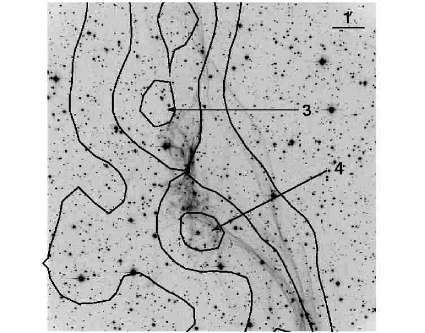
Figure 16: H$\alpha$ image of the southwest cloud overlaid with ROSAT PSPC X-ray contours. Contour intervals shown are 10.7, 12.8, and 14.9 counts. Regions 3 and 4 correspond to two bright X-ray knots visible in Figure 1 and tabulated in Table 2.

We find support for a gradual drop in density by noting that the X-ray emission is brightest along the north and south of the cloud, and centered somewhat east of the main shock front, as marked by Balmer-dominated filaments, that has already passed the cloud (see Fig. 16). If the edges of the cloud are of a lower density than the cloud itself, then the shock will not be slowed as much in its passage through this area. The comparison of the X-ray contours to the H$\alpha$ emission show little evidence for optical line emission near the X-ray knots, and this is confirmed by the lack of emission in [O III] and [S II].

4.1.3 Comparisons to the Southeast Cloud

Compared to the Cygnus Loop’s southeast cloud (Fesen, Kwitter, & Downes, 1992; Graham et al., 1995; Levenson & Graham, 2001), the southwest cloud appears to be in a much younger stage of shock-cloud interaction. The southeast cloud was initially identified as a small cloud in the late stage of shock-cloud interaction (Fesen, Kwitter, & Downes, 1992). Indeed, the resemblance to late-stage numerical models of shock-cloud interactions is striking (Bedogni & Woodward, 1990; Stone & Norman, 1992). However, more recent X-ray and optical studies (Graham et al., 1995; Levenson & Graham, 2001) suggest that the shock wave is interacting with the tip of a much larger cloud. Either way, however, the southwest and southeast clouds exhibit several similarities. Balmer-dominated filaments are seen to trace out the shock fronts as they wrap around and attempt to engulf both clouds. In the southwest cloud, X-ray hotspots are evident north and south of the cloud, while in the southeast cloud there is a similar hotspot along the southern edge of the cloud. Such hotspots seem to occur where the undisturbed shock front connects to the engulfing shock front. Finally, radiative filaments are seen to trail behind the Balmer-dominated filaments for both clouds.

However, there are also several distinct features of the southwest cloud which set it apart from the southeast cloud due to its youthful shock-cloud interaction. In the southeast cloud, there is bright X-ray emission associated with the shock as it wraps around the cloud. In contrast, we find virtually no X-ray emission associated with the main part of the southwest cloud. Also, in the southeast cloud a reverse shock is seen in the X-ray (Graham et al., 1995). No such reverse shock appears to exist in the southwest cloud. Given that a reverse shock will form shortly after the shock hits the cloud, the lack of a reverse shock suggests that it has not had time to form. A standing bow shock will only be seen if there is enough swept up material. The southwest cloud may be of a low enough density so that a standing X-ray bow shock will not form since the swept up gas density will never be above the critical density required for efficient heating and subsequent cooling.

4.2 Radiative Properties

4.2.1 Optical

In H$\alpha$ images, we see undisturbed Balmer-dominated filaments tracing out the shock front north and south of the cloud. Such filaments also mark where the shock front has progressed around the back side of the cloud. We also see Balmer-dominated emission coming from several small shocks inside the cloud.

The cloud’s optical appearance changes radically when viewed in line emissions from conventional radiative-type emission regions. While the H $\alpha$ emission is characterized by thin, bright filamentary structure, just the opposite is true for its [O III] emission. As shown in Figure 5, the [O III] emission is largely diffuse, with just a few sharp filaments. In addition, there is the relative lack of [O III] emission north of the cloud compared to the south. A similar asymmetry is also seen in H$\alpha$ which might imply a density gradient along the north-south axis of the cloud. In contrast to both the [O III] and H$\alpha$ emission morphologies, the cloud’s strong [S II] emission structure is limited to a few sharp filaments and some faint, diffuse emission patches (Fig. 5).

Compared to the remnant’s bright radiative northwestern and northeastern limb filaments (e.g. Hester (1987)), the southwest cloud shows both similarities and differences when the H$\alpha$, [S II], and [O III] emissions are viewed together (Fig. 6). The cloud’s northern extremity shows postshock line emission stratification like that discussed by (Hester, 1987). That is, Balmer-dominated filaments are followed closely by a region strong in [O III] emission followed in turn by strong [S II] line emissions (Fig. 12). Also, in the eastern part of this northern section, one finds bright, well defined [S II] filaments, some diffuse H$\alpha$ emission but no corresponding [O III] emission, suggesting postshock cooling regions farther downstream ($\sim$ 10¹⁷ cm) from the shock front.

In general, one finds Balmer-dominated filaments that may or may not be followed by [S II] or [O III] radiative emission. This is consistent with a resolved postshock cooling zone where first strong [O III] line emission is seen followed by [S II] and H$\alpha$. In the possibly older, denser shocked cloud regions only [S II] emission remains. The lower density regions of the cloud will have longer postshock cooling times which may account for the diffuse nature of the cloud’s [O III] emission structure. The lack of clear line stratifications in the cloud’s southern half may be an indication of a generally lower density compared to the north. This, in turn, would have led to the presence of numerous small scale shock structures like that seen in H$\alpha$.

Region S1 is positioned well behind ($\sim$ 1′) the advancing shock front. As shown in Figure 13 and Figure 14, there is little Balmer emission, but bright emission from forbidden lines. The lack of Balmer emission, coupled with the strong emission in [S II] and [O III] suggest that this is a region of strong radiative cooling. Furthermore, in Figure 6, we find that the sulfur-bright regions are more compact than the diffuse oxygen-bright regions. This is consistent with our assumption that the [S II] emission is arising from regions of cooler, higher density gas, which might be enveloped in a warmer [O III] bright shell.

In conclusion, while the cloud’s overall shock structure is not unlike that expected for a recently shocked cloud, the structure and complexity of the line emission features was somewhat unexpected. Like elsewhere in the Cygnus Loop, sharp Balmer-dominated filaments nicely trace out the shock front. But the emission structure seen in other emission bands differs sharply from that seen in other regions of the remnant (Levenson, et al., 1998). This is especially true in terms of the largely diffuse [O III] emission and the clumpy far-downstream [S II] emission structure. Such emission features set this cloud’s emission properties apart from the those seen before in the well-studied, dense cloud regions of the Cygnus Loop.

4.2.2 X-ray Morphology and Radiative Shock Models

The X-ray morphology generally matches that seen in H$\alpha$. That is, one sees the X-ray emission trace the Balmer emission north to south (see Fig. 1). In addition, the bright H$\alpha$ filaments south of the cloud correlate well with the extended X-ray emission located several arcminutes south of the cloud (Regions 5 and 6 of Fig. 15). This region itself may be another shock-cloud interaction, due to the clumpy appearance of the optical emission here. Regions 3 and 4 correspond to the north and south edges of the cloud, where there is a brightening in the observed X-ray emission.

The fact that the X-ray emission arises along the edges of the cloud and not from the interior of the cloud is puzzling. One possibility is that there is a density gradient within the cloud. The lower-density component of the cloud edges would not slow the shock below X-ray emitting temperatures, while the higher-density core of the cloud would slow the shock. The existence of X-rays along the edges of the cloud is in sharp contrast to other regions of the SNR, where the bulk of the X-ray emission arises from shocks reflected off of ISM clouds.

The X-ray spectral fits for Regions 3 and 4 give electron densities of $1.1$ and $0.7$ cm^-3 (assuming a line-of-sight depth of 0.6 pc) and temperatures of 1.2 $\times$ 10⁶ K. For complete electron-ion equilibration at this temperature, the shock velocities are $\sim$ 290 km s^-1. Therefore, for the X-rays, the ram pressure is $\sim$ 1.2 $\times$ 10^-9 dyne cm^-2, which is consistent with both the X-ray emitting gas found in the XA region ($\sim$ 9 $\times$ 10^-9 dyne cm^-2; Levenson & Graham 2001) and the southeast cloud ($\sim$ 10^-9 dyne cm^-2; Graham et al. 1995). It is worth noting that the shock velocity derived from X-ray measurements is $\sim$ 100 km s^-1 lower than what is found elsewhere in the remnant. However, the blowout region of the remnant may be evolving differently than the main SNR shell, so it is not surprising that the shock velocity here is different than elsewhere.

Our plots show several examples where the [O III] seems to follow the H$\alpha$ by about 1″  (e.g., Fig. 12). If the separation corresponds to the distance between the shock (going into partially neutral gas) and the peak of the [O III] emissivity, then the shock velocity v_s must be more than 120 km s^-1. Models were run with a preshock neutral fraction of 0.5. The preshock neutral fraction cannot be larger than about 0.7 because the shock produced enough ionizing photons even when it is nonradiative to ionize 30% of the H. On the other hand, the ionized fraction of H cannot be less than 0.3 without making the initial H$\alpha$ too weak compared with the [O III] peak. A shock speed of 120 km s^-1 is too slow for this neutral fraction as might be expected from the lower effective shock speed with partially neutral preshock gas (Cox & Raymond, 1985). An effective shock speed of 106 km s^-1 will not completely ionize the gas beyond [O III] so there is no separate peak in emissivity behind the shock.

We also computed the H$\alpha$ brightness assuming that the slit crosses a 1.5″  high section of shock with a depth along the line-of-sight l = 5′  = 0.63 pc (the size of our extraction regions in the X-ray analysis, and the extent of the filaments in the plane of the sky). We list the results from these models in Table 3 for a distance of 440 pc, with the H$\alpha$–[O III] separation designated as $\Delta$, the pre-shock number density expected from equal ram pressure with the X-ray gas as n_cloud, and the H$\alpha$ brightness, assuming a preshock neutral fraction of 0.5, as I_Hα.

From the values of $\Delta$ in Table 3, V_shock must be less than about 160 km s^-1 and the post-shock number density, n_PS, must be about 3, implying that the ram pressure for the cloud shock is slightly higher than that for the X-ray shock. Considering that the X-ray gas is off to the sides of the optical cloud, this seems plausible. From I_Hα, one concludes that the line of sight distance $l$ to produce the $\sim$ 1.5 $\times$ 10^-15 erg cm^-2 s^-1 with n_PS $\sim$ 3 must be smaller than the X-ray depth, not surprising given that this is a small filament, l_Hα $<$ l_X = 4 $\times$ 10¹⁷ cm.

Overall, our results are self-consistent within the constraints of connecting optical and X-ray observations and the limits of the models. One expects that shocks faster than 150 km s^-1 would be thermally unstable (Innes, 1992) so the higher velocity models listed in Table 3 are not entirely reliable. But to first order, the cooling length of the gas should be approximately correct with the H$\alpha$ brightness given by the product of preshock neutral fraction and shock speed. The line of sight depth assumed for the X-ray emission also seems reasonable within the limitations of time-dependent ionization and depletion of refractory elements on grains. Both these effects these tend to decrease the emissivity, implying a density a little higher (no more than a factor of 2) than the numbers we derive.

5 CONCLUSIONS

ROSAT X-ray data and ground based optical data for the southwestern region of the Cygnus Loop SNR show the early stages of the interaction of a blast wave with a cloud in unprecedented detail. From our study of this shocked cloud, we conclude the following:

1) The cloud began interacting with the shock $\sim 1200$ yr ago. This is supported by the lack of a standing bow shock behind the cloud, the lack of a shock reconvergence point west of the cloud, and no evidence for instability formation along the edges of the cloud.

2) The optical morphology of the cloud is substantially different than what is seen in the brighter regions of the remnant. Whereas many of the brighter regions of the Cygnus Loop are the result of $\sim$ 400 km s^-1 shocks hitting relatively higher density material, the low density and low shock velocity nature of this region stretches the postshock cooling zone resulting in the diffuse [O III] and clumpy [S II] emissions observed.

3) The cloud’s X-ray emission structure is also unlike that seen in the brighter optical and X-ray regions of the remnant. Little or no X-ray emission is associated with the cloud itself, but there is bright X-ray emission associated with the northern and southern peripheries of the cloud. Furthermore, we derive a shock velocity of 290 km s^-1 which is significantly lower than shock velocities found in other parts of the Cygnus Loop remnant.

4) Small scale density fluctuations were found to exist within this ISM cloud which significantly altered the progression of the shock through the cloud. This is seen by the presence of multiple small scale shocks which are seen throughout the cloud.

In summary, this relatively isolated, low density cloud in the southwest limb of the Cygnus Loop has provided a revealing snapshot of the very early stages of a shock-cloud interaction. It shows how a cloud’s initial density structure can strongly influence the observed optical and kinematic morphology of the postshock gas. Further analyses of some of the exquisite details of this shock-cloud interaction may provide additional diagnostics with regards to two- and three-dimensional models of shocks overrunning ISM clouds.

Table 1: Measured Line Fluxes (H$\beta$ = 100)

Line	$\lambda$				Fλ
	(Å)	R1	R2	S1	S2	B1	B2
H$\beta$	4861	100	100	$\cdots$	$\cdots$	$\cdots$	100
$[{\rm O\,III}]$	4959	56	27	470	260	$\cdots$	$\cdots$
$[{\rm O\,III}]$	5007	150	98	1350	780	93	80
$[{\rm O\,I}]$	6301	71	62	$\cdots$	$\cdots$	$\cdots$	$\cdots$
$[{\rm O\,I}]$	6365	19	22	$\cdots$	$\cdots$	$\cdots$	$\cdots$
$[{\rm N\,II}]$	6549	35	32	$\cdots$	$\cdots$	$\cdots$	$\cdots$
H$\alpha$	6563	338	317	300	300	300	340
$[{\rm N\,II}]$	6584	104	100	$\cdots$	$\cdots$	$\cdots$	$\cdots$
$[{\rm S\,II}]$	6717	104	110	495	320	$\cdots$	$\cdots$
$[{\rm S\,II}]$	6731	75	78	360	240	$\cdots$	$\cdots$
F(H$\beta$)		8.0	7.9	$\cdots$	$\cdots$	$\cdots$	0.4
F(H$\alpha$)		$\cdots$	$\cdots$	0.9	1.5	2.6	$\cdots$

Table 2: Model to the X-ray spectra of the southwest cloud and vicinity

Region	$\alpha$ (J2000)	$\delta$ (J2000)	kT	NH	Fx	EM	$\chi^{2}$ (d.o.f)
	h  m  s.s	°   ′   ″	(keV)	1020 atoms cm-3	(0.1–1.0 keV)	cm-6 pc
1	20 48 13.2	29 29 42	0.13${}^{+0.01}_{-0.04}$	1.6${}^{+2.8}_{-0.7}$	0.5	0.45	12.5 (11)
2	20 48 13.2	29 24 42	0.12${}^{+0.06}_{-0.03}$	3.1${}^{+5.5}_{-1.6}$	0.5	0.32	8.91 (6)
3	20 48 04.0	29 19 37	0.11${}^{+0.03}_{-0.03}$	2.8${}^{+0.4}_{-0.4}$	0.7	0.60	10.3 (6)
4	20 47 52.1	29 13 07	0.11${}^{+0.05}_{-0.04}$	1.6${}^{+0.4}_{-0.3}$	0.4	0.45	7.06 (5)
5	20 47 46.4	29 08 07	0.13${}^{+0.05}_{-0.04}$	1.6${}^{+0.4}_{-0.5}$	1.0	0.99	6.02 (5)
6	20 47 46.4	29 02 45	0.14${}^{+0.02}_{-0.04}$	1.6${}^{+0.8}_{-0.6}$	1.0	0.74	20.2 (11)

Table 3: Model fits to the radiative shocks seen in the southwest Cloud

Vshock	$\Delta$	ncloud	IHα	Popt / PX-ray
km s-1	″/ nPS	cm-3	10-15 erg s-1 cm-2 $\times$ nPS
140	4	1.0	3.5	0.75
150	5	0.87	3.8	0.86
160	8	0.76	4.0	0.97
170	11	0.68	4.2	1.1
180	16	0.60	4.5	1.2
190	26	0.54	4.8	1.4
200	40	0.50	5.0	1.5

Figure 1: a (top): Digital Sky Survey H$\alpha$ image of the Cygnus Loop showing the location of the southwest cloud. (bottom): KPNO Schmidt image of the southwest cloud. b (top): ROSAT PSPC mosaic of the Cygnus Loop in the 0.2 – 2.4 keV band. (bottom): ROSAT PSPC image of the southwest region of the Cygnus Loop. Both images have been logarithmically scaled.

Figure 2: KPNO Schmidt H$\alpha$ image of the southwest cloud and vicinity. North is up and east is to the left.

Figure 3: MDM 1.3 m H$\alpha$ image of the southwest cloud region. Image as shown covers a $11^{\prime}\times 11^{\prime}$ FOV. North is up and east is to the left.

Figure 4: MDM 2.4 m H$\alpha$ image of the southwest cloud. Arrows mark the positions of several small shock fronts inside the cloud. Image as shown covers a $3.5^{\prime}\times 2.7^{\prime}$ FOV. North is up and east is to the left. The image has been scaled logarithmically to show the internal shocks.

References

- Arnaud & Dorman (2000) Arnaud, K. & Dorman, B. 2000, Xspec (Greenbelt: NASA/GSFC), p. 113
- Bedogni & Woodward (1990) Bedogni, R. & Woodward, P. R. 1990, A&A, 231, 481
- Blair et al. (1991) Blair, W. P. et al. 1991, ApJ, 379, L33
- Blair et al. (1999) Blair, W. P., Sankrit, R., Raymond, J. C., & Long, K. S. 1999, AJ, 118, 942
- Bocchino, Maggio, & Sciortino (1994) Bocchino, F., Maggio, A., & Sciortino, S. 1994, ApJ, 437, 209
- Charles, Kahn, & McKee (1985) Charles, P. A., Kahn, S. M., & McKee, C. F. 1985, ApJ, 295, 456
- Chevalier & Raymond (1978) Chevalier, R. A. & Raymond, J. C. 1978, ApJ, 225, L27
- Chevalier, Raymond, & Kirshner (1980) Chevalier, R. A., Raymond, J. C., & Kirshner, R. P. 1980, ApJ, 235, 186
- Churazov et al. (1996) Churazov, E., Gilfanov, M., Forman, W., & Jones, C. 1996, ApJ, 471, 673.
- Cox (1972) Cox, D. P. 1972, ApJ, 178, 143
- Cox & Raymond (1985) Cox, D. P. & Raymond, J. C. 1985, ApJ, 298, 651
- Danforth et al. (2000) Danforth, C. W., Cornett, R. H., Levenson, N. A., Blair, W. P., & Stecher, T. P. 2000, AJ, 119, 2319
- DeNoyer (1975) DeNoyer, L. K. 1975, ApJ, 196, 479
- Fesen, Blair, & Kirshner (1982) Fesen, R. A., Blair, W. P., & Kirshner, R. P. 1982, ApJ, 262, 171
- Fesen, Blair, & Kirshner (1985) Fesen, R. A., Blair, W. P., & Kirshner, R. P. 1985, ApJ, 292, 29
- Fesen, Kwitter, & Downes (1992) Fesen, R. A., Kwitter, K. B., & Downes, R. A. 1992, AJ, 104, 719
- Graham et al. (1995) Graham, J. R., Levenson, N. A., Hester, J. J., Raymond, J. C., & Petre, R. 1995, ApJ, 444, 787
- Heathcote & Brand (1983) Heathcote, S. R. & Brand, P. W. J. L. 1983, MNRAS, 203, 67
- Hester, Danielson, & Raymond (1986a) Hester, J. J., Danielson, G. E., & Raymond, J. C. 1986, ApJ, 303, L17
- Hester & Cox (1986) Hester, J. J. & Cox, D. P. 1986, ApJ, 300, 675
- Hester (1987) Hester, J. J. 1987, ApJ, 314, 187
- Hester, Raymond, & Blair (1994) Hester, J. J., Raymond, J. C., & Blair, W. P. 1994, ApJ, 420, 721
- Innes (1992) Innes, D. E. 1992, A&A, 256, 660.
- Klein et al. (1991) Klein, R. I., McKee, C. F., & Collela, P. 1991, in Supernovae, edited by S. E. Woosley (Springer, New York), p. 696
- Klein, McKee, & Colella (1994) Klein, R. I., McKee, C. F., & Colella, P. 1994, ApJ, 420, 213
- Ku et al. (1984) Ku, W. H., Kahn, S. M., Pisarski, R., & Long, K. S. 1984, ApJ, 278, 615
- Levenson et al. (1996) Levenson, N. A., Graham, J. R., Hester, J. J., & Petre, R. 1996, ApJ, 468, 323
- Levenson, et al. (1998) Levenson, N. A., Graham, J. R., Keller, L. D., & Richter, M. J. 1998, ApJS, 118, 541
- Levenson, Graham, & Snowden (1999) Levenson, N. A., Graham, J. R., & Snowden, S. L. 1999, ApJ, 526, 874
- Levenson & Graham (2001) Levenson, N. A. & Graham, J. R. 2001, ApJ, 559, 948
- Long et al. (1992) Long, K. S., Blair, W. P., Vancura, O., Bowers, C. W., Davidsen, A. F., & Raymond, J. C. 1992, ApJ, 400, 214
- McCray & Snow (1979) McCray, R. & Snow, T. P. 1979, ARA&A, 17, 213
- McKee & Cowie (1975) McKee, C. F. & Cowie, L. L. 1975, ApJ, 195, 715
- Morrison & McCammon (1983) Morrison, R. & McCammon, D. 1983, ApJ, 270, 119
- Nousek & Lesser (1993) Nousek, J. A., & Lesser, A. 1993, ROSAT Newsletter, 8, 13
- Parker (1967) Parker, R. A. R. 1967, ApJ, 149, 363
- Raymond & Smith (1977) Raymond, J. C. & Smith, B. W. 1977, ApJS, 35, 419
- Raymond et al. (1980) Raymond, J. C., Hartmann, L., Black, J. H., Dupree, A. K., & Wolff, R. S. 1980, ApJ, 238, 881
- Raymond, Blair, Fesen, & Gull (1983) Raymond, J. C., Blair, W. P., Fesen, R. A., & Gull, T. R. 1983, ApJ, 275, 636
- Scoville et al. (1977) Scoville, N. Z., Irvine, W. M., Wannier, P. G., & Predmore, C. R. 1977, ApJ, 216, 320
- Snowden & Freyberg (1993) Snowden, S. L. & Freyberg, M. J. 1993, ApJ, 404, 403
- Snowden & Kuntz (1998) Snowden, S.L., & Kuntz, K.D. 1998, Cookbook for Analysis Procedures for ROSAT XRT/PSPC Observations of Extended Objects and the Diffuse Background, Part I: Individual Observations (Greenbelt: NASA/GSFC)
- Snowden et al. (1992) Snowden, S. L., Plucinsky, P. P., Briel, U., Hasinger, G., & Pfeffermann, E. 1992, ApJ, 393, 819
- Snowden et al. (1994) Snowden, S. L., McCammon, D., Burrows, D. N., & Mendenhall, J. A. 1994, ApJ, 424, 714
- Stone & Norman (1992) Stone, J. M. & Norman, M. L. 1992, ApJ, 390, L17
- Teske (1990) Teske, R. G. 1990, ApJ, 365, 256
- Trümper (1983) Trümper, J. 1983, Adv. Space Res, 4, 241
- Woodward (1976) Woodward, P. R. 1976, ApJ, 207, 484