Noise and the strong signal limit in radio astronomical measurement

Abstract

The random error of radioastronomical measurements is usually computed in the weak-signal limit, which assumes that the system temperature is sensibly the same on and off source, or with and without a spectral line. This assumption is often very poor. We give examples of common situations in which it is important to distinguish the system noise in signal-bearing and signal-free regions.

1 Introduction

Few experiments are performed without some attempt at estimating their errors, and the random errors of measurement in radio astronomy are typically determined in one general way. Some form of comparison is performed whereby samples are taken toward and away from a signal source, or with and without a spectral line. Subsequent analysis proceeds under the assumption that random errors everywhere in the dataset are as given by the statistical properties manifested in the signal-free regions. No attempt is made to measure the variances of signal-bearing and signal-free samples separately during the experiment, and, after the fact, random errors of measurement in signal-bearing samples are obscured because the form of the signal is arbitrary. Discussions of fitting and profile analysis invariably assume that measurement variances are the same with or without the signal, as for instance the Zeeman analysis of Marshall (1995) or the fitting of functions ($e.g.$ Gaussians) by Kaper et al. (1966) or Rieu (1969). Textbook discussions contain no suggestion that system noise is influenced by the presence of a signal or that samples with different variances may be interleaved in the same datastream (Kraus, 1986; Burke & Graham-Smith, 1997; Rohlfs et al., 2000).

Yet, such treatment has been flawed for a surprisingly long time. 100 K H I lines have been routinely observed with sub-100 K receiving systems for more than 30 years. Continuum sources whose antenna temperatures exceed the equivalent noise temperature of the receiving equipment have been observed even longer. The error of measurement in signal-bearing samples is often significantly different – with current receivers it could easily be a factor of 5 at the peak of a strong galactic H I emission line – but the difference has been ignored.

Error estimates determine confidence levels and even data containing strong signals can be compromised by misunderstanding of their significance; for instance, when two very strong signals are differenced to detect a smaller one in H I emission-absorption experiments and searches for Zeeman splitting. Considering how slowly experimental errors typically improve with the amount of time invested in an experiment, it follows that changes in the acknowledged errors of an experiment are equivalent to much larger differences in the observing time required to reach them. $A~{}priori$ knowledge of errors is an important element in the design of experiments and these considerations may have a significant effect on the planning of an observing session. They should be implemented in the software which supports analysis.

The purpose of this work is to illustrate a variety of common situations where random error is dominated by the presence of a signal. In the following section some basics of radio astronomy measurement are sketched. These are used to analyse the statistics of noise and the errors of component fitting when signals are present in emission and absorption. The final section is a brief summary with an even briefer mention of the extension of these notions to aperture synthesis.

2 Power, temperature and noise

2.1 Basics

A temperature scale is established whereby power is compared to the classical power spectral density kT (W Hz^-1) in a resistor in thermal equilibrium at temperature T (Dicke, 1946; Kraus, 1986; Rohlfs et al., 2000). The output power level of the telescope system is then quoted as a ‘system temperature’, $i.e.$, k${\rm T}_{\rm sys}$. The actual power density $h\nu/(e^{h\nu/kT}-1)+h\nu/2$ (Callen & Welton, 1951) reduces to kT only in the Rayleigh-Jeans limit and when zero-point fluctuations are ignored.

In our simplified discussion we assert ${\rm T}_{\rm sys}$ = ${\rm T}_{\rm T}$+ ${\rm T}_{\rm A}$. ${\rm T}_{\rm T}$ represents everything which does not depend on any particular source or input signal and we assume that it is a constant or constant function of frequency $\nu$: possible dependencies of ${\rm T}_{\rm T}$ are suppressed for convenience of notation. Observing at a frequency $\nu$ entails a minimum contribution of $h\nu/k$ to ${\rm T}_{\rm sys}$, which is included in ${\rm T}_{\rm T}$.

${\rm T}_{\rm A}$ represents a signal external to the telescope. The equivalent temperature of a signal is its ‘antenna temperature’ which by convention is related to the incident flux density S_ν (W m^-2 Hz^-1) as S_ν$=2$ k${\rm T}_{\rm A}$/A. The effective area A is proportional to the geometric area of the telescope aperture.

The signal may be confined in space or frequency, so we write ${\rm T}_{\rm A}$ = ${\rm T}_{\rm A}$(v) where v is some combination of independent variables. In the presence of signal the power density is k${\rm T}_{\rm sys}$(v) = k${\rm T}_{\rm T}$ + k${\rm T}_{\rm A}$(v) and the dependence of ${\rm T}_{\rm A}$ upon v makes ${\rm T}_{\rm sys}$ similarly dependent. If v represents the pointing of the telescope, added power comes and goes as the telescope moves. Alternatively, v may be velocity or frequency, and, as far as the receiver and square-law detector are concerned, the presence of signal at some v=v^′ is not manifested at v $<>$ v^′. The passband may be translated or inverted by mixing, but the receiver and detector electronics are entirely linear in frequency. The spectrum is not jumbled nor is it appreciably smoothed until it is integrated and channelized in the so-called ‘backend ’. In Sect. 2.7 we discuss an exception to this linearity, namely, quantization noise in digital correlator spectrometers.

2.2 Passband or system noise as a measurement variance

Eventually a datastream is formed from samples of ${\rm T}_{\rm sys}$, each of duration t (say) taken over a spectral width $\Delta\nu$; this could be a spectrum, a continuum drift scan, etc. Associated with measurement of the output power k${\rm T}_{\rm sys}$ there is a variance given by the Dicke (1946) or radiometer equation:

$$\Delta{\rm T(v)}^{2}={{\mbox{${\rm T}_{\rm sys}$}^{2}({\rm v})}\over{{\rm N}}}={({\mbox{${\rm T}_{\rm T}$}+\mbox{${\rm T}_{\rm A}$}({\rm v}))^{2}}\over{{\rm N}}}$$

The dimensionless quantity N $\equiv\Delta\nu{\rm t}$ is the product of the bandwidth measured in Hz and the integration time in seconds. Precise determination of the output power density kT within a band $\Delta\nu$ is done by averaging N independent samples. Within a band of width $\Delta\nu$ about some frequency $\nu$, the contained frequency components beat each other down to a frequency range 0..$\Delta\nu$ so that all appear together summed within one channel of this width.

Radiometer noise in the output datastream is the measurement variance of the power, independent of whether that power was contributed by ${\rm T}_{\rm T}$ or ${\rm T}_{\rm A}$. So the variance of the measured strength of an emission line, usually considered to be set only by ${\rm T}_{\rm T}$, actually increases in proportion to the source strength itself, weakly for weak signals and more strongly for very strong ones.

2.3 Normalization and noise in real-world experiments

As examples of the way that random error is affected by considerations of experimental design, we compare some common methods of data-taking. We consider that it is possible to take data “on”- or “off”-source; if the data are spectra, even the on-source data may have regions of the bandpass which are signal-free.

In the simplest case where data are taken while staring at the source, the variance is given directly by Eqn. 1

$$\Delta{\rm T(v)}^{2}~{}(on)~{}={({\mbox{${\rm T}_{\rm T}$}+\mbox{${\rm T}_{\rm A}$}({\rm v}))^{2}}\over{{\rm N_{on}}}}.$$

When on- and off-source data are differenced the rms is

$$\Delta{\rm T(v)}^{2}~{}(on-off)~{}={({\mbox{${\rm T}_{\rm T}$}+\mbox{${\rm T}_{\rm A}$}({\rm v}))^{2}}\over{{\rm N_{on}}}}+{{\mbox{${\rm T}_{\rm T}$}^{2}}\over{{\rm N_{off}}}}$$

and the rms in signal-free regions is increased relative to that at the signal peak.

In some cases a quotient is formed from on- and off-source data: the mean off-source power level is equated to a number, ${\rm T}_{\rm T}$, and data appear in the form ${\rm T}_{\rm T}$(on/off) or ${\rm T}_{\rm T}$(on-off)/off. Both have the variance

$$\Delta{\rm T(v)}^{2}~{}(on/off)~{}={({\mbox{${\rm T}_{\rm T}$}+\mbox{${\rm T}_{\rm A}$}({\rm v}))^{2}}\over{{\rm N_{on}}}}+{({\mbox{${\rm T}_{\rm T}$}+\mbox{${\rm T}_{\rm A}$}({\rm v}))^{2}}\over{{\rm N_{off}}}}$$

so formation of the quotient increases the rms in the signal-bearing regions relative to the case where simple differencing is done, and everwhere relative to the pure “on” spectrum.

Because of such considerations, it is not possible to calculate the random error in signal-bearing regions, even given the empirical rms in the signal-free regions and the system properties which pertain to them, unless it is also understood how the data were taken.

2.4 Emission line profiles

One obvious example of the strong signal limit of a spectral line is galactic atomic hydrogen. Fig. 1 shows a typical low latitude galactic H I profile observed with a 25m telescope (Hartmann & Burton, 1997) during the Leiden-Dwingeloo Sky Survey (LDSS). In the lower panel, the scale is expanded to show how the $\pm 1\sigma$ noise envelope varies for data taken in the form (on-off)/off with $\mbox{${\rm T}_{\rm T}$}=36$K, a typical value during the survey. The spectrum in Fig. 1 still has very high peak/rms signal-noise (465:1), but not nearly as good (1700:1) as implied by the 0.06 K rms over the baseline regions: the rms error of the integrated brightness is nearly twice as high as that estimated from the baseline rms level. H I is now commonly observed with $\mbox{${\rm T}_{\rm T}$}=15-25$K. If the same profile were reobserved with ${\rm T}_{\rm T}$ = 18 K for one-fourth the amount of time (to reach the same baseline rms ), the line-generated rms error would be twice as high again.

From the LDSS, we find that some 41% of the sky contains H I with a peak brightness $\mbox{${\rm T}_{\rm B}$}\geq 20$K, 33% has $\mbox{${\rm T}_{\rm B}$}\geq 30$K and 27% has $\mbox{${\rm T}_{\rm B}$}\geq 40$K (for 0^o$\leq~{}l~{}\leq$ 180^o, 0^o$\leq~{}b~{}\leq$ 90^o).

2.5 Profile fitting

Discussions of profile fitting typically assume that the rms fluctuation is the same in every channel of a spectrum; to do otherwise would introduce imponderables and greatly hinder general understanding. However, datapoints having a higher rms should be accorded lower weight.

We did a numerical experiment, fitting pure Gaussian profiles of fixed width (FWHM=$\Delta$V)and varying strength ${\rm T}_{\rm A}$(0), in the presence of noise which varies following Eqn. 1 (a pure “on” scan following the discussion of Sect. 2.3). We constructed spectra with 1 km s^-1 channels at an assumed observing frequency of 1420.40575 MHz (the $\lambda$21cm line), using ${\rm T}_{\rm T}$= 20 K typical of modern H I receivers. We assumed an observing time of 30 seconds, so that $\sqrt{N}=376.9$ in Eqn. 1 or $\Delta$T = 0.053 K when ${\rm T}_{\rm A}$ = 0. We then inserted gaussian lines having $\Delta V=10$ km s^-1 and peak strengths ${\rm T}_{\rm A}$(0) = 2.5, 5.0, 10, 20, … 160 K, with the variance of the noise in accord with Eqn. 1. Ensembles of such spectra were generated for each value of ${\rm T}_{\rm A}$(0) and fit to single Gaussians. The fitting was done twice for each spectrum, weighting by constant or (correctly) changing variance.

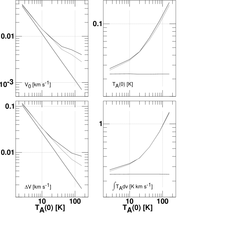
Figure 2: Rms error of derived gaussian fitting parameters. Top left, central velocity. Bottom left, the FWHM, $\Delta V$. Top right, the peak line strength. Bottom right, the profile integral. In each panel the uppermost curve is the empirically-determined rms and the bottommost curve the expected or reported rms, all for weighting by a constant profile variance. The middle curve is the parameter rms when weighting by the correct noise variance. For the other assumptions used to calculate these curves, see Sect. 2.5

The results of this experiment are reported in Fig. 2. The bottom curve in each panel is the rms of the fitted parameter given by analytic formulae, which coincides with the mean a posteriori error estimate returned by fitting software which assumes a constant profile rms. Stronger lines lead to linear improvements in fitting of the central velocity and width in this case, while the peak and profile integral fits are independent of strength; the fractional precision increases but fitting to the profile integral does not achieve higher precision than simply summing the channel values.

The uppermost curve in each panel is the actual rms of the parameter determination with weighting by a constant variance. The shaded (middle) curve is the rms with proper weighting; in this case, the fitting software returns accurate error estimates. Several phenomena are discernible in this diagram. There are irremediable increases in the variances of the fitted parameters relative to the case of constant profile rms. The precision of the fitted centroid and width improve only very slowly for strong signals, instead of linearly. Variances of the peak and integrated strengths increase in absolute terms as well. The fitting is only very slightly improved by correct weighting and the actual variances and the claimed error estimates diverge sharply if the behaviour of the noise is ignored. This could be misconstrued as implying that the stronger lines are less purely Gaussian.

2.6 Sensitivity of absorption measurements

Staring at a continuum source characterized by an antenna temperature ${\rm T}_{\rm A}$ = ${\rm T}_{\rm C}$ results in a system temperature ${\rm T}_{\rm sys}$= ${\rm T}_{\rm T}$+ ${\rm T}_{\rm C}$. If the continuum is extinguished by a pure scatterer characterized by optical depth $\tau(v)$, it follows that

$$\mbox{${\rm T}_{\rm sys}$}({\rm v})=\mbox{${\rm T}_{\rm T}$}+\mbox{${\rm T}_{\rm C}$}e^{-\tau(v)}$$

$$\mbox{$\Delta{\rm T}$}({\rm v})={{\mbox{${\rm T}_{\rm sys}$}({\rm v})}\over{\sqrt{{\rm N_{on}}}}}={{\mbox{${\rm T}_{\rm T}$}+\mbox{${\rm T}_{\rm C}$}e^{-\tau(v)}}\over{\sqrt{{\rm N_{on}}}}}$$

The system temperature is higher where there is no absorption. Eqn. 4 can be inverted to solve for the optical depth from the observed profile of ${\rm T}_{\rm sys}$(v), $i.e.$ $\tau(v)=-\ln{((\mbox{${\rm T}_{\rm sys}$}(v)-\mbox{${\rm T}_{\rm T}$})/\mbox{${\rm T}_{\rm C}$})}$. Neglecting other effects, the rms of the line/continuum ratio (the argument of the logarithm in this expression) is just $\sigma_{l/c}=\mbox{$\Delta{\rm T}$}/\mbox{${\rm T}_{\rm C}$}$. $\sigma_{l/c}$ may be normally distributed but the logarithmic dependence of $\tau(v)$ makes its error distribution noticeably asymmetric for moderate to large optical depth. Change in the derived optical depth for a given fluctuation $\delta_{l/c}$ in the line/continuum ratio can be written

$$\delta\tau(v)_{\mp}=\tau(v)+\ln{(e^{-\tau(v)}\pm\delta_{l/c})}$$

where $\pm$ and $\mp$ convey the sense of the variations. Differentiation yields the rms of the derived optical depth

$$\Delta\tau(v)=\sigma_{l/c}e^{\tau(v)}[{{\mbox{${\rm T}_{\rm T}$}+\mbox{${\rm T}_{\rm C}$}e^{-\tau(v)}}\over{\mbox{${\rm T}_{\rm T}$}+\mbox{${\rm T}_{\rm C}$}}}].$$

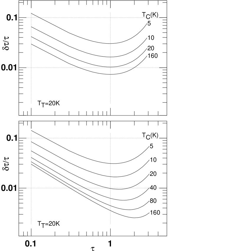
Figure 3: Fractional rms error in optical depth when a nominal 20 K system is used to observe continuum sources of varying strengths ${\rm T}_{\rm C}$, occulted by a pure scattering medium of optical depth $\tau$. These plots correspond roughly to 30 second integrations in 1 km s^-1 channels at 1420 MHz. At top, ${\rm T}_{\rm sys}$ is assumed independent of $\tau$; at bottom the dependence of ${\rm T}_{\rm sys}$ on $\tau$ (Eqn. 7) is included.

The usual analysis sets $\tau(v)=0$ on the right-hand side of Eqn. 5 so that the term in brackets in Eqn. 7 is unity. In Fig. 3 we plot $\delta\tau_{+}/\tau~{}vs.~{}\tau$ for different ${\rm T}_{\rm C}$, taking $\delta_{l/c}=\sigma_{l/c}$ in Eqn. 6 and assuming ${\rm T}_{\rm T}$= 20 K, $\sqrt{N}=376.9$ as before. In the usual analysis (upper panel) the fractional error in optical depth is minimized at $\tau\approx 1$ for all ${\rm T}_{\rm C}$ and sensitivity appears to saturate at rather small $\mbox{${\rm T}_{\rm C}$}\approx\mbox{${\rm T}_{\rm T}$}$. However, use of Eqn. 7 shows that the sensitivity never saturates, in the sense that it is possible to achieve higher precision on ever-thicker lines (lower panel). Furthermore, the error in optical depth at $\tau\approx 1$ is much smaller in the lower panel when ${\rm T}_{\rm C}$$>$ ${\rm T}_{\rm T}$.

Numerical experiments doing Gaussian fitting to absorption lines showed (as before) that proper weighting gives slightly improved parameter variances, and much-improved error estimates. Because the rms is higher in signal-free regions, naive error estimates returned by unwitting software are too large. Error in determining the continuum level of the baseline regions of an absorption spectrum increases with ${\rm T}_{\rm C}$ and may eventually become the limiting factor in determining the line/continuum ratio.

2.7 Quantization noise

Use of digital correlators represents a possible departure from the frequency-preserving character of the receiver and detector front-end, owing to the phenomenon of quantization noise (Bennett, 1948; Gwinn et al., 2000). Input to the correlator is bandpass filtered so that the sampling theorem may be applied to recovery of the data, but digitization of the continuously varying input power results in a representation of the signal which is very strongly not band-limited. That portion of the power spectrum lying outside the original band is returned, in varying degree depending on the sampling rate, as a form of noise. For Nyquist sampling (sampling at a rate twice the bandwidth) all is returned. For faster sampling the return is reduced as sampling sidebands beat with weaker, further-out portions of the quantization noise spectrum. As shown by Bennett (1948) for a 16-level system, quantization noise is steadily reduced until the sampling rate is 10 times Nyquist.

Thus, sampling and quantization schemes scatter input power throughout the passband. Experiments using input thermal noise on systems with (many) more bits than are used in radio astronomy show that the quantization noise is essentially white (ibid) but the spectral characteristics of quantization noise are very much dependent on the form of the input. Very strong, highly confined signals can produce distortions of the outlying passband. Weaker signals will simply be dispersed with little effect on either the noise level or shape of the passband.

Because of quantization noise, even the blackest absorption line will not reduce the rms to the level attained in the absence of all input signal. Eqn. 5, modified to account for quantization loss (1-$\epsilon$) in the case that strong absorption occupies a negligibly small fraction of the correlator bandpass (so that the quantization noise remains evenly distributed over the passband) is

$$\Delta{\rm T}={{\mbox{${\rm T}_{\rm T}$}+\mbox{${\rm T}_{\rm C}$}(\epsilon e^{-\tau}+(1-\epsilon))}\over{\epsilon\sqrt{\rm N}}}.$$

Examples of quantization losses at Nyquist sampling rates are (1-$\epsilon$) = 0.36 (1-bit or 2-level quantization), 0.12 (3-level) and 0.028 (9-level), so that minimum fractions $(1-\epsilon)/\epsilon$ = 0.57, 0.14 or 0.03 of the rms corresponding to the input ${\rm T}_{\rm C}$ would unavoidably be present in each channel, including those at the bottom of the line. This complicates error analysis but the high efficiencies of modern correlators preserve at least some of the benefits discussed. Such considerations are another reason to prefer higher-level quantization and over-sampling schemes.

3 Summary and extension to interferometry

Radio astronomers frequently observe signals which are strong enough to dominate the random errors of their experiments. Unfortunately, it is not always possible to recognize the effects which are induced and they are neglected. Nonetheless, they have always been present in the data.

This discussion points up obvious deficiencies in extant data reduction software and analysis techniques. Perhaps less obvious is the need not only for accurate calibration but also for reliable reporting on the part of the telescope systems. Measurement errors cannot be accurately assessed and accomodated in downstream data handling unless the system, continuum and line antenna temperatures are preserved, along with knowledge of the mode of data-taking. Synthesis instruments may be particularly difficult in this regard. Consider the use of the VLA (say) to detect H I absorption against a continuum source at low galactic latitude in the presence of an emission profile like that shown in Fig. 1. The VLA does not return the total power or singledish spectra, or, equivalently, the variation of ${\rm T}_{\rm sys}$ across the passband. The interferometer experiment per se can only succeed to the extent that foreground emission disappears; only its added noise contribution remains.

We began the discussion by pointing out that the noise contributed from sky signals in single-dish observations occurs – ignoring sidelobes, quantization noise and the like – at those places and/or frequencies where the sources themselves are located. It is an interesting endeavour to try to understand the extent to which source noise in interferometer experiments is similarly localized in the output datastream. For phased arrays it would seem possible to reproduce the single-dish mode. For synthesis arrays (Anantharamaiah et al., 1989; Crane & Napier, 1989) the situation is much more complicated and uncertain even in the weak signal limit.

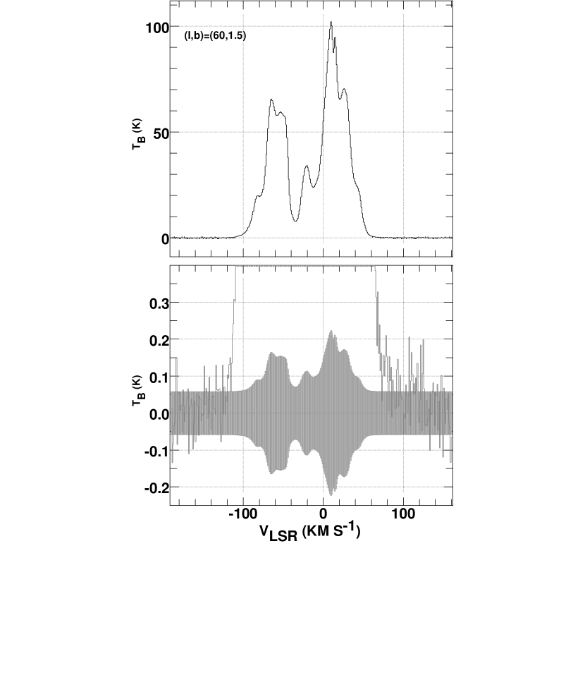
Figure 1: Top: H I emission observed at (l,b) = (60^o,$+$1.5^o) with the 25m Dwingeloo telescope by Hartmann & Burton (1997). Bottom: expanded view of the $\pm 1\sigma$ noise envelope assuming $\mbox{${\rm T}_{\rm T}$}=36$ K.

References

- Anantharamaiah et al. (1989) Anantharamaiah, K. R., Ekers, R. D., Radhakrishnan, V., Cornwell, T. J., & Goss, W. M. 1989, in ASP Conf. Ser. 6: Synthesis Imaging in Radio Astronomy, ed. R. A. Perley, F. R. Schwab, & A. H. Bridle, 431–442
- Bennett (1948) Bennett, W. R. 1948, BSTJ, 27, 446
- Burke & Graham-Smith (1997) Burke, B. F. & Graham-Smith, F. 1997, An Introduction to Radio Astronomy (Cambridge, U.K. ; New York : Cambridge University Press, 1997)
- Callen & Welton (1951) Callen, H. B. & Welton, T. A. 1951, Phys. Rev, 83, 1
- Crane & Napier (1989) Crane, P. C. & Napier, P. J. 1989, in ASP Conf. Ser. 6: Synthesis Imaging in Radio Astronomy, ed. R. A. Perley, F. R. Schwab, & A. H. Bridle, 139–165
- Dicke (1946) Dicke, R. 1946, Rev. Sci. Inst., 17, 268
- Gwinn et al. (2000) Gwinn, C. R., Carlson, B., Dougherty, S., Del Rizzo, D., Reynolds, J. E., Jauncey, D. L., Tzioumis, A. K., Quick, J., McCulloch, P. M., Hirabayashi, H., Kobayashi, H., & Y., M. 2000, astro-ph0002064
- Hartmann & Burton (1997) Hartmann, D. & Burton, W. B. 1997, Atlas of galactic neutral hydrogen (Cambridge, New York: Cambridge University Press.)
- Kaper et al. (1966) Kaper, H. G., Smits, D. W., Schwarz, U. J., Takakubo, K., & van Woerden, H. 1966, B. A. N., 18, 465
- Kraus (1986) Kraus, J. D. 1986, Radio astronomy (Powell, Ohio: Cygnus-Quasar Books, 1986)
- Marshall (1995) Marshall, J. 1995, Mon. Not. R. Astron. Soc., 275, 217
- Rieu (1969) Rieu, N. 1969, A&A, 1, 128
- Rohlfs et al. (2000) Rohlfs, K., Wilson, T. L., & Huettemeister, S. 2000, Tools of radio astronomy (New York : Springer, 2000. (Astronomy and astrophysics Library))