Radiative Transfer with Finite Elements

A finite element method for solving the resonance line transfer problem in moving media is presented. The algorithm works in three spatial dimensions on unstructured grids which are adaptively refined by means of an a posteriori error indicator. Frequency discretization is implemented via a first-order Euler scheme. We discuss the resulting matrix structure for coherent isotropic scattering and complete redistribution. The solution is performed using an iterative procedure, where monochromatic radiative transfer problems are successively solved. The present implementation is applicable for arbitrary model configurations with an optical depth up to $10^{3-4}$. Results of Ly$\alpha$ line transfer calculations for a spherically symmetric model, a disk-like configuration, and a halo containing three source regions are discussed. We find the characteristic double-peaked Ly$\alpha$ line profile for all models with an optical depth $\ga 1$. In general, the blue peak of the profile is enhanced for models with infall motion and the red peak for models with outflow motion. Both velocity fields produce a triangular shape in the two-dimensional Ly$\alpha$ spectra, whereas rotation creates a shear pattern. Frequency-resolved Ly$\alpha$ images may help to find the number and position of multiple Ly$\alpha$ sources located in a single halo. A qualitative comparison with observations of extended Ly$\alpha$ halos associated with high redshift galaxies shows that even models with lower hydrogen column densities than required from profile fitting yield results which reproduce many features in the observed line profiles and two-dimensional spectra.

1 Introduction

Hydrogen Ly$\alpha$ as a prominent emission line of high redshift galaxies is important for the understanding of galaxy formation and evolution in the early universe. Recent narrow-band imaging and spectroscopic surveys used the Ly$\alpha$ line to identify galaxies at very high redshift (e.g. Hu et al. hu:etal98 (1998); Kudritzki et al. kudritzki:etal2000 (2000); Rhoads et al. rhoads:etal2000 (2000); Fynbo et al. fynbo:etal2000 (2000), fynbo:etal2001 (2001)).

But beside from being a good redshift indicator, Ly$\alpha$ emission also bears information on the distribution and kinematics of the interstellar gas as well as the nature of the energy source. Ly$\alpha$ observations of high redshift radio galaxies (e.g. Hippelein & Meisenheimer hippelein:meisenheimer93 (1993); van Ojik et al. vanojik:etal96 (1996), vanojik:etal97 (1997); Villar-Martín et al. villar-martin:etal99 (1999)) reveal extended Ly$\alpha$ halos with sizes $>100$ kpc which are aligned with the radio jet. The line profiles are often double-peaked and the two-dimensional spectra point to complex kinematics involving velocities $>1000$ km$\;\mbox{s}^{-1}$.

The interpretation of Ly$\alpha$ observations is difficult, because high-redshift radio galaxies tend to be in the center of proto clusters, where the radio jet interacts with a clumpy environment influenced by merging processes (e.g. Bicknell et al. bicknell:etal2000 (2000); Kurk et al. kurk:etal2001 (2001)). Actually, the three-dimensional structure of the objects and the fact that Ly$\alpha$ is a resonance line require detailed radiative transfer modeling.

The transfer of resonance line photons is profoundly determined by scattering in space and frequency. Analytical (Neufeld neufeld90 (1990)) as well as early numerical methods (Adams adams72 (1972); Hummer & Kunasz hummer:kunasz80 (1980)) were restricted to one-dimensional, static media. Only recently, codes based on the Monte Carlo method were developed which are capable to investigate the more general case of a multi-dimensional medium (Ahn et al. ahn:etal2001 (2001), ahn:etal2002 (2002)).

In this paper, we introduce a finite element method for the solution of the resonance line transfer problem in three-dimensional, moving media and present the results of some simple, slightly optically thick model configurations. The basic, monochromatic code was originally developed by Kanschat (kanschat96 (1996)) and is described in Richling et al. (richling:etal2001 (2001), hereafter Paper I). The three-dimensional method is particularly useful for scattering dominated problems in inhomogeneous media. Steep gradients are resolved by means of an adaptively refined grid. Here, we only specify the extension from the monochromatic to the polychromatic problem including the implementation of the Doppler-effect and complete redistribution.

In Sect. 2, we review the equations for resonance line transfer in moving media. In Sect. 3, we describe some details regarding frequency discretization and the form of the resulting matrices for coherent scattering and complete redistribution and give a short outline of the complete finite element algorithm. Then, the results of a spherically symmetric model (Sect. 4), a disk-like configuration (Sect. 5) and a model with three separate source regions (Sect. 6) are presented. A summary is given in Sect. 7.

2 Line Transfer in Moving Media

We calculate the frequency-dependent radiation field in moving media by solving the non-relativistic radiative transfer equation in the comoving frame for a three-dimensional domain $\Omega$ which in operator form simply reads

$$\bigl{(}{\cal T}+{\cal D}+{\cal S}+\chi({\bf x},\nu)\bigr{)}{\cal I}({\bf x},{\bf n},\nu)=f({\bf x},\nu).$$ (1)

The transfer operator ${\cal T}$, the “Doppler” operator ${\cal D}$, and the scattering operator ${\cal S}$ are defined by

$${\cal T}{\cal I}({\bf x},{\bf n},\nu)={\bf n}\cdot\nabla_{x}{\cal I}({\bf x},{\bf n},\nu),$$

$${\cal D}{\cal I}({\bf x},{\bf n},\nu)=w({\bf x},{\bf n})\,\nu\frac{\partial}{\partial\nu}{\cal I}({\bf x},{\bf n},\nu),$$

$${\cal S}{\cal I}({\bf x},{\bf n},\nu)=-\frac{\sigma({\bf x})}{4\pi}\int_{0}^{\infty}\int_{S^{2}}R(\hat{{\bf n}},\hat{\nu};{\bf n},\nu){\cal I}({\bf x},\hat{{\bf n}},\hat{\nu})\,d\hat{\omega}\,d\hat{\nu}.$$

Considering three dimensions in space, the relativistic invariant specific intensity ${\cal I}$ is six-dimensional and depends on the space variable ${\bf x}$, the direction ${\bf n}$ (pointing to the solid angle $d\omega$ of the unit sphere $S^{2}$), and the frequency $\nu$.

The extinction coefficient $\chi({\bf x},\nu)=\kappa({\bf x},\nu)+\sigma({\bf x},\nu)$ is the sum of the absorption coefficient $\kappa({\bf x},\nu)=\kappa({\bf x})\phi(\nu)$ and the scattering coefficient $\sigma({\bf x},\nu)=\sigma({\bf x})\phi(\nu)$. The frequency-dependence is given by a normalized profile function $\phi$. Usually, we adopt a Doppler profile

$$\phi(\nu)=\frac{1}{\sqrt{\pi}\,\Delta\nu_{D}}\exp{\left[-\left(\frac{\nu-\nu_{0}}{\Delta\nu_{D}}\right)^{2}\right]},$$ (2)

where $\nu_{0}$ is the frequency of the line center. The Doppler width $\Delta\nu_{D}$ and the Doppler velocity $v_{D}$ are determined by a thermal velocity $v_{\rm therm}$ as well as a turbulent velocity $v_{\rm turb}$

$$\Delta\nu_{D}=\frac{\nu_{0}}{c}v_{D}=\frac{\nu_{0}}{c}\sqrt{v_{\rm therm}^{2}+v_{\rm turb}^{2}}.$$ (3)

$c$ is the speed of light. For situations, where $v_{\rm turb}\gg v_{\rm therm}$, the Doppler core is very broad and would dominate the Lorentzian wings of a Voigt profile. Then, the Doppler profile is a reasonable description of a line profile. Throughout this paper we use $v_{D}=10^{-3}c\sim 300\;\mbox{km}\,\mbox{s}^{-1}$ (see also Table 1).

For the source term

$$f({\bf x},\nu)=\kappa({\bf x},\nu)B(T({\bf x}),\nu)+\epsilon({\bf x},\nu),$$ (4)

we can consider thermal radiation and non-thermal radiation. In the case of thermal radiation, $f$ is calculated from a temperature distribution $T({\bf x})$, where $B(T,\nu)$ is the Planck function.

The “Doppler” operator ${\cal D}$ is responsible for the Doppler shift of the photons. A derivation of the operator for non-relativistic velocities ($v/c<0.1$) can be found in Wehrse et al. (wehrse:etal2000 (2000)). In contrast to the full relativistic transfer equation (cf. Mihalas & Weibel-Mihalas mihalas:weibel-mihalas84 (1984)), we neglect any terms responsible for aberration or advection effects. The function

$$w({\bf x},{\bf n})=-{\bf n}\cdot\nabla_{x}\left({\bf n}\cdot\frac{{\bf v}({\bf x})}{c}\right)$$ (5)

is the gradient of the velocity field ${\bf v}({\bf x})$ in direction ${\bf n}$. Note that the sign of $w$ may change depending on the complexity of the velocity field ${\bf v}$.

The scattering operator ${\cal S}$ depends on the general redistribution function $R(\hat{{\bf n}},\hat{\nu};{\bf n},\nu)$ giving the probability that a photon $(\hat{{\bf n}},\hat{\nu})$ is absorbed and a photon $({\bf n},\nu)$ is emitted. In the following, we assume isotropic scattering

$${\cal S}{\cal I}=-\frac{\sigma({\bf x})}{4\pi}\int\limits_{0}^{\infty}R(\hat{\nu},\nu)\int_{S^{2}}{\cal I}({\bf x},\hat{{\bf n}},\hat{\nu})\,d\hat{\omega}\,d\hat{\nu},$$ (6)

where $R(\hat{\nu},\nu)$ is the angle-averaged redistribution function

$$R(\hat{\nu},\nu)=\frac{1}{(4\pi)^{2}}\int_{S^{2}}\int_{S^{2}}R({\bf x},\hat{{\bf n}},\hat{\nu};{\bf n},\nu)\,d\hat{\omega}\,d\omega.$$ (7)

The function defined by (7) is normalized such that

$$\int\limits_{0}^{\infty}\int\limits_{0}^{\infty}R(\hat{\nu},\nu)\,d\hat{\nu}\,d\nu=1.$$ (8)

For the calculations in Sect. 3, we consider two limiting cases: strict coherence and complete redistribution in the comoving frame. In the former case, we have

$$R(\hat{\nu},\nu)=\phi(\hat{\nu})\delta(\nu-\hat{\nu})$$ (9)

and in the latter

$$R(\hat{\nu},\nu)=\phi(\hat{\nu})\phi(\nu).$$ (10)

Thus, for coherent isotropic scattering, the scattering term simplifies to

$${\cal S}^{\rm coh}{\cal I}({\bf x},{\bf n},\nu)=-\frac{\sigma({\bf x},\nu)}{4\pi}\int_{S^{2}}{\cal I}({\bf x},\hat{{\bf n}},\nu)\,d\hat{\omega}$$ (11)

In the case of complete redistribution, the photons are scattered isotropically in angle, but are randomly redistributed over the line profile. Then, the scattering term reads

$${\cal S}^{\rm crd}{\cal I}({\bf x},{\bf n},\nu)=-\frac{\sigma({\bf x},\nu)}{4\pi}\int_{0}^{\infty}\phi(\hat{\nu})\int_{S^{2}}{\cal I}({\bf x},\hat{{\bf n}},\hat{\nu})\,d\hat{\omega}\,d\hat{\nu}.$$ (12)

3 The Finite Element Method

3.1 Boundary Conditions

For the modeling of prominent resonance lines, in particular Ly$\alpha$, we restrict the frequency discretization to a finite interval $\Lambda:=[\nu_{0},\nu_{N+1}]$, where $\nu_{0}$ and $\nu_{N+1}$ are located far out of the line center in the continuum. The function $w({\bf x},{\bf n})$ from Eq. (5) defines the Doppler shift of the spectrum towards smaller ($w<0$) or larger ($w>0$) frequencies in the comoving frame. Therefore, boundary conditions of the form

$${\cal I}({\bf x},{\bf n},\nu)={\cal I}_{\rm cont}({\bf x},{\bf n},\nu)$$

are necessary on the upper and lower frequency interval boundary of the whole computational domain

$$\Sigma=\Omega\times{\cal S}^{2}\times\{\nu_{0},\nu_{N+1}\}.$$

Furthermore, to be able to solve Eq. (1), boundary conditions of the form

$${\cal I}({\bf x},{\bf n},\nu)={\cal I}_{\rm in}({\bf x},{\bf n},\nu)$$

must be imposed on the “inflow boundary”

$$\Gamma^{-}\times\Lambda=\bigl{\{}({\bf x},{\bf n},\nu)\in\Gamma|\mbox{\,}{\bf n}_{\Gamma}\cdot{\bf n}<0\bigr{\}},$$

where ${\bf n}_{\Gamma}$ is the unit vector perpendicular to the boundary surface $\Gamma$ of the spatial domain $\Omega$. The sign of the product ${\bf n}_{\Gamma}\cdot{\bf n}$ describes the “flow direction” of the photons across the boundary. If we neglect any continuum emission (${\cal I}_{\rm cont}=0$) and assume that there are no light sources outside the modeled domain as in the case of a non-illuminated atmosphere (${\cal I}_{\rm in}=0$), the two boundary conditions for the solution of the transfer equation (1) in moving media are

$${\cal I}({\bf x},{\bf n},\nu) =0\mbox{\qquad on }\;\Sigma,$$ (13)

$${\cal I}({\bf x},{\bf n},\nu) =0\mbox{\qquad on }\;\Gamma^{-}\times\Lambda.$$ (14)

3.2 Discretization for Coherent Scattering

In order to solve the radiative transfer equation (1), we first carry out the frequency discretization including coherent scattering. With the abbreviation

$${\cal A}^{\rm coh}={\cal T}+{\cal S}^{\rm coh}+\chi({\bf x},\nu)$$ (15)

Eq. (1) can be written as

$${\cal A}^{\rm coh}{\cal I}({\bf x},{\bf n},\nu)+w({\bf x},{\bf n})\nu\frac{\partial}{\partial\nu}{\cal I}({\bf x},{\bf n},\nu)=f({\bf x},\nu).$$ (16)

In Paper I, we described a Galerkin discretization for the monochromatic radiative transfer equation. Considering memory and CPU requirements this approach is by far too “expensive” for the frequency-dependent transfer problem. Instead, we use an implicit Euler method for $N$ equidistantly distributed frequency points $\nu_{i}\in\bigl{\{}\nu_{1},\nu_{2},...,\nu_{N}\bigr{\}}\subset\Lambda$. Since the function $w({\bf x},{\bf n})$ may change its sign, this simple difference scheme for the Doppler term reads

$$w({\bf x},{\bf n})\nu\frac{\partial{\cal I}}{\partial\nu} \longrightarrow w\nu_{i}\frac{{\cal I}_{i}-{\cal I}_{i-1}}{\Delta\nu}\mbox{\qquad}(w_{i}>0)$$ (17)

and

$$w({\bf x},{\bf n})\nu\frac{\partial{\cal I}}{\partial\nu} \longrightarrow w\nu_{i}\frac{{\cal I}_{i+1}-{\cal I}_{i}}{\Delta\nu}\mbox{\qquad}(w_{i}<0),$$ (18)

where $\Delta\nu$ is the constant frequency step size. All quantities referring to the discrete frequency point $\nu_{i}$ are denoted by an index “$i$”. Employing the Euler method, we get a semi-discrete representation of Eq. (16)

$$\Bigl{(}{\cal A}_{i}^{\rm coh}+\frac{|w|\nu_{i}}{\Delta\nu}\Bigr{)}{\cal I}_{i}=f_{i}+\frac{|w|\nu_{i}}{\Delta\nu}\left\{\begin{array}[]{r@{\quad}l}{\cal I}_{i-1}&(w>0)\\ {\cal I}_{i+1}&(w<0)\end{array}\right..$$ (19)

The additional term on the left side of Eq. (19) can be interpreted as an artificial opacity, which is advantageous for the solution of the resulting linear system of equations. The additional term on the right side of Eq. (19) is included as an artificial source term. Equation (19) can be written in a compact operator form

$$\tilde{{\cal A}}_{i}^{\rm coh}{\cal I}_{i}=\tilde{f_{i}}.$$ (20)

Given a discretization with $L$ degrees of freedom in $\Omega$, $M$ directions on the unit sphere $S^{2}$ and $N$ frequency points, the overall discrete system has the matrix form

$${\bf A}^{\rm coh}{\bf u}={\bf f},$$ (21)

with the vector ${\bf u}$ containing the discrete intensities and the vector ${\bf f}$ the values of the source term for all frequency points $\nu_{i}$. Both vectors are of length $(L\cdot M\cdot N)$ and ${\bf A}^{\rm coh}$ is a $(L\cdot M\cdot N)\times(L\cdot M\cdot N)$ matrix. The fact that the function $w({\bf x},{\bf n})$ may change its sign, results in a block-tridiagonal structure of ${\bf A}^{\rm coh}$ and we get

$$\begin{array}[]{cccc}\left(\begin{array}[]{ccccc}{\tilde{\bf A}}_{1}^{\rm coh}&{\bf R}_{1}&{\bf 0}&\ldots&{\bf 0}\\ {\bf B}_{2}&{\tilde{\bf A}}_{2}^{\rm coh}&{\bf R}_{2}&\ddots&\vdots\\ {\bf 0}&\ddots&\ddots&\ddots&{\bf 0}\\ \vdots&\ddots&\ddots&\ddots&{\bf R}_{N-1}\\ {\bf 0}&\ldots&{\bf 0}&{\bf B}_{N}&{\tilde{\bf A}}_{N}^{\rm coh}\end{array}\right)&\left(\begin{array}[]{c}{\bf u}_{1}\\ {\bf u}_{2}\\ \vdots\\ \vdots\\ {\bf u}_{N}\end{array}\right)&=&\left(\begin{array}[]{c}{\bf f}_{1}\\ {\bf f}_{2}\\ \vdots\\ \vdots\\ {\bf f}_{N}\end{array}\right).\end{array}$$

According to the sign of $w({\bf x},{\bf n})$ the block matrices ${\bf R}_{i}$ and ${\bf B}_{i}$ hold entries of $w({\bf x},{\bf n})\nu_{i}/\Delta\nu$ causing a redshift and blueshift of the photons in the medium, respectively. Requiring a reasonable resolution, the resulting linear system of equations of the total system is too large to be solved directly. Hence, we are treating $N$ “monochromatic” radiative transfer problems

$${\tilde{\bf A}}_{i}^{\rm coh}{\bf u}_{i}=\tilde{{\bf f}}_{i},$$ (22)

with a slightly modified right hand side

$$\tilde{{\bf f}}_{i}={\bf f}_{i}+{\bf R}_{i}{\bf u}_{i+1}+{\bf B}_{i}{\bf u}_{i-1}.$$ (23)

Note that using simple velocity fields (e.g. infall or outflow) the sign of $w({\bf x},{\bf n})$ is fixed and the matrix ${\bf A}^{\rm coh}$ has a block-bidiagonal structure. This is favorable for our solution strategy, since we only need to solve Eq. (22) once for each frequency.

3.3 Discretization for Complete Redistribution

Considering complete redistribution, we use an implicit Euler scheme to discretize the Doppler term as described above and a simple quadrature method for the frequency integral in the scattering operator ${\cal S}^{\rm crd}$ in Eq. (12). Starting from $N$ equidistantly distributed frequency points $\nu_{i}\in\bigl{\{}\nu_{1},\nu_{2},...,\nu_{N}\bigr{\}}\subset\Lambda$ and $N$ weights $q_{1},q_{2},...,q_{N}$, we define a quadrature method

$$Q(\nu_{i}):=\sum_{j=1}^{N}q_{j}\xi(\nu_{j})$$ (24)

for integrals $\int_{\Lambda}\xi(\nu^{\prime})d\nu^{\prime}$. In the case of complete redistribution the kernel is

$$\xi(\nu_{j})=\frac{\phi(\nu_{j})}{4\pi}\int_{S^{2}}{\cal I}({\bf x},\hat{{\bf n}},\nu_{j})d\hat{\omega}.$$ (25)

Separating the terms with the unknown intensities ${\cal I}_{i}$ from the known quantities ${\cal I}_{j}$ the discretized scattering integral (12) reads

$$\frac{\sigma_{i}}{4\pi}\phi_{i}q_{i}\int_{S^{2}}{\cal I}_{i}d\hat{\omega}+\frac{\sigma_{i}}{4\pi}\sum_{j\not=i}^{N}\phi_{j}q_{j}\int_{S^{2}}{\cal I}({\bf x},\hat{{\bf n}},\nu_{j})d\hat{\omega}.$$ (26)

Using this quadrature scheme and employing the Euler method for the frequency derivatives we get a semi-discrete formulation of the transfer problem for each frequency point including complete redistribution

$$\Bigl{(}{\cal A}^{\rm crd}_{i}+\frac{|w|\nu_{i}}{\Delta\nu}\Bigr{)}{\cal I}_{i}\\ \mbox{\hfill}=\tilde{f}_{i}+\frac{\sigma_{i}}{4\pi}\sum_{j\not=i}^{N}\phi_{j}q_{j}\int_{S^{2}}{\cal I}({\bf x},\hat{{\bf n}},\nu_{j})d\hat{\omega},$$ (27)

where

$${\cal A}^{\rm crd}_{i}={\cal T}+\chi_{i}+\phi_{i}q_{i}{\cal S}^{\rm coh}.$$ (28)

The additional terms on the right hand side of Eq. (27) must be interpreted as artificial source terms. Eq. (27) can also be written in a compact operator form

$$\tilde{{\cal A}}_{i}^{\rm crd}{\cal I}_{i}=\hat{f_{i}}.$$ (29)

The total discrete system has the matrix form (cf. Eq. (21))

$${\bf A}^{\rm crd}{\bf u}={\bf f}.$$ (30)

Unfortunately, the global frequency coupling via the scattering integral (12) results in a full block matrix and we get

$$\begin{array}[]{ccc}{\bf A}^{\rm crd}&=&\left(\begin{array}[]{ccccc}{\tilde{\bf A}}_{1}^{\rm crd}&{\bf R}_{1}+{\bf Q}_{2}&{\bf Q}_{3}&\ldots&{\bf Q}_{N}\\ {\bf B}_{2}+{\bf Q}_{1}&{\tilde{\bf A}}_{2}^{\rm crd}&{\bf R}_{2}+{\bf Q}_{3}&\ddots&\vdots\\ {\bf Q}_{1}&\ddots&\ddots&\ddots&\vdots\\ \vdots&\ddots&\ddots&\ddots&\vdots\\ {\bf Q}_{1}&\ldots&\ldots&\ldots&{\tilde{\bf A}}_{N}^{\rm crd}\end{array}\right).\end{array}$$

${\bf B}_{i}$ and ${\bf R}_{i}$ again contain the contribution of the Doppler factor $w({\bf x},{\bf n})\nu_{i}/\Delta\nu$, whereas ${\bf Q}_{j}$ holds the terms from the quadrature scheme. As we already explained in the case of coherent scattering, we do not solve the total system, but $N$ “monochromatic” radiative transfer problems

$${\tilde{\bf A}}_{i}^{\rm crd}{\bf u}_{i}=\hat{{\bf f}}_{i},$$ (31)

with a modified right hand side

$$\hat{{\bf f}}_{i}={\bf f}_{i}+{\bf R}_{i}{\bf u}_{i+1}+{\bf B}_{i}{\bf u}_{i-1}+\sum_{j\not=i}{\bf Q}_{j}{\bf u}_{j}.$$ (32)

3.4 Full Solution Algorithm

Eq. (20) and (29) are of the same form as the monochromatic radiative transfer equation, ${\cal A}{\cal I}=f$, for which we proposed a solution method based on a finite element technique in Paper I. The finite element method employs unstructured grids which are adaptively refined by means of an a posteriori error estimation strategy. Now, we apply this method to Eq. (20) or Eq. (29). In brief, the full solution algorithm reads:

1. Start with ${\cal I}=0$ for all frequencies.

2. Solve Eq. (20) or Eq. (29) for $i=1,..,N$.

3. Repeat step 2 until convergence is reached.

4. Refine grid and repeat step 2 and 3.

We start with a relatively coarse grid, where only the most important structures are pre-refined, and assure that the frequency interval $[\nu_{1},\nu_{N}]$ is wide enough to cover the total line profile. Then, we solve Eq. (20) or Eq. (29) for each frequency several times depending on the choice of the redistribution function and the velocity field. During this fix point iteration, we monitor the changes of the resulting line profile in a particular direction ${\bf n}_{\rm out}$. Not until the line profile remains unchanged, we go over to step 4 and refine the spatial grid. Again, we apply the fixed fraction grid refinement strategy: The cells are ordered according to the size of the local refinement indicator $\eta_{K}=max(\eta_{K}(\nu_{i}))|_{\nu_{i}}$ and a fixed portion of the cells with largest $\eta_{K}$ is refined. $\eta_{K}(\nu_{i})$ is an indicator for the error of the solution in cell $K$ at frequency $\nu_{i}$.

In Paper I (Sect. 2.3), we introduced various possibilities to determine $\eta_{K}$. If we use the total flux leaving the computational domain in direction ${\bf n}_{\rm out}$ as the quantity whose error functional is used to calculate $\eta_{K}$ (dual method), our convergence criterion described above is perfectly reasonable. We found that this criterion is also useful for the much simpler method (L² method), where $\eta_{K}$ is determined from the global error functional. In this case, the rate of convergence of the line profile in the directions ${\bf n}\neq{\bf n}_{\rm out}$ and for the line profile in direction ${\bf n}_{\rm out}$ are very similar. We are aware that this result may not be valid for more complex model configuration.

4 Model Configurations

4.1 Halo and Sources

We investigate spherically symmetric and elliptical distributions of the extinction coefficient $\chi({\bf x})=\chi(x,y,z)$ of the form

$$\chi({\bf x})=\left\{\begin{array}[]{ll}\chi_{0}/(1+\alpha r_{c}^{2})&\quad\mbox{for}\;r\leq r_{c}\\ \chi_{0}/(1+\alpha r^{2})&\quad\mbox{for}\;r_{c}<r\leq r_{h}\\ \chi_{0}/(1+\alpha r_{h}^{2})/10^{3}&\quad\mbox{for}\;r>r_{h}\end{array}\right.,$$ (33)

where $r^{2}=(x/a)^{2}+(y/b)^{2}+(z/c)^{2}$. Note, that the value of the extinction coefficient is constant in the center within core radius $r_{c}$ and outside halo radius $r_{h}$. If not stated otherwise, $\chi_{0}$ is determined from the line center optical depth

$$\tau=\int_{r_{c}}^{r_{h}}\chi(r)\phi(\nu_{0})\;{\bf n}_{\rm thick}\,d{\bf x}$$ (34)

between $r_{c}$ and $r_{h}$ along the most optically thick direction ${\bf n}_{\rm thick}$. In total, the spatial distribution of $\chi$ is determined by six parameters: the length of the half-axes $a$, $b$ and $c$, the radii $r_{c}$ and $r_{h}$, the dimensionless parameter $\alpha$, and the optical depth $\tau$. For $r_{c}$, $r_{h}$ and $\alpha$ we use the values given in Table 1.

Since we are predominantly interested in the transfer of radiation in resonance lines like Ly$\alpha$, we assume $\sigma({\bf x})=\chi({\bf x})$ and $\kappa({\bf x})=0$ for all calculation presented here. This restricts us to the use of purely non-thermal source functions. In particular, we consider one or several spatially confined source regions with radius $r_{s}$ each centered at a position ${\bf x}_{i}$:

$$f({\bf x},\nu)=\left\{\begin{array}[]{lr}\phi(\nu)&\quad\mbox{for}\quad|{\bf x}-{\bf x}_{i}|\leq r_{s}\\ 0&\quad\mbox{for}\quad|{\bf x}-{\bf x}_{i}|>r_{s}\end{array}\right..$$ (35)

The function $\phi(\nu)$ is the Doppler profile defined in Eq. (2).

4.2 Velocity Fields

In general, the finite element code is able to consider arbitrary velocity fields. For velocity fields defined on a discrete grid, for example for velocity fields resulting from hydrodynamical simulations, the velocity gradient in direction ${\bf n}$ must be obtained numerically. Here, we use two simple velocity fields and calculate the function $w$ analytically.

The first velocity field describes a spherically symmetric inflow ($v_{0}<0$) or outflow ($v_{0}>0$) and is of the form

$${\bf v}_{\rm io}=v_{0}\left(\frac{r_{0}}{r}\right)^{l}\frac{{\bf x}}{r},$$ (36)

where $r=|{\bf x}|$ and $v_{0}$ the scalar velocity at radius $r_{0}$. The corresponding $w$ function is

$$w({\bf x},{\bf n})=v_{0}\left(\frac{r_{0}}{r}\right)^{l}\left(\frac{1}{r}-(l+1)\frac{|{\bf n}{\bf x}|}{r^{3}}\right).$$ (37)

For the second velocity field, we assume rotation around the $z$-axis

$${\bf v}_{\rm rot}=v_{0}\left(\frac{R_{0}}{R}\right)^{l}R^{-1}\left(\begin{array}[]{rrr}y\\ -x\\ 0\end{array}\right),$$ (38)

where $R^{2}=x^{2}+y^{2}$ is the distance from the rotational axis and $v_{0}$ the scalar velocity at distance $R_{0}$. If ${\bf n}=(n_{x},n_{y},n_{z})$, the $w$ function reads

$$w=v_{0}\left(\frac{R_{0}}{R}\right)^{l}(l+1)\left(\frac{xy(n_{y}^{2}-n_{x}^{2})+n_{x}n_{y}(x^{2}-y^{2})}{R^{3}}\right).$$ (39)

In the special case of a Keplerian velocity field ($l=0.5$), we obtain

$$w=v_{0}\frac{3}{2}R_{0}^{0.5}R^{-3.5}\left[xy(n_{y}^{2}-n_{x}^{2})+n_{x}n_{y}(x^{2}-y^{2})\right]$$ (40)

(see also Baschek & Wehrse baschek:wehrse99 (1999)). Again, the values used for $v_{0}$, $r_{0}$ and $R_{0}$ are given in Table 1.

4.3 Normalization

Since we use a normalized form of the equation of transfer, where the computational domain is the unit cube, the results are valid for model configurations with different length scales and for different resonance lines. When $2x_{\max}$ is the size of the unit cube, coordinates in physical units are simply obtained by the transformation ${\bf x}\rightarrow{\bf x}\cdot x_{\rm max}$.

A particular line and the corresponding frequency scale must be defined when transforming to the observers frame. From the solution ${\cal I}({\bf x},{\bf n},\nu)$ in the comoving frame, we obtain the solution $\tilde{{\cal I}}({\bf x},{\bf n},\tilde{\nu})$ in the observers frame by performing the transformation

$$\tilde{{\cal I}}(x,{\bf n},\tilde{\nu})={\cal I}({\bf x},{\bf n},\tilde{\nu})\left(\frac{\tilde{\nu}}{\nu}\right)^{3},$$ (41)

where

$$\tilde{\nu}=\nu\left(1+{\bf n}\cdot\frac{{\bf v}({\bf x})}{c}\right).$$ (42)

The relation between optical depth $\tau$ and column density of the scattering media depends on the central line absorption cross section $\chi(\nu_{0})$ and therefore on the Doppler velocity $v_{D}$. For the Ly$\alpha$ line of neutral hydrogen the central line absorption cross section is

$$\chi_{{\rm Ly}\alpha}=2.0\times 10^{-15}\;\left(\frac{300\;\mbox{km}\,\mbox{s}^{-1}}{v_{D}}\right)\;\mbox{cm}^{2}\;.$$ (43)

Hence, the column density of neutral hydrogen for a halo with given $\tau$ is

$$N_{\rm H}=0.5\times 10^{14}\;\tau\;\left(\frac{v_{D}}{300\;\mbox{km}\,\mbox{s}^{-1}}\right)\;\mbox{cm}^{-2}.$$ (44)

We would like to emphasize that this value is the column density of the neutral halo alone. Considering the column density of the source region, the total column density is about twice as high and is in the range $N_{\rm H}\sim[10^{13},10^{16}]\;\mbox{cm}^{-2}$ for the investigated configurations with $\tau=[0.1,100]$.

In comparison to column densities deduced from Voigt profile fitting procedures of Ly$\alpha$ profiles of high redshift radio galaxies (van Ojik et al. vanojik:etal97 (1997)), our values are at least an order of magnitude too low. With the present implementation of our finite element code, we could calculate systems with column densities up to $N_{\rm H}\sim 10^{17}-10^{18}\;\mbox{cm}^{-2}$, but only with a large amount of computational time. Still higher column densities are beyond feasibility.

Table 1: Parameters used for all calculations. Distances are given in units of the computational cube (see Sect. 4.3).

$r_{h}$	$r_{c}$	$\alpha$	$r_{s}$	$v_{D}$	$v_{0}$	$r_{0}$	$R_{0}$
1.0	0.2	$10^{3}$	0.2	$10^{-3}c$	$-10^{-3}c$	0.2	1.0

Figure 1: Ly$\alpha$ line profiles calculated with the FE code for a spherically symmetric model configuration: a) a static halo with coherent scattering, b) an infalling halo with coherent scattering, c) a static halo with complete redistribution, and d) an infalling halo with complete redistribution. For the static cases a) and c) the line styles refer to calculations with different optical depth $\tau$ as indicated. The small window in a) enlarges the peak of the line. The crosses mark the results of the analytical solution. For the moving halos we show in b) the results for $\tau=1$ (thin lines) and $\tau=10$ (thick lines) and in d) only for $\tau=10$. Here, the line styles refer to the exponent $l$ used for the velocity fields.

Figure 2: Results obtained for a static, disk-like model configuration: a) Emergent line profiles for different viewing angles and optical depths $\tau=\tau({\bf n}_{\rm thick})$. b) Two-dimensional spectra for an edge-on view (90^∘) and a nearly face-on view (20^∘) and different optical depths. The position and width of the slit is indicated in Fig. 3a. The contours are given for 2.5%, 5%, 7.5%, 10%, 20%, …, 90% of the maximum value.

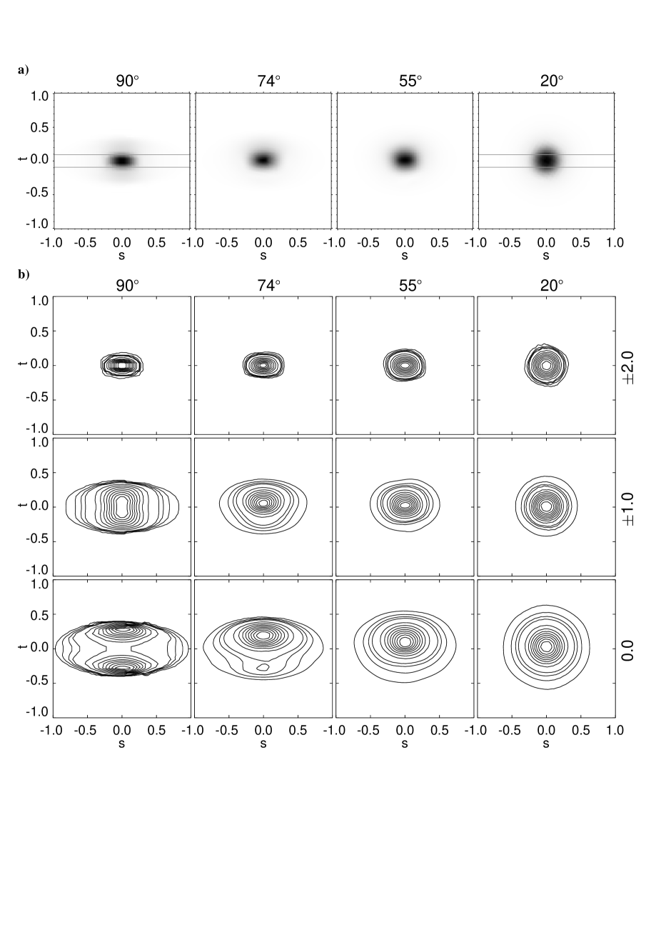
Figure 3: Spatial intensity distribution for a static disk-like model configuration with $\tau({\bf n}_{\rm thick})=10$ for different viewing angles: a) Frequency integrated intensity distribution. b) Intensity distribution for specific frequencies. The frequency is given in Doppler units relative to the line center $(\nu-\nu_{0})/\Delta\nu_{\rm D}$ at the right hand side.

5 Test calculations

We start with a spherically symmetric model configuration ($a=b=c=1$) and a single source region located at ${\bf x}=0$. Fig. 1 shows the results of the finite element code (FE code) for different optical depths, velocity fields and redistribution functions. We used 41 frequencies equally spaced in the interval $(\nu-\nu_{0})/\Delta\nu_{D}=[-4,6]$ and 80 directions. Starting with a grid of $4^{3}$ cells and a pre-refined source region, we needed 3–5 spatial refinement steps.

The simplest case is a static model with coherent isotropic scattering. Fig. 1a displays the emergent line profiles for different $\tau$. As expected, the Doppler profile is preserved and the flux $F_{\nu}$ is independent on $\tau$. The deviation of the numerical results from the analytical solution indicated with crosses is very small. The line profiles for $\tau=0.1$ and $\tau=1$ are identical even in the little window which shows the peak of the line in more detail. For $\tau=100$, the total flux is still conserved better than 99%. This result demonstrates that the frequency-dependent version of our FE code works correctly.

Next, we consider an infalling halo with coherent scattering and show the effects of frequency coupling due to the Doppler term. The emergent line profiles in Fig. 1b are plotted for different exponents $l$ of the velocity field ${\bf v}_{\rm io}$ defined in Eq. (36). The line profiles are redshifted for $\tau=1$ (thin lines). Most of the photons directly travel through the halo moving away from the observer. Since the Doppler term is proportional to the gradient of the velocity field, the redshift is larger for a greater exponent $l$. For $\tau=10$ (thick lines), the line profiles are blueshifted. Before photons escape from the optically thick halo in front of the source, they are back-scattered and blueshifted in the approaching halo behind the source. The blueshift is less pronounced for the accelerated infall with $l=2$, because the strong gradient of the velocity field leads to a slight redshift in the very inner parts of the halo. In this region, the total optical depth is still small. Further out, where the total optical depth increases, the line profile becomes blueshifted.

Complete redistribution is another method of frequency coupling which leads to a stronger coupling than the Doppler effect (see Sect. 3). The line profiles obtained for a static model with complete redistribution are displayed in Fig. 1c for different $\tau$. With increasing optical depth the photons more and more escape through the line wings. For $\tau\geq 1$, we get a double-peaked line profile with an absorption trough in the line center. The greater $\tau$ the larger the distance between the peaks and the depth of the absorption trough. Since our frequency resolution is too poor for the pointed wings, the flux conservation is only 96% for $\tau=100$.

Fig. 1d shows the results for an infalling halo with complete redistribution for $\tau=10$ and different exponents $l$. For $l=0$ and $l=0.5$ the infalling motion of the halo enhances the blue wing of the double-peaked line profile. Equally, an outflowing halo would enhance the red peak. But for $l=2$, the red peak is slightly enhanced for an infalling halo due to the strong velocity gradient, as explained above. This example affords an insight into the mechanisms of resonance line formation and shows the necessity of a profound multi-dimensional treatment.

6 Applications

All calculations discussed in this section were performed with complete redistribution. We used 49 equidistant frequencies covering the interval $(\nu-\nu_{0})/\Delta\nu_{D}=[-6,6]$, 80 directions and started from a grid with $4^{3}$ cells and pre-refined source regions, which results in several $10^{3}$ cells for the initial mesh. 3–7 refinement steps were performed leading to approximately $10^{5}$ cells for the finest grid.

6.1 Elliptical Halos

Figure 4: Results obtained for a disk-like model configuration with global infall motion ($l=0.5$): a) Emergent line profiles for different viewing angles and optical depths $\tau=\tau({\bf n}_{\rm thick})$. b) Two-dimensional spectra for an edge-on view (90^∘) and a nearly face-on view (20^∘) and different optical depths. The position and width of the slit is indicated in Fig. 3a. The contours are given for 2.5%, 5%, 7.5%, 10%, 20%, …, 90% of the maximum value.

Figure 5: Results obtained for a disk-like model configuration with Keplerian rotation ($l=0.5$) around the $z$-axis: a) Emergent line profiles for different viewing angles and optical depths $\tau=\tau({\bf n}_{\rm thick})$. b) Two-dimensional spectra for an edge-on view (90^∘) and a nearly face-on view (20^∘) and different optical depths. The position and width of the slit is indicated in Fig. 3a. The contours are given for 2.5%, 5%, 7.5%, 10%, 20%, …, 90% of the maximum value.

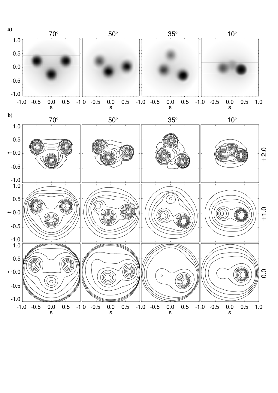
Figure 6: Spatial intensity distribution for a static spherically symmetric model configuration with $\tau=10$ and three source regions for different viewing angles: a) Frequency integrated intensity distribution. b) Intensity distribution for specific frequencies. The frequency is given in Doppler units relative to the line center $(\nu-\nu_{0})/\Delta\nu_{\rm D}$ at the right hand side.

Figure 7: Results obtained for a spherically symmetric model configuration with $\tau=10$ and three source regions for the static case and two different velocity fields (inflow and rotation): a) Emergent line profiles for different viewing angles. b) Two-dimensional spectra for a nearly face-on view (70^∘) and a nearly edge-on view (10^∘). The position and width of the slit is indicated in Fig. 6a. The contours are given for 2.5%, 5%, 7.5%, 10%, 20%, …, 90% of the maximum value.

As a first step towards a full three-dimensional problem without any symmetries, we investigated an axially symmetric, disk-like model configuration ($a:b:c=3:3:1$) with a single source located at ${\bf x}=0$ for several $\tau=\tau({\bf n}_{\rm thick})$ and for different velocity fields. The most optical thick direction ${\bf n}_{\rm thick}$ is the direction within the equatorial plane of the disk. The direction perpendicular to the equatorial plane is the $z$-axis which we also call rotational axis even for cases without rotation.

By means of the static case we show which kind of information can be obtained from the results of our FE code. The emergent line profiles provide global information on the underlying system. They are displayed in Fig. 2a for different optical depths and viewing angles. The viewing angle is defined as the angle between the rotational axis and the direction towards the observer. For instance, a viewing angle of 90^∘ means, the disk is “observed” edge-on. Again, we obtain the characteristical double-peaked line profile for $\tau\ga 1$. The optical thickness decreases for smaller viewing angles. For a viewing angle of $0^{\circ}$ the effective optical depth is only $\tau({\bf n}_{\rm thick})/3$. Consequently, the distance of the peaks in the line profile and the depth of the absorption feature is growing with increasing viewing angle. Note, that the total relative flux $F({\bf n}=0^{\circ})/F({\bf n}=90^{\circ})$ escaping along the $z$-axis is increasing with increasing $\tau({\bf n}_{\rm thick})$. Fig. 2b will be explained later.

Far more information is contained in the spatial distribution of the line intensity projected into the $s$-$t$-plane which is the plane perpendicular to the viewing direction. In Fig. 3a the frequency-integrated intensity distribution is shown for $\tau=10$ and different viewing angles. At 90^∘ the Ly$\alpha$ image shows an elliptical emission line region. The diffuse halo of scattered radiation is most clearly visible. With decreasing viewing angle the diffuse halo becomes less pronounced. For a nearly face-on view (20^∘), the halo is optically thinner and the intensity distribution appears spherically symmetric.

Fig. 3b displays the spatial distribution of the Ly$\alpha$ intensity for different viewing angles (columns) at selected frequencies (rows). For the edge-on view, the intensity distribution strongly depends on the frequency. In the outer line wings at $(\nu-\nu_{0})/\Delta\nu_{D}=\pm 2$ the contours are elliptical and reproduce the disk-like form of the source region. The peaks of the line profile are at $(\nu-\nu_{0})/\Delta\nu_{D}\sim\pm 1$. Here, the major axis of the elliptical intensity distribution in the inner parts of the model is parallel to the rotational axis, whereas the major axis of the elliptical contour lines in the outer parts remains parallel to the equatorial plane of the disk. In the very center of the line ($(\nu-\nu_{0})/\Delta\nu_{D}=0$), the direct view to the source region is blocked by optically thick material. There appear two knots of Ly$\alpha$ emission directly above and below the disk, which are surrounded by an extended elliptical halo. The Ly$\alpha$ knot below the disk vanishes with decreasing viewing angle. At 20^∘ the intensity distribution is spherically symmetric for all frequencies. The observable emission region is most extended at the frequency of the line center.

Two-dimensional spectra from high-resolution spectroscopy provide frequency-dependent data for only one spatial direction. To be able to compare our results with these observations we calculated two-dimensional spectra using the data within the slits indicated in Fig. 3a for the edge-on and nearly face-on view. The results are shown in Fig. 2b for different optical depths. We find that the form of the two-dimensional spectra is relatively insensible to the width of the slit. For $\tau=1$ a single emission region is visible. But already at 90^∘, the highest contour lines reproduce the faint absorption trough of the corresponding line profile (Fig. 2a). The higher the optical depth the wider the gap and the spatial extent of the two peaks. Note that the spatial extent of the outer contour line only depends on $\tau({\bf n}_{\rm thick})$ and not on the viewing direction.

What changes when imposing a macroscopic velocity field is shown in the following two figures. First, we consider an infalling velocity field with $l=0.5$ suitable for a gravitational collapse. Fig. 4a displays the calculated line profiles for different $\tau$ and viewing angles. As expected, the blue peak of the line is enhanced. The higher $\tau$ the stronger the blue peak. Fig. 4b shows the corresponding two-dimensional spectra obtained with the same slit width and position as in the static case. For low optical depth, the shape of the contour lines is a triangle. Photons changing frequency in order to escape via the blue wing are also scattered in space. The consequence is the greater spatial extent of the blue wing. Apart from a growing gap between the two peaks with higher optical depth, the general triangular shape in conserved.

Next, we investigated the elliptical model configuration with Keplerian rotation ($l=0.5$), where the $z$-axis is the axis of rotation. The results are plotted in Fig. 5 for $\tau=1$ and $\tau=10$. The emergent line profiles are symmetric with respect to the line center and show the same behavior with growing optical depth as in the static case. However, the extension of the line wings towards higher and lower frequencies is strongly increasing with increasing viewing angle because of the growing effect of the velocity field. Rotation is clearly visible in the two-dimensional spectra (Fig. 5b). The shear of the contour lines is the characteristical pattern indicating rotational motion. For an edge-on view at $\tau=10$, Keplerian rotation produces two banana-shaped emission regions.

In spite of the relatively low optical depth of the simple model configurations, our results reflect the form of line profiles and the patterns in two-dimensional spectra of many high redshift galaxies. For example, the two-dimensional spectra of the Ly$\alpha$ blobs discovered by Steidel et al. (steidel:etal2000 (2000), Fig. 8) are comparable to the results obtained for infalling (Fig. 4b) and rotating (Fig. 5b) halos. In the sample of van Ojik et al. (vanojik:etal97 (1997)) are many high redshift radio galaxies with single-peaked and double-peaked Ly$\alpha$ profiles. The corresponding two-dimensional spectra show asymmetrical emission regions which are more or less extended in space. De Breuck et al. (debreuck:etal2000 (2000)) find in their statistical study of emission lines from high redshift radio galaxies that the triangular shape of the Ly$\alpha$ emission is a characteristical pattern in the two-dimensional spectra of high redshift radio galaxies. Since the emission of the blue peak of the line profile is predominately less pronounced, most of the associated halos should be in the state of expansion.

6.2 Multiple Sources

High redshift radio galaxies are found in the center of proto clusters. In such an environment, it could be possible that the Ly$\alpha$ emission of several galaxies is scattered in a common halo. To investigate this scenario, we started with a spherically symmetric distribution for the extinction coefficient and with three source regions located at $x_{1}=[0.5,0.25,0]$, $x_{2}=[-0.5,0.25,0]$ and $x_{3}=[0,-0.25,0]$ forming a triangle in the $x$-$y$-plane. In the following figures, the results for $\tau=10$ are presented.

We begin with the static model. Figure 6a shows Ly$\alpha$ images for four selected viewing directions. The specified angle is the angle between the viewing direction and the $x$-$y$-plane. Note that the orientation of the source positions within the plane is different for each image. Viewing the configuration almost perpendicular to the $x$-$y$-plane (70^∘), renders all three source regions visible, because the source regions are situated in the more optically thin, outer parts of the halo. Remember that most of the scattering matter is in and around the center of the system. For other angles, some of the source regions are located behind the center and therefore less visible on the images. Figure 6b shows images at different frequencies. In the line wings at $(\nu-\nu_{0})/\Delta\nu_{D}=\pm 2$, the number and position of the source regions can be determined for all viewing angles. However, at frequencies around the line center at $(\nu-\nu_{0})/\Delta\nu_{D}=\pm 1\;\mbox{and}\;0$, the number of visible sources depends on the viewing angle. Some of the images show only one, other two or three sources.

The corresponding line profiles and two-dimensional spectra are displayed in Fig. 7 for the static case as well as for a halo with global inflow and Keplerian rotation. Width and position of the slits are depicted in Fig. 6a. We get double-peaked line profiles for almost all cases, except for the rotating halo, where the line profiles are very broad for viewing angles lower than 70^∘. Additional features, dips or shoulders, are visible in the red or blue wing. They arise because the three sources have significantly different velocities components with respect to the observer.

The slit for a viewing angle of 70^∘ contains two sources. They show up as four emission regions in the two-dimensional spectra (Fig. 7b). The pattern is very symmetric, even for the moving halos. For a viewing angle of 10^∘, the slit covers all source regions. Nevertheless, the two-dimensional spectra are dominated by two pairs of emission regions resulting from the sources located closer to the observer. The third source region only shows up as a faint emission in the blue part in the case of global inflow. In the case of rotation, emission regions from a third source are present. But the overall pattern is very irregular and prevents a clear identification of the emission regions.

This example demonstrates the complexity of three dimensional problems. In a clumpy medium, the determination of the number and position of Ly$\alpha$ sources would be difficult by means of frequency integrated images alone. Two-dimensional spectra may help, but could prove to be too complicated. More promising are images obtained from different parts of the line profile or information from other emission lines of OIII or H$\alpha$ in a manner proposed by Kurk et al. (kurk:etal2001 (2001)).

7 Summary

We presented a finite element code for solving the resonance line transfer problem in moving media. Non-relativistic velocity fields and complete redistribution are considered. The code is applicable to any three-dimensional model configuration with optical depths up to $10^{3-4}$.

We showed applications to the hydrogen Ly$\alpha$ line of slightly optically thick model configurations ($\tau\leq 10^{2}$) and discussed the resulting line profiles, Ly$\alpha$ images and two-dimensional spectra. The systematic approach from very simple to more complex models gave the following results:

• An optical depth of $\tau\ga 1$ leads to the characteristic double peaked line profile with a central absorption trough as expected from analytical studies (e.g. Neufeld neufeld90 (1990)). This form of the profile is the result of scattering in space and frequency. Photons escape via the line wings where the optical depth is much lower.

• Global velocity fields destroy the symmetry of the line profile. Generally, the blue peak of the profile is enhanced for models with infall motion and the red peak for models with outflow motion. But there are certain velocity fields (e.g. with steep gradients) and spatial distributions of the extinction coefficient, where the formation of a prominent peak is suppressed.

• Double-peaked line-profiles show up as two emission regions in the two-dimensional spectra. Global infall or outflow leads to an overall triangular shape of the emission. Rotation produces a shear pattern resulting in banana-shaped emission regions for optical depths $\ga 10$.

• For non-symmetrical model configurations, the optical depth varies with the line of sight. Thus, the total flux, the depth of the absorption trough and the pattern in the two-dimensional spectra strongly depend on the viewing direction.

The applications demonstrate the capacity of the finite element code and show that the three-dimensional structure and the kinematics of the model configurations are very important. Thus, beside exploring higher optical depths up to the limits of our code, we will consider clumpy density distributions as well as dust absorption and try to model the Ly$\alpha$ emission of individual high redshift galaxies. In addition, we intend to implement a second order method for the frequency discretization. Furthermore, we plan to overcome the difficulties in solving the line transfer problem for configurations with $\tau>10^{4}$. Therefore, we will extend our method and use the diffusion approximation in the most optically thick regions. In the other regions, the full frequency-dependent line transfer problem must be solved.

- (1) Adams, T.F. 1972, ApJ 174, 439
- (2) Ahn, S.-H., Lee, H.-W., & Lee, H. M. 2001, ApJ 554, 604
- (3) Ahn, S.-H., Lee, H.-W., & Lee, H. M. 2002, ApJ 567, 992
- (4) Baschek, B., & Wehrse, R. 1999, Physics Reports 311, 201
- (5) Bicknell, G.V., Sutherland, R.S., van Breugel, W.J.M., et al. 2000 ApJ 540, 678
- (6) De Breuck, C., Röttgering, H., Miley, G., van Breugel, W., & Best, P. 2000, A&A 362, 519
- (7) Fynbo, J.U., Thomsen, B., & Møller, P. 2000, A&A 353, 457
- (8) Fynbo, J.U., Møller, P., & Thomsen, B. 2001, A&A 374, 443
- (9) Hippelein, H., & Meisenheimer, K. 1993, Nature 362, 224
- (10) Hu, E.M., Cowie, L.L., & McMahon, R.G. 1998, ApJ 502, L99
- (11) Hummer, D.G., & Kunasz, P.B. 1980, ApJ 236, 609
- (12) Kanschat, G. 1996, Ph.D. Thesis, Univ. of Heidelberg
- (13) Kurk, J.D., Röttgering, H.J.A., Miley, G.K., & Pentericci, L. 2001, RevMexAA (Serie de Conferencias), in press
- (14) Kudritzki, R.-P., Mendez, R.H., Feldmeier, J.J., et al. 2000, ApJ 536, 19
- (15) Mihalas, D., & Weibel-Mihalas, B. 1984, Foundation of Radiation Hydrodynamics, Oxford University Press, New York
- (16) Neufeld, D.A. 1990, ApJ 350,216
- (17) Richling, S., Meinköhn, E., Kryzhevoi, N., & Kanschat, G. 2001, A&A 380, 776 (Paper I)
- (18) Rhoads, J.E., Malhotra, S., & Dey, A. 2000, ApJ 545, L85
- (19) Steidel, C.C., Adelberger, K.L., Sharply, A.E., et al. 2000, ApJ 532, 170
- (20) van Ojik, R., Röttgering, H.J.A., Carilli, C.L., et al. 1996, A&A 313, 25
- (21) van Ojik, R., Röttgering, H.J.A., Miley, G.K., & Hunstead, R.W. 1997, A&A 317, 358
- (22) Villar-Martín, M., Binette, L., & Fosbury, R.A.E. 1999, A&A 346, 7
- (23) Wehrse R., Baschek B., & von Waldenfels, W. 2000, A&A 359, 780