K dwarfs and the chemical evolution of the Solar cylinder

Abstract

K-dwarfs have life-times older than the present age of the Galactic disc, and are thus ideal stars to investigate the disc’s chemical evolution. We have developed several photometric metallicity indicators for K dwarfs, based an a sample of accurate spectroscopic metallicities for 34 disc and halo G and K dwarfs. The photometric metallicities lead us to develop a metallicity index for K dwarfs based only on their position in the colour absolute-magnitude diagram. Metallicities have been determined for 431 single K dwarfs drawn from the Hipparcos catalog, selecting the stars by absolute magnitude and removing multiple systems. The sample is essentially a complete reckoning of the metal content in nearby K dwarfs. We use stellar isochrones to mark the stars by mass, and select a subset of 220 of the stars which is complete in a narrow mass interval. We fit the data with a model of the chemical evolution of the Solar cylinder. We find that only a modest cosmic scatter is required to fit our age metallicity relation. The model assumes two main infall episodes for the formation of the halo-thick disc and thin disc respectively. The new data confirms that the solar neighbourhood formed on a long timescale of order 7 Gyr.

1 Introduction

A central issue in studies of the chemical evolution of the Galactic disc is to resolve the so called “G-dwarf problem” (van den Bergh, 1962; Schmidt, 1963; Pagel and Patchett, 1975). The problem is that the observed stellar metallicity distribution shows far fewer metal deficient stars than the predictions of the simplest, closed box models of the Galactic disc’s chemical evolution. Integrated light studies indicate that the G-dwarf problem is not restricted to our own disc (Worthey et al, 1996) but is also found in other galaxies. There are many ways that the evolutionary models can be modified to bring them into consistency with the observations, such as pre-enrichment of the gas, a time dependent Initial Mass Function or gas infall (for a review see e.g. Pagel, 1997)

G-dwarfs are sufficiently massive that some of them have begun to evolve away from the main sequence, and these evolutionary corrections must be taken into account when determining their space densities and metallicities. While these problems are by no means intractable, it has been long recognized that K dwarfs would make for a cleaner sample of the local metal abundance distribution, because for these stars the evolutionary corrections are negligible.

K dwarfs are of course intrinsically fainter, and it has not been until recently that accurate spectroscopic K dwarf abundance analyses have become available, with which to calibrate photometric abundance indicators (Flynn and Morell, 1997). As a result, it is now known that there is a K-dwarf problem which is very similar to the G-dwarf problem (Flynn and Morell, 1997). Studies of M dwarfs indicate that the problem is present in these stars too (Mould 1976). Such stars are still not really ideal for measuring the local metallicity distribution, because metallicities for M dwarfs are difficult to determine in the optical (but appears possible using infrared $JHK$ photometry, (see e.g. Stauffer and Hartmann, 1986; Leggett et al, 2000). The all sky surveys presently underway in the infrared (Denis, 2MASS) may make such stars viable metallicity tracers in the near future.

The G-dwarf metallicity distribution is already an extensively studied subject (Pagel and Patchett, 1975; Sommer-Larsen, 1991; Wyse and Gilmore, 1995; Rocha-Pinto and Maciel, 1996) and has been used by chemical evolution models to constrain the time scale of the formation of the Galactic disc at the solar neighbourhood. The G-dwarf metallicity distribution can be well fit by models in which gas has been settling onto the disc over a protracted period, of some billion years. For example, Chiappini et al (1997), on the basis of the fit of the G-dwarf metallicity distribution, have shown that the disc in the solar neighbourhood was formed on a long time scale of 7 - 8 Gyr. This conclusion has been later stressed also by other authors (e.g. Portinari et al, 1998; Prantzos and Silk, 1998; Chang et al, 1999).

The release of the data from the European Space Agency’s Hipparcos (ESA, 1997) satellite offers a great opportunity to determine the local metallicity distribution of the disc from a complete sample of K dwarfs. There are three clear improvements because of Hipparcos. Firstly, the parallaxes are so accurate that the K dwarfs can be selected by absolute magnitude rather than colour, which is a much better way of isolating stars in a particular mass range. Secondly, the uniformity of the Hipparcos data allows us to construct samples with well understood completeness limits. Thirdly, a large fraction of the close binaries can be identified using Hipparcos and removed (since photometric abundance indicators are calibrated for single stars). This last effect turns out to be quite important.

In this paper we develop a number of simple photometric metallicity indicators for K dwarfs, based on a spectroscopically determined sample of metallicities by Flynn and Morell (1997). The metallicities for several hundred K dwarfs drawn from the Hipparcos catalog have been measured via new observations described here. This sample has been used to show that there is a very simple relation between the $V$ band luminosity $M_{V}$ of K dwarfs at a given $B-V$ colour and metallicity (the work is fully described in a companion paper (Kotoneva, Flynn and Jimenez, 2002, paper II). This simple relation is used in this paper to determine metallicities for 431 single K dwarfs in a near complete sample selected from the Hipparcos catalog. We examine a set of isochrones and find a simple relation between the position of a star in the Hipparcos colour magnitude diagram and mass. We are thus able to select a sample of dwarf stars by the more physically relevant parameter of mass, rather than by colour or absolute magnitude, as is usually the case. The metallicity distribution obtained is then compared to the results of models of the chemical evolution of the Solar neighbourhood.

The paper is organized as follows: In section 2 we describe the selection of the K dwarf sample and in section 3 the observations and reductions of the stars in broadband and intermediate band photometric systems. The details of the various metallicity calibrations are presented in section 4. In section 5 we use isochrones to fit the masses of the stars, and select the stars in an appropriate mass range which is near complete; we discuss the kinematics of the stars and compute corrections for the metallicity distribution function from the solar volume to the solar cylinder. The metallicity distribution is compared briefly with other determinations in the literature. We compare the data to the predictions of a model of the chemical evolution of the Solar neighbourhood due to Chiappini et al (2001) in section 6. We draw our conclusions and summarize in section 7.

2 The Sample

2.1 Sample selection

Our sample of K dwarfs is drawn from the ESA Hipparcos catalog (ESA, 1997). For the purposes of this paper we term K dwarfs to be stars of absolute magnitude $M_{V}$ in the range $5.5<M_{V}<7.3$. The choice of these absolute magnitude limits is motivated as follows. The upper magnitude limit at $M_{V}=5.5$ is chosen to avoid the effects of stellar evolution. Examination of theoretical isochrones (see e.g. Jimenez, Flynn and Kotoneva, 1998) indicate that the effects of stellar evolution on luminosity at $M_{V}=5.5$ during the disc lifetime amount to at most $0.1$ magnitude, typically much smaller. The effects of stellar evolution in constructing the sample are thus small, and negligible compared to the main source of error (which is Poisson sampling statistics). The limit at $M_{V}=5.5$ corresponds to a spectral type of about G8. The lower absolute magnitude limit at $M_{V}=7.3$ is the magnitude of the reddest K dwarfs for which our photometric metallicity indicators can currently be calibrated via spectroscopic observations (Flynn and Morell, 1997). The limit at $M_{V}=7.3$ corresponds a spectral type of about K5.

Since we are interested in obtaining a complete sample of K dwarfs in the Solar neighbourhood, with which to construct the metallicity distribution function (MDF), the stars were initially selected from the “survey” part of the Hipparcos catalog, which is complete to an apparent visual magnitude given by $V<7.3+1.1\,{\mathrm{s}in}|b|$. Here $b$ is the Galactic latitude (the apparent visual magnitude limit was made dependent on $b$ in order to avoid observing excessive numbers of stars in the Galactic plane). Adopting this apparent magnitude limit and the absolute magnitude range $5.5<M_{V}<7.3$ resulted in a sample of 209 stars. Our intention had been to get a sample of order 500-750 stars. In order to increase our basic sample size, we increased the magnitude limit by 0.9 mag (i.e. by taking an apparent magnitude limit of $V<7.3+1.1\,{\mathrm{s}in}|b|+0.9$) we obtained 668 stars (including the first 209 stars). This is the basic sample which we targeted for observations.

We need to understand the completeness of this basic sample, since it is drawn from stars 0.9 magnitudes fainter than the magnitude limit of the complete part of the Hipparcos catalog. Even 0.9 magnitudes beyond the completeness limit, the sample turns out to be still satisfactorily close to complete for our purposes. The completeness level is approximately 94%. We determined this quantity by using the Galactic structure model of Holmberg (2000). The model is based on star count data and makes use of both the Hipparcos and Tycho data (the latter is complete to much fainter limits than Hipparcos) to construct the luminosity function of the local disc. Using the model, we find that for an apparent magnitude limit of $V<7.3+1.1\,{\mathrm{s}in}|b|+0.9$ and absolute magnitude limits of $5.5<M_{V}<7.3$, we would expect that some 710 stars should be in our basic sample, whereas there are actually 668 such stars in the Hipparcos catalog. We conclude that even 0.9 magnitudes beyond the “survey” completeness limit, Hipparcos is substantially (94%) complete in the absolute magnitude range of interest.

Stars were observed by Hipparcos up to 4 magnitudes fainter than the faintest stars in the “survey”. The 0.9 magnitude extension beyond the survey limit results in a sample which is still over 90% complete. Beyond this 0.9 mag limit, completeness drops rapidly, and the stars in Hipparcos become increasingly dominated by objects included for a particular astrophysical interest, such as having a low metallicity and/or high velocity. There will be a very small excess of such stars in our extended sample, but the high completeness (94%) means that it is other uncertainties (Poisson statistics) which dominate the construction of the metallicity distribution.

Figure 1: The upper panel shows colour-magnitude diagram for 431 stars in our sample for which $B-V$ colour is available, while the lower panel shows the colour-magnitude diagram for the $R-I$ colour. Note that the main sequence is clearly thicker as a function of $B-V$ compared to $R-I$. This is a direct consequence of the metallicity of the stars, which affects $B-V$ much more than it affects $R-I$ (Flynn and Morell, 1997).

2.2 Removal of multiple stars

The photometric metallicity indicators described in section 4 were calibrated using spectroscopically determined metallicities for single stars. We examined the effect that multiple stars would have on our metallicity indicators, by making Monte-Carlo simulations in which we combined the fluxes of a range of pairings of single K and M dwarfs selected at random from the Hipparcos delineated main sequence, and computing the effect on the photometrically determined metallicity. Metallicities for multiple stars were found to be as much as $0.4$ dex lower than the true metallicity. Cleaning the sample of multiple stars thus turned out to be very important.

The Hipparcos catalog included a flag for “probable multiple stars”, based on the “reliability of the double or multiple star solution”. This flag was used to eliminate all definite, possible and suspected multiple systems. This reduced the sample from 668 to 449 stars or about 2/3 of the initial sample. Despite this expedient, a small number of binaries seem to remain in the sample (of order 10%). This is evident from the positions of the suspected multiples in the colour-magnitude and two colour $B-V$ versus $R-I$ diagrams. This issue is studied in detail in a companion paper (Kotoneva, Flynn and Jimenez, 2002, Paper II). About half of these extra suspected multiples could be removed in constructing the final sample, so the final sample should have a minor contamination by multiples of less than 5%. Note that, by “single stars”, we mean only stars which have no companion bright enough to significantly affect the metallicity measurement (i.e. within 5 magnitudes of the brightness of the primary). After removing these suspected multiple stars the final sample consists of 431 stars.

The colour-magnitude diagrams for our final sample of single stars are shown in Fig 1.

3 Observations and reductions

Observations were made at Siding Spring Observatory (SSO) in Australia, between $8^{\mathrm{t}h}$ and $22^{\mathrm{n}d}$ of March 1999. We measured Johnson-Cousins and Strömgren colours for all available Southern hemisphere stars of the basic sample using the SSO 24” telescope. We used the Motorized Filter Box with all eight filters $U,B,V,R,I$ and Strömgren $v,b$ and $y$. $UBVRI$ primary standards were selected from Landolt (1983a, 1983b, 1992) and among E-region standard stars (Graham, 1982; Menzies et al., 1989). Strömgren primary standards were selected from the E-regions and also from Grønbech, Olsen, and Strömgren (1976) and Crawford and Barnes (1970). Hauck and Mermilliod (1998) stars were used as secondary standards for the Strömgren system and Flynn and Morell (1997) stars for both of the intermediate band systems. We observed 218 stars and 55 of these more than once. The standard error in the $R-I$ colour was $\approx 0.012$ mag, quite accurate enough for our purposes. In the Strömgren bands the photometric error was slightly higher but still $\approx 0.02$ mag.

Further data were obtained at La Palma using the Swedish 60 cm telescope in March 2000. An SBIG CCD was used to observe in the filters $V,R$ and $I$. 90 stars were observed, most of them more than once. The scatter for the La Palma observations was bit higher than at SSO, the scatter in the $R-I$ band being 0.021 for a single observation. Since most of the stars were observed twice the mean error came down to $\approx 0.015$ mag. 22 of the stars were observed both in Australia and La Palma; the mean difference in $R-I$ was less than 0.01 mag and the scatter was 0.01 mag, so that no significant difference was found between observations taken at the different observatories.

We also obtained $R-I$ colours for 108 stars from Bessell (1990), who observed all the stars in the Gliese catalog. These are found to be in excellent agreement with our own SSO data with a mean difference in $R-I$ of less than 0.01 mag with a scatter of 0.013 mag. A comparison of the two sources of $R-I$ colour is shown in Fig 2.

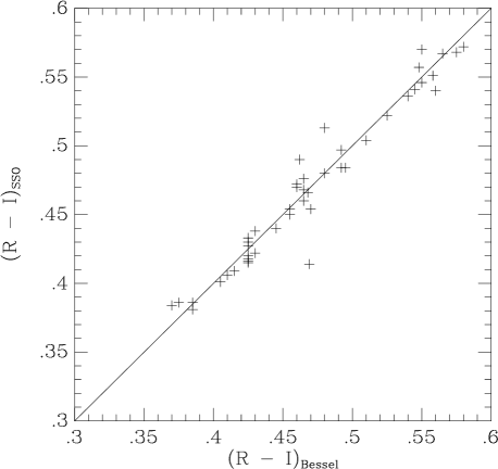
Figure 2: Comparison of our $R-I$ colours obtained at SSO versus those from Bessell’s (1990) values from his observations of stars in the Gliese catalog. The mean difference is less than 0.01 mag and the scatter is 0.013 mag.

4 Determination of Metallicities

We have obtained metallicities for all 431 stars of the dataset. In the end, a single method was used, although we discuss here four metallicity indicators for the dwarfs. Firstly, we used a relation based on Geneva and $R-I$ photometry due to Flynn and Morell (1997). Secondly, we have developed a very similar method to Flynn and Morell’s based on Strömgren and $R-I$ colours. Thirdly, we have found a simple relation between the broadband $B-V$ and $V-I$ colours and metallicity. Fourthly, we have developed in a companion paper (Kotoneva, Flynn and Jimenez, 2002) a metallicity indicator for K dwarfs based on their absolute magnitude in the $V$ band relative to a fiducial solar metallicity isochrone. The first three methods have a similar error 0.2 dex in $[{\rm Fe/H}]$, while the last method appears to be better, with an estimated error of 0.1 dex. This last method depends on the availability of accurate parallaxes for the stars, and so is less generally applicable than those which rely on photmetric colours alone. The last method is the one we adopt here for measuring the K dwarf metallicities.

4.1 Metallicities from Geneva photometry

To obtain the metallicities for the K dwarfs for which a Geneva $b_{1}$ colour is available, we used existing relations described in Flynn and Morell (1997). The $b_{1}$ colours were obtained from Rufener (1989) for 245 stars and the $R-I$ colours come from our observations and/or from Bessell (1990). Both of the colours were available for 149 stars for which the metallicities, [Fe/H]${}_{b_{1}}$, were computed using the relation:

$${\rm[Fe/H]}_{b_{1}}=8.248\times b_{1}-12.822\times(R-I)-4.822.$$ (1)

These metallicities have a typical error of 0.2 dex.

4.2 Metallicities from Strömgren photometry

We have developed a new metallicity indicator for the K dwarfs for which Strömgren colours are available. The calibration was obtained using the 34 G and K dwarfs from Flynn and Morell (1997). For these stars accurate, spectroscopically determined metallicities, [Fe/H]_spec and effective temperatures have been determined with errors of 0.05 dex and $\approx 100$ K, respectively.

We searched for a relation between $R-I$ colour, Strömgren colours and spectroscopical abundance, $[{\rm Fe/H}]_{\mathrm{s}pec}$. The best fitting Strömgren colour was found to be $m_{1}$, with a small dependence on $c_{1}$. The $b-y$ colour was found to be poorly correlated with metallicity as one might expect. The relation we found is:

$${\rm[Fe/H]}_{m_{1}} = 6.076\times{\rm m_{1}}-3.811\times{\rm c_{1}}+9.4303\times{\rm c_{1}}^{2}$$

$$-12.822\times{\rm(R-I)}+3.226.$$

Fig 3 shows the relation between the spectroscopically determined metallicity and the Strömgren and $R-I$ based metallicity. The scatter around the one-to-one relation is $\approx 0.20$ dex.

For 142 stars both the Strömgren $m_{1}$ and $c_{1}$ colours and $R-I$ colour were available and the metallicities $[{\rm Fe/H}]_{m_{1}}$ were calculated. The dependence on $c_{1}$ is quite weak, so that while for 54 stars no $c_{1}$ colour was available, for these stars we adopted a typical value of $c_{1}=0.29$. Adopting this mean value leads to a very small increase in the metallicity error of $\approx$ 0.02 dex.

Figure 3: Relation between the metallicities using Strömgren $m_{1}$ colour and spectroscopically determined metallicities. The scatter around the 1:1 line is $\approx 0.20$ dex.

4.2.1 A check using the Hyades

A check of the Strömgren calibration was made using G and K dwarfs in the Hyades cluster (Reid, 1993; Flynn and Morell, 1997), using $VRI$ photometry and Strömgren $m_{1}$ colour from the literature (Hauck and Mermilliod, 1998). A list of the Hyades G and K dwarfs, their magnitudes, $B-V$, $R-I$ and $m_{1}$ colours and the metallicities calculated using eqn. (2) are shown in Table 1. Taylor (1994) estimated the mean metallicity for the Hyades to be $[{\rm Fe/H}]=0.11\pm 0.01$. Our mean value is $[{\rm Fe/H}]=0.16\pm 0.03$. Fig 4 shows the relation between the derived metallicity and the $R-I$ colour, and is found to be independent of colour, indicating that there are no residual temperature effects in the metallicity indicator.

Table 1: Broadband and Strömgren $m_{1}$ data for G and K dwarfs in the Hyades

HD no.	$V$	$R-I$	$m_{1}$	$[{\rm Fe/H}]_{m_{1}}$
26756	8.46	0.35	0.25	0.01
26767	8.04	0.31	0.21	0.36
27771	9.09	0.39	0.38	0.26
28099	8.10	0.32	0.23	0.01
28258	9.02	0.43	0.36	$-$0.37
28805	8.66	0.35	0.29	0.21
28878	9.38	0.41	0.42	0.20
28977	9.65	0.44	0.45	0.00
29159	9.37	0.41	0.40	0.09
30246	8.31	0.33	0.24	0.18
30505	8.98	0.38	0.37	0.31
32347	8.98	0.36	0.31	0.20
284253	9.14	0.38	0.35	0.20
284787	9.05	0.40	0.37	0.05
285252	9.00	0.41	0.43	0.28
285690	9.56	0.44	0.52	0.43
285742	10.26	0.49	0.59	0.12
285773	8.94	0.41	0.36	$-$0.12
285830	9.47	0.44	0.45	0.06
286789	10.44	0.52	0.70	0.47
286929	10.01	0.51	0.63	0.15

Figure 4: The metallicities $[{\rm Fe/H}]_{m_{1}}$ for Hyades G and K dwarfs as a function of $R-I$. The dotted line represents the mean metallicity value from the literature $[{\rm Fe/H}]=0.11$ (Taylor, 1994). Our mean value $[{\rm Fe/H}]=0.16$ is shown as a solid line.

4.3 Comparison of the Strömgren and Geneva photometric metallicity calibrations

In Fig 5 the relation between the metallicities calculated using the Geneva colour $b_{1}$ and the Strömgren $m_{1}$ colour is shown. The separate metallicities are in good agreement with each other: the scatter around the fitted line is only $0.15$ dex, significantly less than the error of the individual metallicity estimates of 0.2 dex. This is probably because the $b_{1}$ and $m_{1}$ colours are correlated, since they both measure similar regions in the blue at approximately 4000 Å. The metallicities are found to be in excellent agreement for $[{\rm Fe/H}]>-0.7$, where most of the stars lie, differing by less than 0.01 dex. For the stars with metallicities $[{\rm Fe/H}]<-0.7$, the scatter appears to increase and there may be some systematic shift between the systems. In terms of the K dwarf problem, a possible systematic error at such low metallicity is not very significant. More low metallicity stars with good spectroscopic metallicity determinations would be of interest for testing the abundance indicators further.

Figure 5: The relation between the metallicities based on the Strömgren $m_{1}$ and Geneva $b_{1}$ colours. The solid line shows a least square fit to the data (where the errors in both colours are taken into account). The dotted line shows the 1:1 relation.

4.4 Metallicities from broadband photometry

We have also developed a new metallicity indicator for K dwarfs using broadband $BVI$ photometry. For this purpose we only choose calibration K dwarfs in the absolute magnitude range $5.5<M_{V}<7.3$. The calibration stars were selected from the Flynn and Morell (1997) sample, with $B-V$ and $V-I$ data being collated from Bessell (1990). The calibrating sample is shown in Table 2. We recovered a simple relation between $B-V$, $V-I$ colour and metallicity as follows:

$$[\mathrm{F}e/H]_{\mathrm{B}VI}=8.54\times(B-V)-7.73\times(V-I)-0.55$$ (3)

where we denote the metallicity index based on these colours by [Fe/H]_BVI. A comparison of the spectroscopic metallicities and this broadband photometric metallicity indicator is shown in Fig 6. The scatter in the fit is $\approx 0.1$ dex. Note that this simple relation should not be used for stars with absolute magnitude $M_{V}<5.5$, because the effects of stellar evolution begin to affect the colours in addition to the metallicity.

Table 2: K dwarfs used to calibrate a photmetric metallicity indicator based on $B-V$ and $V-I$ colours. Columns are the HD number, colours, absolute magnitude $M_{V}$, the spectroscopically measured metallicity [Fe/H]_spec and the photometric metallicity [Fe/H]_BVI (Eqn. 3)

HD no.	$B-V$	$V-I$	$M_{V}$	[Fe/H]spec	[Fe/H]BVI
4628	0.890	0.949	6.376	$-0.40$	$-0.29$
10700	0.727	0.802	5.680	$-0.50$	$-0.54$
13445	0.812	0.891	5.930	$-0.28$	$-0.50$
25329	0.863	1.093	7.178	$-1.70$	$-1.63$
26965	0.820	0.888	5.916	$-0.30$	$-0.41$
64090	0.621	0.865	6.008	$-1.90$	$-1.93$
72673	0.780	0.853	5.953	$-0.35$	$-0.48$
100623	0.811	0.870	6.063	$-0.25$	$-0.35$
103095	0.754	0.934	6.611	$-1.40$	$-1.33$
134439	0.770	0.959	6.736	$-1.57$	$-1.39$
134440	0.850	1.037	7.077	$-1.52$	$-1.31$
149661	0.827	0.832	5.819	$0.00$	$0.08$
192310	0.878	0.888	6.002	$-0.05$	$0.08$
209100	1.056	1.118	6.893	$-0.10$	$-0.17$
216803	1.094	1.169	7.065	$-0.20$	$-0.24$

The metallicity index is quite accurate, and is based on broadband colours only. As a consequence it is probably more useful than the indices based on the narrower band Strömgren and Geneva colours developed in the previous sections. A simple test of the calibration could be obtained by selecting low reddening open and globular clusters for which sufficiently deep main sequence photometry in $B,V$ and $I$ is available, since metallicities for these are known from spectroscopic studies.

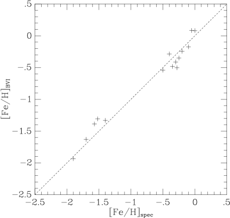
Figure 6: Relation between the metallicities using the broadband colours $B-V$ and $V-I$ for K dwarfs in the absolute magnitude range $5.5<M_{V}<7.3$. The scatter around the 1:1 line is $\approx 0.1$ dex.

By applying this type of metallicity indicator to large photometric surveys (such as Sloan) it would be in principle possible to estimate the metallicity distribution of K dwarfs at different Galactocentric distances in the Milky Way’s disk and even in the bulge region. This would represent an powerful constraint for chemical evolution models. Moreover this metallicity indicator could also be used to study local group galaxies by utilizing deep two color data obtained with Hubble Space Telescope.

4.5 Metallicities using K dwarf luminosity and colour

We show in a companion paper (Kotoneva, Flynn and Jimenez, 2002) that stellar luminosity on the main sequence correlates very well with metallicity at a given colour. This was shown by measuring the displacement of stars $\Delta M_{V}$ of K dwarfs from a fiducial isochrone in the $M_{V}$ versus $B-V$ plane (i.e. relative to the fiducial line at that colour). The fiducial isochrone comes from Jimenez, Flynn and Kotoneva (1998), has an age of 11 Gyr, solar metallicity, and was found empirically to be a good fit to solar metallicity K dwarfs. The metallicity determined by this method, [Fe/H]_KF, is given by:

$${\rm[Fe/H]_{\mathrm{K}F}}=1.185\times\Delta M_{V}+0.054.$$ (4)

This new metallicity indicator was developed on the basis of the photometric derived metallicities described above. When we checked that [Fe/H]_KF is consistent with the sample of K dwarfs with spectroscopically determined metallicities (and in which it is ultimately based, since the photometric metallicities have been calibrated from these same dwarfs) the indicator turned out to be considerably more accurate than anticipated. The scatter between the [Fe/H]_KF and the spectroscopically measured metallicities was $\approx 0.08$ dex, i.e. little more than the intrinsic error in the spectroscopic metallicities (0.05 dex). Although the spectroscopic sample is rather small, we consider that metallicities derived using this technique are greatly superior to photometrically derived metallicities. Note that the technique relies on accurate parallaxes (absolute magnitudes) being available, and is at present applicable only to nearby stars (or stars for which an independent distance indicator is available). Alternatively, the photometric techniques developed in this paper, although of lower precision, can be used on stars for which colours only are available.

For all the stars in the sample we show the metallicity [Fe/H]_KF in column 12 of Table 3. The values are based on the Hipparcos $B-V$ and $M_{V}$. The error in [Fe/H] is dominated by the colour error, which for the sample stars is typically 0.025 mag, leading to a typical error in the metallicities of 0.1 dex.

5 K dwarfs in the Hipparcos catalog

5.1 The data

Part of the full dataset of 431 stars is shown in Table 3. The table shows the Hipparcos Input catalog (HIP) and HD numbers, visual magnitude $V$ and absolute magnitude $M_{V}$, as computed from the Hipparcos parallax. The next five columns are the $B-V$ colour, the mean values of $R-I$ and $m_{1}$ and $c_{1}$ Strömgren colours and $b_{1}$ from the Geneva catalog. The Strömgren based metallicity, ${\rm[Fe/H]}_{m_{1}}$, Geneva based metallicity ${\rm[Fe/H]}_{b_{1}}$ and the luminosity based metallicity ${\rm[Fe/H]}_{KF}$ follow. The three last columns show the $U,V$ and $W$ velocities in km s^-1. The full dataset is available at the Strasbourg Data Center or from the authors.

Table 3: Part of the dataset showing identifications (HIP and HD numbers), visual $V$ magnitude, absolute magnitude $M_{V}$, broadband colours $B-V$ and $R-I$, Strömgren colours $m_{1}$ and $c_{1}$, the Geneva colour $b_{1}$, abundance estimates from various methods (see section 5) and the space velocities $U,V$ and $W$. The full table of 431 stars is available at the Strasbourg Data Center or from the authors.

HIP	HD	$V$	$M_{V}$	$B-V$	$R-I$	$m_{1}$	$c_{1}$	$b_{1}$	$[{\rm Fe/H}]$	$[{\rm Fe/H}]$	$[{\rm Fe/H}]$	$U$	$V$	$W$
									$m_{1}$	$b_{1}$	KF
1031	870	7.22	5.68	0.77	–	0.29	0.28	1.17	–	–	$-$0.27	–	–	–
1085	924	9.05	6.44	0.91	–	0.42	0.28	–	–	–	$-$0.35	–	–	–
1837	1910	8.74	7.01	1.08	–	–	–	1.40	–	–	$-$0.26	–	–	–
1936	2025	7.92	6.64	0.94	0.48	0.47	0.23	1.28	$-0.43$	$-0.39$	$-$0.45	$-$41	$-$7	$-$1
2194	2404	9.02	5.70	0.75	–	0.24	0.26	1.13	–	–	$-$0.44	–	–	–
2736	3167	8.97	5.70	0.83	–	–	–	–	–	–	0.08	–	–	–
2742	3141	8.02	5.71	0.87	–	0.41	0.31	–	–	–	0.29	32	25	0
2743	3222	8.55	6.21	0.85	–	0.37	0.29	1.24	–	–	$-$0.41	$-$64	$-$102	44
3028	3569	9.21	6.11	0.85	–	–	–	–	–	–	$-$0.30	–	–	–
3206	3765	7.36	6.17	0.94	–	0.49	0.30	1.30	–	–	0.10	29	$-$67	$-$20
3535	4256	8.03	6.32	0.98	0.46	–	–	1.35	–	0.42	0.10	42	$-$23	$-$27

5.2 Raw metallicity distribution function for K dwarfs

The normalised metallicity distribution function (MDF) for our basic sample of 431 K dwarfs is shown in the upper panel of Fig 7, and is based on the [Fe/H]_KF metallicities. There are two studies of the metallicity distribution of K dwarfs in the literature with which we can compare our results. We compare the raw MDF, because this most closely matches the procedures which have been used to select K dwarf samples in the past (rather than comparing to the more carefully selected sample of K dwarfs described in the next section).

Fig 7 also shows the metallicity distribution functions obtained by Marsakov and Shevelev (1988) and Rocha-Pinto and Maciel (1998b, RPM98). The Marsakov and Shevelev sample is an inhomogeneous compilation of metallicities from the literature. The Rocha-Pinto and Maciel stars were selected from the Third Gliese catalogue (Gliese et al, 1991), for which photometric data could be found from the literature. The present sample is a near complete sample of the solar neighbourhood based on Hipparcos parallaxes and new photometric observations. The samples have rather different pedigrees, but they are all similar to the metallicity distribution for G dwarfs, being peaked at $\simeq-0.2$ dex.

The clear result in Fig 7 is that the metallicity distribution we obtain here is broader than the other samples. We believe this can be attributed to the selection of our sample by absolute magnitude rather than by spectral type. We will argue this view in section 5.6, and use what we regard as a superior procedure of selecting the stars by mass, rather than spectral type, colour or luminosity, as has been done in the past.

Figure 7: Normalised metallicity distribution functions (MDF) for K dwarf sampes in the literature and for this study. Lower panel : Rocha-Pinto and Maciel (1998b). Middle panel: Marsakov and Shevelev (1988). Upper panel: the 431 stars in our basic sample, before any corrections. The three samples all show a similar spread in abundance and a peak at $[{\rm Fe/H}]\approx-0.2$. The present sample (upper panel) clearly shows a longer tail of super-solar metallicity stars; this is a consequence of the selection of the stars by absolute magnitude. In section 5.6 we develop a selection by stellar mass which substantially reduces the number of stars at super-solar metallicities.

Haywood (2001) has shown that the metallicity distribution of nearby G dwarfs for all samples in the literature peak at ${\rm[Fe/H]}\approx-0.2$, as does the present K-dwarf sample and the RPM98 sample. Haywood (2001) however argues that the peak should be at ${\rm[Fe/H]}=0.0$, based on samples selected by colour and not spectral type, as has been done in the past. Our sample is selected by absolute magnitude rather than colour, since this more reliably selects the stars by mass, yet we still find the peak at its traditional location. A comparison of 101 stars in common between Haywood’s and our sample does, indeed, show an offset between our stars and his of 0.2 dex. Furthermore, a comparison with 40 stars in common with Rocha-Pinto and Maciel (1998b) shows an offset of 0.15 dex (in the same sense as the Haywood comparison). These two comparisons are not independent because the metallicities derived for the stars are partially based on Strömgren photometry in both cases. Closer comparison with the Haywood sample shows that the offset is a linear function of the absolute magnitude of the stars, rising from $\approx 0.0$ at $M_{V}=5.5$ to $\approx 0.4$ at $M_{V}=7.3$. Fig 8 shows the Haywood stars (the “long-lived dwarfs”) in $B-V$ colour versus [Fe/H]. The super-solar metallicity stars dominate preferentially among the cooler dwarfs, which suggests that there may be a systematic error in the metallicities as a function of colour (i.e. effective temperature) or some selection effect. Subsequent to noting this trend, we found that it has already been commented upon by Reid (2002). We note that restricting the Haywood sample to $B-V<0.7$ would put the peak in the metallicity distribution at its traditional location (as we find here) at ${\rm[Fe/H]}\approx-0.2$. We will later select our K dwarf sample by mass (section 5.6). The metallicity distribution is not significantly altered if we divide the K dwarfs into subsamples by mass (see Fig 13) within our adopted mass limits.

Figure 8: Colour versus metallicity for the Haywood (2001) sample of long-lived dwarfs. There is a systematic change on the metallicity distribution with stellar colour, with the super-solar metallicity stars dominating amongst the cooler spectral types.

5.3 K dwarf kinematics

The basic sample consists of 431 K dwarf stars with metallicity estimates accurate to $\approx 0.1$ dex. For 212 of the stars, radial velocities were found in the literature and space velocities $U$, $V$ and $W$ computed. Unfortunately, velocities are not available for all the stars; thus there is likely to be a small bias toward higher velocity stars in the literature sources, since high proper motion and metal weak stars are preferentially included in radial velocity programs. However, since about half the sample does have radial velocities, and the sample is furthermore dominated by thick disc and disc stars which have much smaller proper motions than halo stars, the bias in the measured velocity dispersions is likely to be quite small. A useful extension to this work would be to obtain velocities for all the stars.

The velocities are shown as a function of metallicity in Fig 9. The velocity dispersions $\sigma_{U},\sigma_{V}$ and $\sigma_{W}$ are shown as a function of metallicity in Fig 10. The figures show the expected features of the solar neighbourhood: the thin disc with vertical velocity dispersion of about 20 km s^-1for metallicities above approximately [Fe/H] $=-0.5$, the kinematically hotter thick disc in the range $-1\la$ [Fe/H] $\la-0.5$. There are very few stars with halo-like kinematics (high velocity dispersion and high asymmetric drift). This is as one would expect: for a local sample consisting initially of 431 K dwarfs, one would only expect of order 1 halo star, since the local disc:halo normalization is approximately 500:1 (Gould, Flynn and Bahcall, 1998). The apparent low metallicity stars are more likely the result of scatter from stars in the thick disc, since there is an observational scatter in the metallicities of 0.1 dex.

Figure 9: Space motions $U$, $V$ and $W$ of the K-dwarfs as a function of the metallicity [Fe/H]_KF. Note that the velocity scale is different in each panel.

Figure 10: Velocity dispersions $\sigma_{U}$, $\sigma_{V}$ and $\sigma_{W}$ of the K dwarfs versus the metallicity [Fe/H]_KF. The vertical velocity dispersion $\sigma_{W}$ has been fit linearly with metallicity (upper panel) and is used to correct the raw metallicity distribution function for the effect of the scale heights of the stars.

5.4 Scale height/velocity correction

Models of the chemical evolution of the local disc predict the metallicity distribution in a column through the disc, whereas the sample K dwarfs are drawn from a roughly spherical region centered on the Sun. The local sample is therefore biased toward stars of lower velocity dispersion since they will spend more time close to the Galactic mid-plane than older, faster moving stars.

We correct for this by computing the velocity dispersion of the stars as a function of metallicity, and computing from this their vertical scale height using a realistic mass model of the Galactic disc (following Sommer-Larsen, 1991).

Table 4: Scale height correction for the metallicity distribution. The first column shows the metallicity ranges of the bins, the second column shows the observed velocity dispersion of the stars in the bin, $\sigma_{W}$(obs), the third column the fitted vertical velocity dispersion, $\sigma_{W}$(fit) (i.e. to the linear relation shown in the upper panel of Fig 10). The final column shows the ratio $f$ of the column density to the local density of the K dwarfs computed in a model of the Galactic disc (normalised so that $f=1.0$ at [Fe/H] $=-0.02$). The total mass density of the K dwarfs in the model is 0.0043 ${~{}{\rm M}_{\odot}}pc^{-3}$ and the total column density ($|z|<2000.0$ pc) is 3.5 ${~{}{\rm M}_{\odot}}pc^{-2}$.

[Fe/H]	$\sigma_{W}$(obs)	$\sigma_{W}$(fit)	$f$
	${\rm kms^{-1}}$	${\rm kms^{-1}}$
$-0.80$	21.9	23.1	1.99
$-0.50$	25.2	20.5	1.57
$-0.39$	15.9	19.6	1.43
$-0.30$	21.8	18.8	1.32
$-0.23$	22.3	18.2	1.23
$-0.17$	11.8	17.7	1.16
$-0.09$	15.1	17.0	1.07
$-0.02$	16.6	16.4	1.00
$0.09$	14.6	15.4	0.89
$0.25$	14.8	14.0	0.74
$0.52$	12.6	11.7	0.51

The vertical velocity dispersions are tabulated in Table 4 and shown in the upper panel of Fig 10. In order to smooth out noise due to the small sample size, we have fit the vertical velocity dispersion linearly as a function of metallicity (shown as a solid line in the upper panel of Fig 10. We use the fit values of the velocity dispersion in what follows to determine the correction of the MDF for the scale height of the stars.

The volume density of matter in main sequence dwarfs in the absolute magnitude range $5<M_{V}<8$ is 0.0074 ${\rm M}_{\odot}$ pc^-3 (Holmberg and Flynn, 2000, Table 1). The part of this which is represented by our sample K dwarfs ($5.5<M_{V}<7.3$) is 0.0043 ${\rm M}_{\odot}$ pc^-3 (Holmberg, 2001, private communication). We have determined the vertical velocity dispersion for the K dwarfs as a function of metallicity, by sorting the stars by metallicity and dividing them into 11 equal star number bins (so that each bin represents a local volume density of $0.0043/11=0.00039$ ${\rm M}_{\odot}$ pc^-3). From this local density and the velocity dispersion of each bin, we then compute the total column density represented by each bin by integrating self-consistently the Poisson-Boltzmann equations in a model of the local Galactic disc (Holmberg and Flynn, 2000). A correction factor $f$, which is the ratio of the column density to the local density for each bin, normalised so that $f=1$ in the bin closest to the solar abundance (i.e. at [Fe/H] $=-0.02$), is computed and is shown in Table 4.

5.5 Chromospheric activity corrections

In this section we investigate the effects on the metallicity distribution of G or K dwarfs of chromospheric activity.

Due to the Wilson-Bappu effect (Wilson and Bappu, 1957; Wilson, 1976), photometrically derived metallicities differ somewhat from spectroscopic ones (RPM98, Rocha-Pinto and Maciel 1998a and references therein). The Wilson-Bappu effect in active chromospheres causes an emission line in the center of the stellar absorption lines, which leads to too low photometrically determined [Fe/H] metallicities. If a sample includes many active stars, the metallicity distribution would be biased towards metal poor stars.

The effect on the present sample turns out to be quite small. Firstly, chromospheric activity is stronger among binary stars. In the present sample the binaries have been very effectively removed due to the high quality Hipparcos data for all the stars. The sample is therefore similar to RPM98, in which the binaries were also removed. Following RPM98, we can expect that about 30% of the stars the sample are chromosphericaly active after removing the binaries. The metallicity of these stars will be systematically incorrect.

RPM98 have defined a correction to the metallicity distribution, for metallicities determined by Strömgren photometry, for G and K dwarfs. A similar analysis as in RPM98 has been carried out for Geneva photometry (a medium band filter system quite similar to the Strömgren system), using those stars in our sample for which accurate spectroscopic metallicities and measurements of the emission line width $R_{HK}$ are available (Rocha-Pinto, private communication). Although this yielded only 8 stars, the same trend was found for Geneva based metallicities as was found by RPM98 for Strömgren based metallicities. Detailed computations show that the effect of this correction is to shift the mean of the metallicity histogram by $\approx+0.05$ dex, which can be easily understood since $\approx 30$% of the stars are thought to be chromospherically active and the mean correction to ${\rm[Fe/H]}$ for such stars is 0.15 dex (RPM98, their section 4).

In the final sample of K dwarfs, we used metallicities based on the position of the stars in the Hipparcos colour magnitude ($B-V$ versus $M_{V}$) diagram, rather than the purely colour based (intermediate band) metallicities above. Campbell (1984) has shown that the $B-V$ colours of lower main sequence stars in the Hyades are affected by stellar activity, with typical changes in the $B-V$ colour of order $\pm 0.02$ mag; this would change the measured metallicities for the active stars by approximately $\pm 0.1$ dex. Unfortunately, without a detailed study, we cannot be sure if the effect would also yield a systematic error in the metallicities.

In light of the above, we have decided not to make a chromospheric activity correction to the sample because we cannot quantify its effect well enough. The correction is likely to be small ($\approx 0.05$ dex), and probably shifts the position of the peak of the metallicity distribution rather than changing its shape. A major result of the paper, that the K dwarfs have a similar metallicity distribution to the G dwarfs, is therefore robust despite the uncertainties surrounding what chromospheric corrections should be applied, if any.

5.6 K dwarf masses

In the past, the metallicity distribution function (MDF) of the local disc has been determined for stars of a particular spectral type or in some colour range. However, in the context of modelling the chemical evolution of the Galaxy and fitting it to the observed MDF, it is the range of stellar masses represented in the MDF which is of most interest. Selection of the stars within a particular range of masses permits a more direct comparison between the observations and theory. We describe in this section the use of isochrones to estimate masses for the K dwarfs.

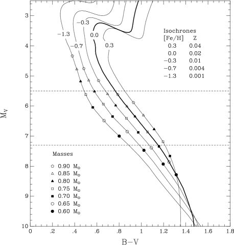
Figure 11: Yonsei-Yale (Y²) isochrones for a range of metallicities. The positions of stars of various mass are marked with different symbols. In the K dwarf region, $5.5<M_{V}<7.3$ (dashed horizontal lines) there is a simple relation between mass, absolute magnitude $M_{V}$ and colour $B-V$.

We show in Fig 11 the 5 Gyr Yonsei-Yale (hereafter Y²) isochrones (Yi et al, 2001) for a range of metallicities. Also marked are the positions on each isochrone at which stars of masses 0.90, 0.85, …, 0.60 M_⊙ lie. The two horizontal lines indicate the absolute magnitude cuts which were used to construct the basic sample, $5.5<M_{V}<7.3$. Within the absolute magnitude range of interest, there is clearly a simple relation between mass and position in the colour-magnitude diagram. We have fit the mass $M$ (in M_⊙) as a function of $M_{V}$ and $B-V$ as follows

$$M=0.322\times(B-V)-0.169\times M_{V}+1.551.$$ (5)

The relation was found by fitting mass, colour and luminosity in the Y² isochrones for ages ranging between 2 and 10 Gyr. The internal precision in the relation is quite good, with a scatter of 0.03 M_⊙ in the mass determinations. We have performed a similar analysis using the Padova isochrones for three metallicities and an assumed age of 5 Gyr, and find a very similar fitting relation for mass as a function of $M_{V}$ and $B-V$ as we did for the Y² isochrones. Masses obtained via the two isochrone sets follow a 1:1 relation closely, but there is an offset of 0.03 ${\rm M}_{\odot}$ , in the sense that the Padova masses are lower than the Y² masses. This difference is due to the differences in the adopted helium abundances. The Y² isochrones assume $dY/dZ=2$ whereas the Padova isochrones assume $dY/dZ=2.25$. The consequence of this is that the Padova isochrones have more Helium and so achieve the same luminosities as the Y² isochrones for slightly lower masses. Tests of the isochrones for Hipparcos K dwarfs in binaries and of known mass (Soederhjelm, 1999) would be of interest to better establish the scale and zero point of the mass calibration. For our purposes it is sufficient that the stars are marked by mass on a relative rather than an absolute scale, as is likely to be the case.

Judging from Fig 11, our dwarfs typically have masses of 0.70-0.90 M_⊙. A more detailed plot of the K dwarf region is shown in Fig 12. It is clear that the absolute magnitude cuts bias the sample (making it broader), by including too many metal rich stars at higher masses and too many metal poor stars at lower masses (see Fig 7, upper panel).

Figure 12: Lines of constant mass for the Y² isochrones, plotted over the K dwarfs in our basic sample. The dwarfs were initially selected by absolute magnitude $5.5<M_{V}<7.3$ (shown by dashed horizontal lines). The absolute magnitude cuts bias the sample by including too many high metallicity stars at high mass and too many low metallicity stars at low mass. To avoid this we have restricted the sample to the mass range $0.75<$ M/M${}_{\odot}<0.83$.

This is shown in detail in Fig 13. We have marked on this plot the mass range in which the sample appears to be complete, i.e. between 0.75 and 0.83 M_⊙ (on the scale calibrated to the Y² isochrones). Selecting stars within this interval reduces the sample from 431 to 220 K dwarfs.

Figure 13: Metallicity [Fe/H] versus mass for our K dwarfs. The vertical lines show the limits within we judge the sample to be substantially complete by mass, i.e. between 0.75 and 0.83 M_⊙. The initial selection by absolute magnitude (to ensure that stellar evolutionary effects are negligible) causes the slanted edges to the left and right in the distribution of stars.

The metallicity distributions for the absolute magnitude limited sample (431 stars) and the mass restricted samples (220 stars) are shown in the lower panels of Fig 14. The two distributions are quite similar; the main effect of the mass completeness restriction is to remove stars from the metal rich tail of the raw MDF.

The upper panel of Fig 14 shows our final MDF for the 220 mass selected K dwarfs after the velocity correction (i.e. by multiplying by the factor $f$ described in section 5.4 and renormalising). The velocity corrections slightly increase the relative fraction of metal weak stars and slightly decrease the relative fraction of metal rich stars, as expected. The MDF is shown in Table 5.

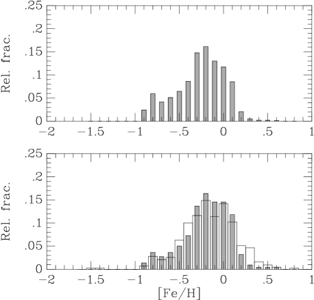
Figure 14: Normalised metallicity distribution functions (MDF) for our K dwarfs. The metallicities are based on [Fe/H]_KF from Table 3. Lower panel : the open histogram is for the basic sample of 431 K dwarfs, selected in the absolute magnitude window $5.5<M_{V}<7.3$. The filled histogram shows the raw normalised MDF for 220 K dwarfs selected to lie in the mass range $0.75<$ M/M${}_{\odot}<0.83$ (c.f. Fig. 13). The main effect of restricting the stars by mass is to remove some stars in the metal rich tail of the distribution. Upper panel : our final normalised metallicity distribution of K dwarfs in the vertical column at the Sun (i.e. including the velocity correction). This histogram is tabulated in Table 5.

Table 5: Tabulated metallicity distribution function for the final sample of 220 K dwarfs, corrected from local density to coloumn density (via the metallicity-velocity dispersion relation) and selected in the mass range $0.75<$ M/M${}_{\odot}<0.83$. This is the MDF shown in the upper panel of Fig 14. The metallicities come from [Fe/H]_KF in Table 3. The error in the relative fractions is based on the Poisson sampling noise in the raw metallicity distribution.

[Fe/H]	Rel. Frac	Error	[Fe/H]	Rel. Frac	Error
$-1.05$	0.0000	-	$-0.15$	0.1304	0.0230
$-0.95$	0.0238	0.0133	$-0.05$	0.1178	0.0208
$-0.85$	0.0590	0.0206	$0.05$	0.0860	0.0168
$-0.75$	0.0411	0.0165	$0.15$	0.0207	0.0077
$-0.65$	0.0507	0.0177	$0.25$	0.0052	0.0035
$-0.55$	0.0643	0.0192	$0.35$	0.0023	0.0021
$-0.45$	0.0859	0.0213	$0.45$	0.0020	0.0018
$-0.35$	0.1475	0.0268	$0.55$	0.0017	0.0016
$-0.25$	0.1615	0.0268	$0.65$	0.0000	-

6 Galactic chemical evolution and K dwarfs

6.1 The theoretical model

The model of Galactic chemical evolution we adopt here is that of Chiappini et al (1997) subsequently modified in Chiappini et al (2001), where a detailed description can be found. We review here the main ingredients of this model:

• The model assumes that the halo + thick disc and the thin disc are formed during two different infall episodes. The thin disc does not form out of gas shed from the halo and the thick disc, but simply out of external gas. Such an interpretation is supported by recent dynamical and kinematical studies of stars in the outer Galactic halo by Sommer-Larsen et al (1997). Under these hypotheses, the infall rate is

  $${dG_{i}(r,t)\over dt} = {A(r)\times{(X_{inf})_{i}e^{-t/\tau_{T}}\over\sigma_{Tot}(r,t_{G})}}~{}~{}+$$ (6)

  $${B(r)\times{(X_{inf})_{i}e^{-(t-t_{max})/\tau_{D}(r)}\over\sigma_{Tot}(r,t_{G})}}$$

  where $\tau_{T}$ represents the time scale for the formation of the halo and the thick disc, and $\tau_{D}(r)$ represents the time scale for disc formation, which is assumed to increase with Galactocentric distance. The best-fit model of Chiappini et al (2001) suggests that the timescale for the formation of the halo and thick disc is quite short and lie in the range $\sim 0.5-1.0$ Gyr, whereas the timescale for the formation of the thin disc is quite long ($\sim 7.0$ Gyr for the solar vicinity). This timescale for the thin disc ensures a very good fit of the new data on the G-dwarf metallicity distribution (Wyse and Gilmore, 1995; Rocha-Pinto and Maciel, 1996). $A(r)$ and $B(r)$ are derived by the condition of reproducing the present total surface mass density distribution in the solar vicinity. In other words, we integrate Eqn. 6 over time up to the present and normalise the left hand side by imposing that it is consistent with the disc’s present total surface mass density. $(X_{inf})_{i}$ is the abundance of the element $i$ in the infalling material, $T_{G}$ the age of the Galaxy, assumed to be 14 Gyr and $t_{max}$ is the time of maximum gas accretion onto the disc coincident with the end of the halo-thick disc phase.

• The Galactic thin disc is approximated by several independent rings, 2 kpc wide, without exchange of matter between them. Continuous infall of gas ensures the temporal increase of the surface mass density $\sigma_{Tot}$ in each ring.

• The instantaneous recycling approximation is relaxed. This is of fundamental importance in treating those isotopes, such as ¹⁴N and ⁵⁶Fe, which are mostly produced by long-lived stars.

• The prescription for the star formation rate (SFR) is:

  $$SFR\propto\sigma_{Tot}^{k_{2}}\sigma_{g}^{k_{1}}$$ (7)

  where $\sigma_{Tot}$ is the total surface mass density and $\sigma_{g}$ is the surface gas density and $k_{1}=1.5$ and $k_{2}=0.5$. A threshold in the surface gas density is also assumed; when the gas density drops below this threshold the star formation stops. Two different values for the gas density threshold are assumed for the halo-thick disc ($\sim 4~{}M_{\odot}pc^{-2}$) and the thin-disc ($\sim 7~{}M_{\odot}pc^{-2}$) phases. The existence of such a threshold has been suggested by star formation studies (Kennicutt, 1989).

• For the initial mass function (IMF) we adopt the prescriptions of Scalo (1986).

• The contributions to the chemical enrichment from supernovae of different type (Ia, Ib and II) as well as from stars dying as C-O white dwarfs and contributing processed and unprocessed elements through stellar winds and the planetary nebula phase are taken into account in great detail (see Chiappini et al, 2001).

• The adopted nucleosynthesis prescriptions are from: (a) van den Hoek and Groenewegen (1997) for low and intermediate stellar masses and (b) Thielemann et al (1993) and Nomoto et al (1997) for SNe Ia. For the massive stars we considered the yields of Woosley and Weaver (1995) (case B) which include explosive nucleosynthesis.

6.2 Observational and Cosmic scatter

The model computes the metallicity distribution function (MDF) assuming no observational or cosmic scatter. The observational scatter in the metallicities for the K dwarfs is 0.1 dex (see section 4.5). This is quite small relative to the width of the observed MDF; the model can be easily convolved to take this into account when comparing to the data.

Potentially more important is the cosmic, or intrinsic scatter, in the metallicities of co-eval stars. There is unfortunately no clear consensus presently regarding the amount of cosmic scatter.

Edvardsson et al. (1993) found that the age-metallicity relation for F and G dwarf stars in the solar neighborhood shows a scatter of order 0.2 dex, which was larger than expected considering the uncertainties in metallicities and ages. This is of the order the width of the MDF, i.e. most of the MDF is accounted for by cosmic scatter, and the increase in the mean metallicity as a function of time plays a minor role.

However, as discussed by Garnett and Kobulnicky (2000) the large scatter found for the stars in the solar vicinity is inconsistent with the abundance measurements in nearby spiral and irregular galaxies (e.g. Kobulnicky and Skillman, 1996) and in the local ISM (Meyer, Jura and Cardelli, 1998), which show that dispersions in ISM abundances are rather small on kiloparsec scales or less. By reanalyzing the Edvardsson et al. sample together with Hipparcos parallaxes and new age estimates, Garnett and Kobulnicky (2000) found that the scatter in the age-metallicity relation depends on the distance to the stars in the sample. They concluded that the intrinsic dispersion in metallicity at fixed age is less than 0.15 dex for field stars in the solar neighbourhood, which is closer to the estimate of less than 0.1 dex for Galactic open star clusters and the ISM (Twarog et al. 1997).

Feltzing, Holmberg and Hurley (2001) argue also this view from a sample 5828 Hipparcos stars for which they derive metallicities and ages; they find a large scatter in metallicity at any given age and even question the existance of the Age-Metallicity Relation itself. Rocha-Pinto et al (2000) argue for a very small cosmic scatter, $\approx 0.1$ dex, based on the age-metallicity relation they present for nearby stars.

As is well known (Pagel and Tautvaisiene, 1995) the metallicity distribution function is a very poor test of the Age-Metallicity relation, so we cannot resolve this issue here. We note that the AMR is less robust than the MDF. In the case of the MDF both quantities are directly observable (number of stars and metallicity), while in the case of the AMR the age scatter contributes significantly to the apparent metallicity scatter and is not easy to quantify. We will take the view that the amount of cosmic scatter is uncertain and we will keep it as a free parameter in the model fitting.

6.3 Model comparison with the K dwarfs

The metallicity distribution function for the model is compared to the data in Fig 15. The model is a good fit. The data are shown in all panels by circles and with error bars based on the Poissonian sampling error (for the 220 star sample). The solid line shows the model results based on the Woosley and Weaver (1995) and van den Hoek and Groenewegen (1997) yields. This model is normalized to the value of the metallicity after $14.0-4.5$ Gyr (i.e. when the Sun was born). In the lower left panel of Fig 15 the curves show the unconvolved model. In the remaining panels the model is convolved by a Gaussian representing the observational and cosmic scatter. The effect of the observational scatter alone is shown in the lower right panel (0.1 dex). The upper left panel shows the convolved model for a total scatter of 0.15 dex, equivalent to 0.1 dex observational scatter and 0.11 dex of cosmic scatter, and the upper right panel shows a total scatter of 0.2 dex, equivalent to 0.1 dex observational scatter and 0.17 dex of cosmic scatter. Clearly, for this model, we cannot constrain the cosmic scatter beyond noting that it is less than 0.2 dex, and probably less than 0.15 dex. This is consistent with existing direct observational constraints (section 6.2. We conclude that the agreement of the model prediction with the observed K-dwarf distribution is excellent, for any reasonable adopted cosmic scatter. An independent analysis of the width of the main sequence in the Hipparcos colour magnitude diagram by Girardi (2002, private communication) has also obtained the result that the cosmic abundance scatter is probably less than 0.2 dex.

Figure 15: Comparison of the model predictions and the metallicity distribution for K dwarfs. In all panels the data are shown by circles. The lower left panel shows the two models, unconvolved, as discussed in the text. The remaining panels show the model convolved with a Gaussian representing the amount of observatinal scatter and intrinsic scatter.

7 Summary

We have calibrated several photometric abundance indices for K dwarfs based on a sample of 34 G and K dwarfs with accurate, spectroscopically determined metallicities. Two of the indices use Cousins $R-I$ photometry to estimate stellar effective temperature and the Geneva $b_{1}$ or Strömgren $m_{1}$ and $c_{1}$ colours. These indices give metallicity estimates of $\approx 0.2$ dex accuracy. A third metallicity index uses $B-V$ and $V-I$ broadband colours. A fourth metallicity index, described in detail in a companion paper (Kotoneva, Flynn and Jimenez 2002, paper II), is based on absolute magnitude $M_{V}$ and $B-V$ colour. These latter two indices appear to provide metallicities of $\approx 0.1$ dex accuracy.

For a set of newly acquired observations of K dwarfs, we use one of these indices to obtain the metallicity distribution of a near complete sample of K dwarfs in the Solar neighbourhood drawn from the Hipparcos catalog. Care has been taken to remove the multiple stars from the sample, for which metallicities cannot be measured accurately. Through isochrones we assign masses to the K dwarfs, and select those K dwarfs which fall into a mass window $0.75<$ M/M${}_{\odot}<0.83$, within which the sample is near to complete. This yields a sample of 220 K dwarfs.

The metallicity distribution of the 220 K dwarfs is strongly peaked near the solar metallicity, confirming the existence of the “G dwarf problem” amongst K dwarfs, as seen in several earlier studies (Marsakov and Shevelev (1988), Flynn and Morell (1997) and Rocha-Pinto and Maciel (1998). We compare the metallicity distribution with Galactic chemical evolution models of Chiappini et al (2001). In the context of this model of the metallicity evolution, we find that the amount of cosmic scatter in the metallicities is small, not more than 0.15 dex. The model match the data well, indicating that the disc was formed via infall processes over an extended time scale of order 7 Gyr.

References

- [] Bessell, M., 1990, A&AS, 83, 357
- [] Campbell B., 1984, ApJ, 283, 209.
- [] Chang, R.X., Hou, J.L., Shu, C.G., Fu, C.Q. 1999, A&A, 350, 38
- [] Chiappini, C., Matteucci, F., Gratton, R., 1997, ApJ, 477, 765
- [] Chiappini, C., Matteucci, F., Romano, D., 2001, ApJ, 554, 1044
- [] Crawford, D.L., Barnes, J.V., 1970, AJ, 75, 978
- [] Edvardsson B., Andersen, J., Gustafsson. B., Lambert, D.L., Nissen, P., Tomkin, J., 1993, A&A, 275, 101
- [] ESA, 1997, The Hipparcos and Tycho Catalogues, ESA, SP-1200
- [] Feltzing S., Holmberg J., Hurley J. R., 2001, A&A, 377, 911.
- [] Flynn, C., Morell, O., 1997, MNRAS, 286, 617
- [] Garnett, D. R., Kobulnicky, H. A., 2000, ApJ, 532, 1192
- [] Gliese, W., Jahreiß, H., 1991, Third Catalogue of Nearby Stars. Astron. Rechen-Inst., Heidelberg (CNS3)
- [] Gould, A., Flynn, C., Bahcall, J., 1998, ApJ, 503, 798
- [] Graham, J.A., 1982, PASP, 94, 244
- [] Grønbech, B., Olsen, E.H., Strömgren, B., 1976, AAS, 26, 155
- [] Hauck, B., Mermilliod, M., 1998, A&AS, 129, 431
- [] Haywood, M., 2001, MNRAS, 325, 1365
- [] Holmberg, J. 2000, PhD thesis, Lund Observatory
- [] Holmberg, J., Flynn, C., 2000, MNRAS, 313, 209
- [] Jimenez, R., Flynn C., Kotoneva, E., 1998, MNRAS, 299, 515
- [] Kennicutt, R.C., 1989, ApJ, 344, 685
- [] Kobulnicky, Henry A., Skillman, Evan D., 1996, ApJ, 471, 211
- [] Kotoneva, E., Flynn, C., Jimenez, R., 2002, accepted to MNRAS (Paper II)
- [] Landolt, A., 1983a, AJ, 88, 439
- [] Landolt, A., 1983b, AJ, 88, 853
- [] Landolt, A., 1992, AJ, 104, 340
- [] Leggett, S., Allard, F., Dahn, C., Hauschildt, P.H., Kerr, T. Rayner, J. 2000, ApJ, 535, 965
- [] Marsakov V.A., Shevelev Yu.G., 1988, BICDS, 35, 129
- [] Menzies, J.W., Cousins, A.W.J., Banfield R.M., Laing J.D., 1989, SAAOC, 13, 1
- [] Meyer, D.M., Jura, M., Cardelli, J.A., 1998, ApJ, 493, 222
- [] Mould, J., 1976, MNRAS, 177, 47
- [] Nomoto, K., Iwamoto, K., Nakasato, N.T., Thielemann F.K., Brachwitz, F., Tsujimoto, T., Kubo, Y., Kishimoto, N., 1997, Nucl. Phys. A, 621, 467c
- [] Pagel, B.E.J., Patchett, B.E., 1975, MNRAS, 172, 13
- [] Pagel, B.E.J., 1997, “Nucleosynthesis and Chemical Evolution of Galaxies”, Cambridge University Press
- [] Pagel B. E. J., Tautvaisiene G., 1995, MNRAS, 276, 505.
- [] Portinari, L., Chiosi, C., Bressan, A., 1998, A&A, 334, 505
- [] Prantzos, N., Silk, J., 1998, ApJ, 507, 229
- [] Reid, I.N., 1993, MNRAS, 265, 785
- [] Reid, I.N., 2002, PASP, 114, 306
- [] Rocha-Pinto, H.J, Maciel, W.J., 1996, MNRAS, 279, 447
- [] Rocha-Pinto, H.J, Maciel, W.J., 1998a, MNRAS, 298, 332
- [] Rocha-Pinto, H.J, Maciel, W.J., 1998b, A&A, 339, 791 (RPM98)
- [] Rocha-Pinto H. J., Maciel W. J., Scalo J., Flynn C., 2000, A&A, 358, 850.
- [] Rufener, F.,1989, A&AS, 78, 469
- [] Scalo, J.M., 1986, Fundam. Cosmic Phys., 11, 1
- [] Schmidt, M., 1963, ApJ, 137, 758
- [] Soederhjelm, S., 1999, A&A, 341, 121
- [] Sommer-Larsen J., 1991, MNRAS, 249, 368.
- [] Sommer-Larsen, J., Beers, T.C., Flynn, C., Wilhelm, R., Christensen, P.R., 1997, ApJ, 481, 775
- [] Stauffer, J., Hartmann, L., 1986, ApJSupp, 61, 531
- [] Taylor, B., 1994, PASP, 106, 600
- [] Thielemann, F.K., Nomoto., K., Hashimoto, M., 1993, in Origin and Evolution of the Elements., Eds. Prantzos, N., Vangioni-Flam, E., Cassé, (Cambridge: Cambridge University Press, 297)
- [] Twarog B. A., Ashman K. M., Anthony-Twarog B. J., 1997, AJ, 114, 2556
- [] van den Bergh, S., 1962, AJ, 67, 486
- [] van den Hoek., l.B., Groenewegen, M.A.T., 1997, A&A, 123, 305
- [] Worthey, G., Dorman, B., Jones, L.A., 1996, AJ, 112, 948
- [] Wilson, O., 1976, ApJ, 205, 823
- [] Wilson, O., Bappu, M.V.K., 1957, ApJ, 125, 661
- [] Wyse, R.F.G., Gilmore, G., 1995, AJ, 110, 2771
- [] Woosley, S.E., Weaver, T.A., 1995, ApJS, 101, 181
- [] Yi, S., Demarque, P., Kim, Y.-C., Lee, Y.-W., Ree, C., Lejeune, Th., Barnes,S., 2001, ApJS, 136, 417