Linear Gas Dynamics in the Expanding Universe: Why the Jeans Scale does not Matter

Abstract

We investigate the relationship between the dark matter and baryons in the linear regime. This relation is quantified by the so-called “filtering scale”. We show that a simple gaussian ansatz which uses the filtering scale provides a good approximation to the exact solution.

1 Introduction

If humans had dark matter vision, cosmology would be a solved problem by now. However, this is not the case, and in our attempt to understand the distribution of matter in the universe we need to rely on baryons - stars and gas - that trace the underlying distribution of the dark matter.

The baryons, though, are not the perfect tracer, since they are subject to other forces in addition to gravity. In this paper we restrict our attention to the linear regime, but even in this simplest physical situation the relationship between the dark matter and baryons (i.e. cosmic gas) is nontrivial, because gas pressure will erase fluctuations on small scales.

The effect of gas pressure on small fluctuations is canonically described by the Jeans scale, which is defined as the scale at which the gravity force equals the gas pressure force. On large scales gravity wins, and small fluctuations grow exponentially, while on small scales, gas pressure turns all fluctuations into sound waves.

However, in the expanding universe the Jeans scale becomes essentially irrelevant, because gravitational instability leads only to slow, power-law growth of fluctuations. Let us consider the following simple thought experiment: in a universe with linear dark matter fluctuations, the gas is instantaneously heated to high temperature. The Jeans scale also increases by a large factor instantaneously, whereas it takes about a Hubble time for the fluctuations in the gas to respond to the changed pressure force. Thus, the instantaneous value of the Jeans scale does not correspond to the characteristic scale over which the fluctuations are suppressed, but instead the suppression scale - which we call the “filtering” scale following Gnedin & Hui (1998) - depends on the whole previous thermal history. Only in the unphysical case of temperature evolving as an exact power-law of the scale factor at all times does the Jeans scale become proportional to the filtering scale (Bi, Borner, & Chu 1992; Fang et al. 1993). However, incorrect expressions for the pressure force filtering have been used even until quite recently (c.f. Choudhury, Padmanabhan, & Srianand 2001)

In this paper we investigate the role of the filtering scale further. Specifically, it has been suggested (Gnedin & Hui 1998; Gnedin 1998) that the relationship between the gas density fluctuation $\delta_{B}$ and the dark matter fluctuation $\delta_{X}$ in the Fourier domain can be approximated by the following simple expression:

$${\delta_{B}\over\delta_{X}}=e^{\displaystyle-k^{2}/k_{F}^{2}},$$ (1)

where $k$ is a wavenumber, and $k_{F}$ is the wavenumber corresponding to the filtering scale. Our goal will be to investigate the range of validity of this approximation.

2 Linear Dynamics in the Expanding Universe

The linear evolution of fluctuations in the expanding universe containing dark matter and cosmic gas is described by two second-order differential equations (Peebles 1980),

$${d^{2}\delta_{X}\over dt^{2}}+2H{d\delta_{X}\over dt} = 4\pi G\bar{\rho}(f_{X}\delta_{X}+f_{B}\delta_{B}),$$

$${d^{2}\delta_{B}\over dt^{2}}+2H{d\delta_{B}\over dt} = 4\pi G\bar{\rho}(f_{X}\delta_{X}+f_{B}\delta_{B})$$ (2)

$$\phantom{AAAA}-{c_{S}^{2}\over a^{2}}k^{2}\delta_{B},$$

where $\delta_{X}(t,k)$ and $\delta_{B}(t,k)$ are Fourier components of density fluctuations in the dark matter and cosmic gas, which have respective mass fractions $f_{X}$ and $f_{B}$, $H(t)$ is the Hubble constant, $a(t)$ is the cosmological scale factor, $\bar{\rho}(t)$ is the average mass density of the universe, $c_{S}(t)$ is the sound speed in the cosmic gas (where the sound speed is simply defined by $c_{S}^{2}\equiv dP/d\rho$, assuming an equation of state that relates the $P$ and $\rho$), $k$ is the comoving wavenumber and $t$ is the proper time.

On large scales ($k\rightarrow 0$) the relationship between the fluctuations in the gas and in the dark matter can be expanded as

$${\delta_{B}(t,k)\over\delta_{X}(t,k)}=1-{k^{2}\over k_{F}^{2}}+O(k^{4}),$$ (3)

where $k_{F}$ is the filtering scale and in general is a function of time.

The filtering scale is related to the Jeans scale $k_{J}$,

$$k_{J}\equiv{a\over c_{S}}\sqrt{4\pi G\bar{\rho}},$$ (4)

by the following relation:

$${1\over k_{F}^{2}(t)} = {1\over D_{+}(t)}\int_{0}^{t}dt^{\prime}{\ddot{D}_{+}(t^{\prime})+2H(t^{\prime})\dot{D}_{+}(t^{\prime})\over k_{J}^{2}(t^{\prime})}$$ (5)

$$\phantom{AAAAA}a^{2}(t^{\prime})\int_{t^{\prime}}^{t}{dt^{\prime\prime}\over a^{2}(t^{\prime\prime})},$$

where $D_{+}(t)$ is the linear growing mode in a given cosmology (Gnedin & Hui 1998).

Inspection of equation (5) shows that the filtering scale as a function of time is related to the Jeans scale as a function of time, but at a given moment in time those two scales are unrelated and can be very different. Thus, given the Jeans scale at a specific moment in time, nothing can be said about the scale over which the fluctuations in the gas are suppressed. It is only when the whole time evolution of the Jeans scale up to some moment in time is known that the filtering scale at this moment can be uniquely defined.

Figure 1: Schematic representation of our parametrization of the thermal history.

In order to investigate the properties of equations (2) as a function of the thermal history of the universe, we parameterize the evolution of the sound speed (as a function of cosmological redshift $z$) in the following way. Before the beginning of reionization at $z=z_{\rm BEG}$ the sound speed is much smaller than the sound speed in the photoionized intergalactic medium (IGM), and is set to zero. Between $z_{\rm BEG}$ and $z_{\rm REI}$ the temperature in the IGM rises linearly with redshift. The sound speed reaches a maximum at the moment of reionization $z_{\rm REI}$ with the value of $c_{S,{\rm REI}}$, after which moment it falls off as $(1+z)^{\beta/2}$. This parametrization is schematically illustrated in Figure 1. Thus, our thermal history is parametrized with 4 parameters: $z_{\rm BEG}$, $z_{\rm REI}$, $c_{S,{\rm REI}}$, which we replace with the mean temperature at reionization in units of $10^{4}\mbox{\,K}$, $T_{4,\rm REI}$, and $\beta$. We adopt a flat cosmological model as our background cosmology, which introduces two more parameters: $\Omega_{0}$ and $\Omega_{B}$. We adopt the following values as our fiducial model:

$$\Omega_{0} = 0.3$$

$$\Omega_{B} = 0$$

$$T_{4,\rm REI} = 2.5$$

$$z_{\rm REI} = 7$$

$$z_{\rm BEG} = 10$$

$$\beta = 1.$$ (6)

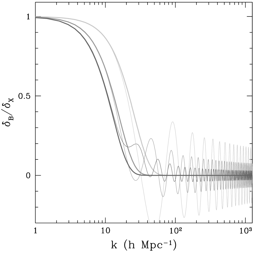
Figure 2: Solutions to equations (2) for our fiducial model at $z=4$ (light grey), $z=1.5$ (medium grey), and $z=0$ (dark grey): thin lines show the exact solutions, thick lines give the approximation (1).

Solutions to equations (2) at three different redshifts are shown in Figure 2 with thin lines. As can be expected, on large scales ($k\rightarrow 0$) the gas follows the dark matter, whereas on small scales oscillations in the gas turn into slowly decaying sound waves. We also show with thick lines the gaussian approximation (1) to illustrate its level of accuracy for our fiducial model. Clearly, the gaussian approximation does not reproduce the small scale oscillations, but it appears to do a decent job in reproducing the transitional region between large and small scales.

3 Results

In this section we present our investigation of the accuracy of the gaussian approximation (1). Our approach to testing the approximation is motivated by its applicability. We can envision using the approximation as a simpler way of computing the rms density fluctuations in the gas:

$$\sigma^{2}_{B}(t)={1\over 2\pi^{2}}\int_{0}^{\infty}P_{X}(k)\left[\delta_{B}(t,k)\over\delta_{X}(t,k)\right]^{2}k^{2}dk\approx$$

$$\approx{1\over 2\pi^{2}}\int_{0}^{\infty}P_{X}(k)e^{\displaystyle-2k^{2}/k_{F}^{2}(t)}k^{2}dk,$$ (7)

where $P_{X}(k)$ is the dark matter power spectrum. Another use of the approximation could be in giving the shape of the gas power spectrum on small scales:

$$P_{B}(k,t)=P_{X}(k)\left[\delta_{B}(t,k)\over\delta_{X}(t,k)\right]^{2}\approx$$

$$\approx P_{X}(k)e^{\displaystyle-2k^{2}/k_{F}^{2}(k)}.$$ (8)

Thus, our goal is to estimate the accuracy of the gaussian approximation both in equation (7) and in equation (8) in our six-dimensional parameter space.

A full sampling of this parameter space would be unrealistic, so we focus on varying two of the parameters at a time, keeping the rest of the parameters fixed to our fiducial values. For the dark matter power spectrum $P_{X}(k)$, we adopt a canonical Cold Dark Matter + Cosmological Constant power spectrum with $\Omega_{0}h=0.25$, Harrison-Zel’dovich scale-free primordial spectrum, and the BBKS transfer function (Bardeen et al. 1986).

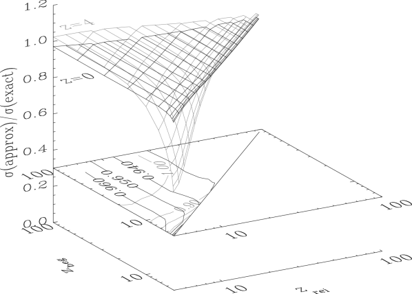
Figure 3: The accuracy of the gaussian approximation in computing the rms gas fluctuation as a function of $z_{\rm REI}$ and $z_{\rm BEG}$ at $z=4$ (grey) and $z=0$ (black).

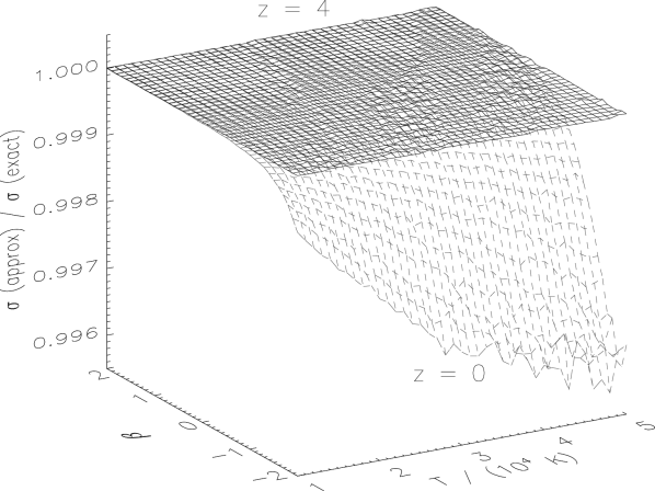
Figure 4: The same as Fig. 3, except as a function of $T_{4,\rm REI}$ and $\beta$.

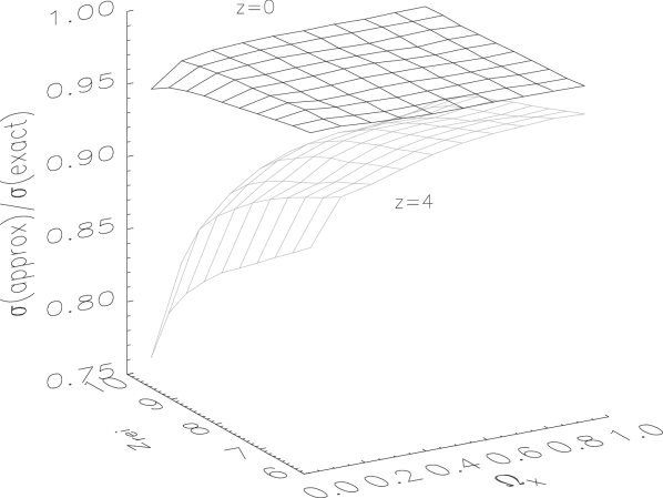
Figure 5: The same as Fig. 3, except as a function of $\Omega_{X}$ and $z_{\rm REI}$ (with $z_{\rm BEG}$ begin kept fixed at 10).

Figure 6: The same as Fig. 3, except as a function of $\Omega_{X}$ and $\Omega_{B}$.

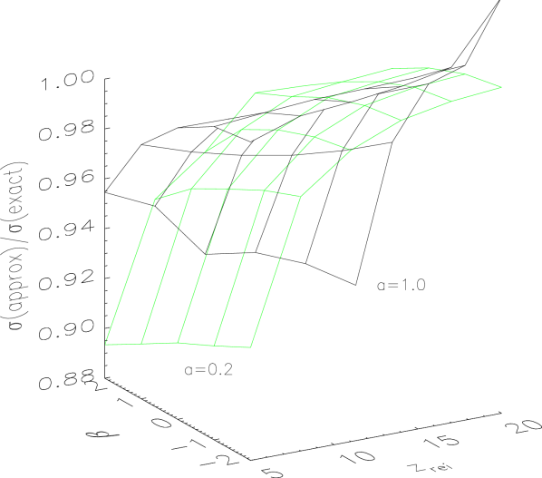
Figure 7: The same as Fig. 3, except as a function of $z_{\rm REI}$ and $\beta$.

The choice of the power spectrum does matter. For example, if the power spectrum contains a lot of power on very small scales (below the filtering scale), then oscillations shown in Fig. 2 will be amplified, which, in turn, will compromise the approximation (1). However, we believe that the dark matter power spectrum is known sufficiently well up to scales of interest, so our choice is justified.

Figures 3-6 show the accuracy of the gaussian approximation as a function of our parameters. One can see that in general the approximation holds very well, with the approximate $\sigma_{B}$ being within 10% of the exact value. The approximation breaks down at $z\gtrsim 4$ in the limit when reionization is quite fast ($z_{\rm BEG}\lesssim 1.2z_{\rm REI}$) and the redshift of reionization is low ($z_{\rm REI}<6$). It also gets somewhat worse for very low values of $\Omega_{0}$. This is not surprising, since in those two regimes the oscillations at large $k$ are substantial and make a non-negligible contribution to the integral (7).

We have also found that in essentially all cases the gaussian approximation gives a better than 20% (10% in amplitude) fit to the gas power spectrum (8) for $k<0.9k_{F}$.

4 Conclusions

We have shown that the gaussian approximation (1) provides a reasonably good fit (better than 10%) to the rms density fluctuations in the gas, and for the shape of the gas power spectrum for $k<0.9k_{F}$. It is important to underscore that there is no known physical reason why this approximation works so well, so it should be considered as a mathematical coincidence. Notwithstanding, the gaussian approximation can be used in semianalytical models of the Lyman-alpha forest and early universe, when a full solution to equations (2) is not practical.

References

- (1)
- (2) Bardeen, J. M., Bond, J. R., Kaiser, N., & Szalay, A. S. 1986, ApJ, 304, 15
- (3)
- (4) Bi, H. G., Borner, G., & Chu, Y. 1992, A&A, 266, 1
- (5)
- (6) Choudhury, T. R., Padmanabhan, T., & Srianand, R. 2001, MNRAS, 322, 561
- (7)
- (8) Choudhury, T. R., Srianand, R., & Padmanabhan, T. 2001, ApJ, 559, 29
- (9)
- (10) Fang, L. Z., Bi, H., Xiang, S., & Boerner G., 1993, ApJ, 413, 477
- (11)
- (12) Gnedin, N. Y., & Hui, L. 1998, MNRAS, 296, 44
- (13)
- (14) Gnedin, N. Y. 1998, MNRAS, 299, 392
- (15)
- (16) Peebles, P. J. E. 1980, The Large-Scale Structure of the Universe (Princeton: Princeton University Press)
- (17)