Reformulation of Smoothed Particle Hydrodynamics
with Riemann Solver

Abstract

Smoothed Particle Hydrodynamics is reformulated in terms of the convolution of the original hydrodynamics equations, and the new evolution equations for the particles are derived. The same evolution equation of motion is also derived using a new action principle. The force acting on each particle is determined by solving the Riemann problem. The use of the Riemann Solver strengthens the method, making it accurate for the study of phenomena with strong shocks. The prescription for the variable smoothing length is shown. These techniques are implemented in strict conservation form. The results of a few test problems are also shown.

Journal of Computational Physics jcph.2002.7053 2002 Shu-ichiro Inutsuka SPH with Riemann Solver

1 Introduction

Smoothed particle hydrodynamics (SPH, [14, 7]) is a fully Lagrangian particle method to describe the hydrodynamical phenomena. The Lagrangian particle methods are especially suited to hydrodynamical problems that have large empty regions and moving boundaries. Those problems naturally arise in engineering science as well as geophysics and astrophysics. A variety of astrophysical problems have been studied by SPH because of its simplicity in programming the two- and three-dimensional codes and its versatility of incorporating the various physical effects such as self-gravity, radiative cooling, and chemical reactions. A broad discussion of the method can be found in a review by Monaghan [18]. However, the inconsistency of the method is emphasized by Dilts [3, 4] who modified the method by means of the moving-least-square basis functions to obtain accurate derivatives regardless of the positions of the SPH particles. Another concern of the method is its poor description of the strong shocks. In the two- or three-dimensional calculation of colliding gases, particles often penetrate into the opposite side. This unphysical effect can be partially eliminated by the so-called XSPH prescription [17] that does not introduce the (required) additional dissipation but results in the additional dispersion of the waves. Therefore it is very desirable to construct a method that is simple and able to describe the strong shock phenomena accurately.

In this paper, a new method for handling shocks in particle hydrodynamics is constructed. The force acting on each particle is determined by solving the Riemann problem (RP). This use of the so-called Riemann Solver is introduced as an simple analogy of the grid-based method [6]. The previous attempts to introduce Riemann Solver into the particle method failed to give the method an exact conservation form [9, 10]. This paper describes how to include the exact Riemann Solver into the strictly conservative particle method.

The alternative approach to including small but sufficient dissipation into the numerical solution is to find a good limiter to switch a dissipative method and a less-dissipative method [5, 21]. In principle, however, the switch is always an option to any numerical scheme including the present one, and its discussion is beyond the scope of this paper.

Section 2 provides a description of the method where we derive the evolution equations for the particles in terms of the convolution of the original hydrodynamic equations with the so-called kernel function. The same evolution equations are derived from an action principle which is different from the previous ones [19, 20], which sheds light on the “hidden” approximation in the expression for the velocity field in SPH formalism. The detailed explanation for the implementation is described in Section 3. The usage of the Riemann Solver is analogous to the grid-based second-order Godunov scheme [24]. A variable smoothing length is also considered. Numerical examples involving strong shocks are presented in Section 4. Section 5 is for summary.

2 The Method

We consider the following set of equations for non-radiating inviscid fluid:

$$\frac{d\rho}{dt}=-\rho\nabla\cdot\mbox{\boldmath$v$},$$ (1)

$$\frac{d\mbox{\boldmath$v$}}{dt}=-\frac{1}{\rho}\nabla P,$$ (2)

$$\frac{du}{dt}=-\frac{P}{\rho}\nabla\cdot\mbox{\boldmath$v$},$$ (3)

$$P=(\gamma-1)\rho u,$$ (4)

where $u$ denotes the specific internal energy, $\gamma$ denotes the ratio of specific heats, and other symbols have their usual meanings.

In the standard SPH method, each particle has its own mass, and density at each particle’s location is simply assigned by

$$\rho_{i}=\sum_{j}m_{j}W(\mbox{\boldmath$x$}_{i}-\mbox{\boldmath$x$}_{j},h),$$ (5)

where subscripts denote particle labels, $m_{j}$ is the mass of the $j$-th particle, and $W(\mbox{\boldmath$x$},h)$ is a spherically symmetric kernel function which is normalized to be unity if integrated in space:

$$W(\mbox{\boldmath$x$},h)=W(-\mbox{\boldmath$x$},h),$$ (6)

$$\int W(\mbox{\boldmath$x$},h)d\mbox{\boldmath$x$}=1,$$ (7)

and $h$ is the parameter of the kernel function. For later convenience we also define the effective width $h_{\rm eff}$ of the kernel function $W(\mbox{\boldmath$x$})$ by

$$h_{\rm eff}^{2}\equiv 2\int x^{2}W(\mbox{\boldmath$x$},h)d\mbox{\boldmath$x$}.$$ (8)

Although there are many possible forms for $W(\mbox{\boldmath$x$},h)$, we use the following Gaussian kernel throughout in this paper:

$$W(\mbox{\boldmath$x$},h)=\left[\frac{1}{h\sqrt{\pi}}\right]^{d}e^{-\mbox{\boldmath$x$}^{2}/h^{2}}.$$ (9)

In the above equation, $d$ is the number of dimensions, and $h$ is the so-called smoothing length. Note that $h_{\rm eff}=h$ for this Gaussian kernel. We assume $h$ is constant in space in Sections 2.1-3.2. The spatially variable smoothing length is considered in Section 3.3 and the subsequent Sections.

The standard procedure to derive sets of evolution equations for SPH has been previously described [18]. In the following sections, we show how new evolution equations are derived from the original hydrodynamics equations. We then show that our new equation of motion can be derived from the action principle for an appropriately defined Lagrangian function.

2.1 Key Concept

In general any method of computational fluid dynamics inevitably brings errors into the solutions. Therefore the essential feature of the method can be characterized by how to introduce the errors into the solutions. For example, in many kinds of grid-based methods, the truncation of the Taylor-series expansion is the origin of the errors in the numerical solutions. In the SPH formalism we consider the convolution of the physical function $f(x)$ with the kernel function,

$$\langle f\rangle(\mbox{\boldmath$x$})\equiv\int f(\mbox{\boldmath$x$}^{\prime})W(\mbox{\boldmath$x$}^{\prime}-\mbox{\boldmath$x$},h)d\mbox{\boldmath$x$}^{\prime}.$$ (10)

We use the symbol $\langle\rangle$ to denote the convolution. Taylor-series expansion of $f$ around $\mbox{\boldmath$x$}=\mbox{\boldmath$x$}_{i}$ in Eq.(10) shows that the difference of $\langle f\rangle(\mbox{\boldmath$x$}_{i})$ and $f(\mbox{\boldmath$x$}_{i})$ is the second-order in $h_{\rm eff}$:

$$\langle f\rangle(\mbox{\boldmath$x$}_{i})=f(\mbox{\boldmath$x$}_{i})+\frac{h_{\rm eff}^{2}}{4}\nabla^{2}f(\mbox{\boldmath$x$})+O(h_{\rm eff}^{4}).$$ (11)

Thus if we use $\langle f\rangle$ as an approximate solution for $f$, the errors of the second-order in $h_{\rm eff}$ are introduced by the convolution with the symmetric function $W$.

We also have

$$\langle\frac{\partial f}{\partial x}\rangle(\mbox{\boldmath$x$}) = \int\frac{\partial f(\mbox{\boldmath$x$}^{\prime})}{\partial x^{\prime}}W(\mbox{\boldmath$x$}^{\prime}-\mbox{\boldmath$x$},h)d\mbox{\boldmath$x$}^{\prime}$$ (12)

$$= -\int f(\mbox{\boldmath$x$}^{\prime})\frac{\partial}{\partial x^{\prime}}W(\mbox{\boldmath$x$}^{\prime}-\mbox{\boldmath$x$},h)d\mbox{\boldmath$x$}^{\prime}$$

$$= \frac{\partial}{\partial x}\int f(\mbox{\boldmath$x$}^{\prime})W(\mbox{\boldmath$x$}^{\prime}-\mbox{\boldmath$x$},h)d\mbox{\boldmath$x$}^{\prime},$$

where we used the integration by part and Eq.(6). That is, the kernel convolution of $\nabla f$ is just $\nabla\langle f\rangle$.

If we define the density distribution by the summation of the kernel functions at particle positions:

$$\rho(\mbox{\boldmath$x$})\equiv\sum_{j}m_{j}W(\mbox{\boldmath$x$}-\mbox{\boldmath$x$}_{j},h),$$ (13)

then we have the following identities:

$$1=\sum_{j}\frac{m_{j}}{\rho(\mbox{\boldmath$x$})}W(\mbox{\boldmath$x$}-\mbox{\boldmath$x$}_{j},h),$$ (14)

$$0=\sum_{j}m_{j}\nabla\left[\frac{W(\mbox{\boldmath$x$}-\mbox{\boldmath$x$}_{j},h)}{\rho(\mbox{\boldmath$x$})}\right].$$ (15)

These equations are the key equations in the present method. Using Eq.(14) the value of the kernel convolution can be cast into the following expression:

$$f_{i}\equiv\langle f\rangle(\mbox{\boldmath$x$}_{i}) = \int f(\mbox{\boldmath$x$}^{\prime})W(\mbox{\boldmath$x$}^{\prime}-\mbox{\boldmath$x$}_{i},h)d\mbox{\boldmath$x$}^{\prime}$$ (16)

$$= \int\sum_{j}m_{j}\frac{f(\mbox{\boldmath$x$}^{\prime})}{\rho(\mbox{\boldmath$x$}^{\prime})}W(\mbox{\boldmath$x$}^{\prime}-\mbox{\boldmath$x$}_{i},h)W(\mbox{\boldmath$x$}^{\prime}-\mbox{\boldmath$x$}_{j},h)d\mbox{\boldmath$x$}^{\prime}$$

$$= \sum_{j}\Delta f_{i,j},$$

where we define

$$\Delta f_{i,j}\equiv\int m_{j}\frac{f(\mbox{\boldmath$x$}^{\prime})}{\rho(\mbox{\boldmath$x$}^{\prime})}W(\mbox{\boldmath$x$}^{\prime}-\mbox{\boldmath$x$}_{i},h)W(\mbox{\boldmath$x$}^{\prime}-\mbox{\boldmath$x$}_{j},h)d\mbox{\boldmath$x$}^{\prime}.$$ (17)

Note that $m_{i}\Delta f_{i,j}$ is symmetric with respect to $i$ and $j$. In this way the value ($f_{i}$) of the physical variable $f$ at the $i$-th particle position is expressed as the summation of the contributions ($\Delta f_{i,j}$) from the surrounding particles. This expression shows the spirit of the present method, although the actual detailed evolution equations are presented in the following sections.

In contrast the standard SPH adopts the following form for $\Delta f_{i,j}$:

$$\Delta f_{i,j}\approx m_{j}\frac{f(\mbox{\boldmath$x$}_{j})}{\rho(\mbox{\boldmath$x$}_{j})}W(\mbox{\boldmath$x$}_{i}-\mbox{\boldmath$x$}_{j},h).$$ (18)

This corresponds to the crude approximation, $W(\mbox{\boldmath$x$}_{j}-\mbox{\boldmath$x$}^{\prime},h)\approx\delta(\mbox{\boldmath$x$}^{\prime}-\mbox{\boldmath$x$}_{j})$ in Eq.(17), where $\delta(\mbox{\boldmath$x$})$ is the Dirac’s $\delta$ funcion. The standard SPH also implicitly assumes the following approximate equation:

$$1\approx\sum_{j}\frac{m_{j}}{\rho(\mbox{\boldmath$x$}_{j})}W(\mbox{\boldmath$x$}-\mbox{\boldmath$x$}_{j},h),$$ (19)

instead of Eq.(14), although this is very poor approximation.

In the MLSPH scheme by Dilts, an equation analogous to Eq.(14) is provided by the moving-least-square basis functions, although he needed somewhat heavy operations to construct his basis functions. Note that our method does not restrict the functional form of the kernel function to satisfy Eqs.(13),(14).

2.2 Equation of Motion

To derive the appropriate evolution equation for particles we take the convolution of the equation of motion (EoM), Eq.(2),

$$\int\frac{d\mbox{\boldmath$v$}(\mbox{\boldmath$x$})}{dt}W(\mbox{\boldmath$x$}-\mbox{\boldmath$x$}^{\prime},h)d\mbox{\boldmath$x$}=-\int\frac{1}{\rho(\mbox{\boldmath$x$})}\nabla P(\mbox{\boldmath$x$})~{}W(\mbox{\boldmath$x$}-\mbox{\boldmath$x$}^{\prime},h)d\mbox{\boldmath$x$}.$$ (20)

The right-hand side of this equation can be transformed into the following expression:

$$-\int\left\{\left[\nabla\frac{P(\mbox{\boldmath$x$})}{\rho(\mbox{\boldmath$x$})}\right]W(\mbox{\boldmath$x$}-\mbox{\boldmath$x$}^{\prime},h)+\frac{P(\mbox{\boldmath$x$})}{\rho^{2}(\mbox{\boldmath$x$})}\left[\nabla\rho(\mbox{\boldmath$x$})\right]W(\mbox{\boldmath$x$}-\mbox{\boldmath$x$}^{\prime},h)\right\}d\mbox{\boldmath$x$}$$

$$=\int\left\{\frac{P(\mbox{\boldmath$x$})}{\rho(\mbox{\boldmath$x$})}\nabla~{}W(\mbox{\boldmath$x$}-\mbox{\boldmath$x$}^{\prime},h)-\frac{P(\mbox{\boldmath$x$})}{\rho^{2}(\mbox{\boldmath$x$})}\left[\nabla~{}\sum_{j}m_{j}W(\mbox{\boldmath$x$}-\mbox{\boldmath$x$}_{j},h)\right]W(\mbox{\boldmath$x$}-\mbox{\boldmath$x$}^{\prime},h)\right\}d\mbox{\boldmath$x$}$$

$$=\sum_{j}m_{j}\int\frac{P}{\rho^{2}}\left\{\nabla W(\mbox{\boldmath$x$}-\mbox{\boldmath$x$}^{\prime},h)W(\mbox{\boldmath$x$}-\mbox{\boldmath$x$}_{j},h)-W(\mbox{\boldmath$x$}-\mbox{\boldmath$x$}^{\prime},h)\nabla W(\mbox{\boldmath$x$}-\mbox{\boldmath$x$}_{j},h)\right\}d\mbox{\boldmath$x$}$$

(21)

where we integrated by part and used the identity Eq.(14).

Thus if we adopt the following equation for the evolution of the particle positions,

$$\ddot{\mbox{\boldmath$x$}}_{i}\equiv\int\frac{d\mbox{\boldmath$v$}(\mbox{\boldmath$x$})}{dt}W(\mbox{\boldmath$x$}-\mbox{\boldmath$x$}_{i},h)d\mbox{\boldmath$x$}=-\int\frac{1}{\rho(\mbox{\boldmath$x$})}\nabla P(\mbox{\boldmath$x$})~{}W(\mbox{\boldmath$x$}-\mbox{\boldmath$x$}_{i},h)d\mbox{\boldmath$x$},$$ (22)

we obtain the evolution equation that is consistent and spatially second-order accurate to the original hydrodynamical equation of motion:

$$m_{i}\ddot{\mbox{\boldmath$x$}}_{i}=-m_{i}\sum_{j}m_{j}\int\frac{P(\mbox{\boldmath$x$})}{\rho^{2}(\mbox{\boldmath$x$})}\left[\frac{\partial}{\partial\mbox{\boldmath$x$}_{i}}-\frac{\partial}{\partial\mbox{\boldmath$x$}_{j}}\right]W(\mbox{\boldmath$x$}-\mbox{\boldmath$x$}_{i},h)W(\mbox{\boldmath$x$}-\mbox{\boldmath$x$}_{j},h)d\mbox{\boldmath$x$},$$ (23)

where the overdot means a time-derivative. The antisymmetric appearance of $i$ and $j$ on the right-hand side guarantees the conservation of the linear and angular momentum of the particle system. From this equation we can deduce some properties of the EoM of the particle system. For example, if the pressure distribution is constant in space, the acceleration vanishes exactly in Eq. (23), which is evident in Eq. (22). The evolution equation of MLSPH also has a similar property although the standard SPH does not [3].

In this way the main approximation introduced in the present method is simply expressed in Eq. (22), while the standard SPH formalism does not have such simple explanation.

2.3 Energy Equation

We can follow the evolution of barotropic fluid with $P=P(\rho)$ only by the EoM derived in the previous section. However an additional evolution equation for energy is required to describe the evolution of non-barotropic fluid. The energy equation is also needed to handle shocks. The energy equation guarantees the conservation of the total energy of the system in the absence of other sources or losses of energy, such as radiative heating or cooling. On the other hand, the strict conservation property in the numerical calculation guarantees the accurate description of strong shocks. This is because the structure of shock wave is determined by the Rankine-Hugoniot relation which is the direct consequence of the physical conservation laws. Thus we must derive the energy equation that has strict conservation property and a convenient form to include additional physical dissipation.

As in Eq. (20), we multiply both sides of Eq. (3) by $W(\mbox{\boldmath$x$}-\mbox{\boldmath$x$}^{\prime},h)$, and integrate in space (with respect to $x$),

$$\int\frac{du(\mbox{\boldmath$x$})}{dt}W(\mbox{\boldmath$x$}-\mbox{\boldmath$x$}^{\prime},h)d\mbox{\boldmath$x$}=-\int\frac{P(\mbox{\boldmath$x$})}{\rho(\mbox{\boldmath$x$})}[\nabla\cdot\mbox{\boldmath$v$}]~{}W(\mbox{\boldmath$x$}-\mbox{\boldmath$x$}^{\prime},h)d\mbox{\boldmath$x$}.$$ (24)

The right-hand side of this equation can be transformed into the following expression:

$$-\int\frac{P(\mbox{\boldmath$x$})}{\rho(\mbox{\boldmath$x$})}[\nabla\cdot\mbox{\boldmath$v$}]~{}W(\mbox{\boldmath$x$}-\mbox{\boldmath$x$}^{\prime},h)d\mbox{\boldmath$x$}$$

$$= -\int\frac{1}{\rho(\mbox{\boldmath$x$})}[\nabla\cdot P\mbox{\boldmath$v$}]~{}W(\mbox{\boldmath$x$}-\mbox{\boldmath$x$}^{\prime},h)d\mbox{\boldmath$x$}+\int\frac{1}{\rho(\mbox{\boldmath$x$})}[\mbox{\boldmath$v$}\cdot\nabla P]~{}W(\mbox{\boldmath$x$}-\mbox{\boldmath$x$}^{\prime},h)d\mbox{\boldmath$x$}$$

At this point, we again make an approximation according to the following equation (see also Eqs.(36),(2.4)):

$$\int\frac{1}{\rho(\mbox{\boldmath$x$})}[\mbox{\boldmath$v$}\cdot\nabla P]~{}W(\mbox{\boldmath$x$}-\mbox{\boldmath$x$}_{i},h)d\mbox{\boldmath$x$} = \int\frac{1}{\rho(\mbox{\boldmath$x$})}[\dot{\mbox{\boldmath$x$}}_{i}\cdot\nabla P]~{}W(\mbox{\boldmath$x$}-\mbox{\boldmath$x$}_{i},h)d\mbox{\boldmath$x$}+O(h^{2}).$$

Then we have

$$\dot{u_{i}} \equiv \int\frac{du(\mbox{\boldmath$x$})}{dt}W(\mbox{\boldmath$x$}-\mbox{\boldmath$x$}_{i},h)d\mbox{\boldmath$x$}$$

$$\approx -\int\frac{1}{\rho(\mbox{\boldmath$x$})}[\nabla\cdot P\mbox{\boldmath$v$}]~{}W(\mbox{\boldmath$x$}-\mbox{\boldmath$x$}_{i},h)d\mbox{\boldmath$x$}+\int\frac{1}{\rho(\mbox{\boldmath$x$})}[\dot{\mbox{\boldmath$x$}}_{i}\cdot\nabla P]~{}W(\mbox{\boldmath$x$}-\mbox{\boldmath$x$}_{i},h)d\mbox{\boldmath$x$}$$

$$= \int P[\mbox{\boldmath$v$}-\dot{\mbox{\boldmath$x$}}_{i}]\cdot\nabla\left[\frac{W(\mbox{\boldmath$x$}-\mbox{\boldmath$x$}_{i},h)}{\rho}\right]d\mbox{\boldmath$x$}$$

$$= \sum_{j}m_{j}\int\frac{P}{\rho^{2}}[\mbox{\boldmath$v$}-\dot{\mbox{\boldmath$x$}}_{i}]\cdot\left[\nabla W(\mbox{\boldmath$x$}-\mbox{\boldmath$x$}_{i},h)W(\mbox{\boldmath$x$}-\mbox{\boldmath$x$}_{j},h)\right.$$

$$~{}~{}~{}~{}~{}~{}~{}~{}~{}~{}~{}~{}~{}~{}~{}~{}~{}~{}~{}~{}~{}~{}~{}~{}~{}~{}~{}~{}~{}\left.-W(\mbox{\boldmath$x$}-\mbox{\boldmath$x$}_{i},h)\nabla W(\mbox{\boldmath$x$}-\mbox{\boldmath$x$}_{j},h)\right]d\mbox{\boldmath$x$},$$

where we have again used the identities (14), (15). This form of the energy equation will be further modified to account for the physical dissipation in Section 3.2, and its conservation property will be shown in Section 3.4.

2.4 Action Principle

In this section we show another feature of the equation of motion in the present method. In the case without dissipation, the equation of motion for the particles in our method can be derived from an action principle. Therefore the time evolution of the particle system can be formulated in a canonical transformation, that might further enable the possible improvement of the time integration.

For the moment, we consider barotropic fluid in which pressure is a function of density alone, $P(\rho)=K\rho^{\gamma}$. In this case, the equation of motion (Eq.[2]) for the fluid can be derived by minimizing the action $S$ which is the time integral of the Lagrangian function $L$ expressed in Lagrangian coordinates:

$$S=\int Ldt,$$ (28)

$$L=\int{\cal L}d\mbox{\boldmath$x$}=\int\left[\frac{1}{2}\rho\mbox{\boldmath$v$}^{2}-\rho u\right]d\mbox{\boldmath$x$}.$$ (29)

If we use Eulerian coordinates, the appropriate Lagrangian density $\cal L$ must include constraint equations along with Lagrange multipliers [13, 22], which introduce additional complication. In contrast, the Lagrangian density shown above is simple and analogous to the classical particle mechanics form, owing to the use of Lagrangian coordinates. In addition we can derive the Hamiltonian and the evolution becomes the canonical transformation which is free from dissipation. Although this formalism is for the continuous media, we can use this formalism to derive the evolution equation for the system of particles.

First we consider the density field expressed in the following equation:

$$\rho(\mbox{\boldmath$x$})=\sum_{j}m_{j}W(\mbox{\boldmath$x$}-\mbox{\boldmath$x$}_{j},h).$$ (30)

This continuous distribution of density is defined only by (the finite number of) the positions of particles, $\mbox{\boldmath$x$}_{i}~{}(i=1,2,3,...,N_{\rm p})$. Time-derivative of the above equation gives

$$\frac{\partial\rho(\mbox{\boldmath$x$})}{\partial t}=\sum_{j}m_{j}\dot{\mbox{\boldmath$x$}}_{j}\cdot\frac{\partial}{\partial\mbox{\boldmath$x$}_{j}}W(\mbox{\boldmath$x$}-\mbox{\boldmath$x$}_{j},h)=-\sum_{j}m_{j}\dot{\mbox{\boldmath$x$}}_{j}\nabla W(\mbox{\boldmath$x$}-\mbox{\boldmath$x$}_{j},h)=-\nabla\cdot\mbox{\boldmath$F$}_{\rm m},$$ (31)

where we defined

$$\mbox{\boldmath$F$}_{\rm m}(\mbox{\boldmath$x$})\equiv\sum_{j}m_{j}\dot{\mbox{\boldmath$x$}}_{j}W(\mbox{\boldmath$x$}-\mbox{\boldmath$x$}_{j},h).$$ (32)

Comparing Eq. (31) with the ordinary continuity equation, we realize that $\mbox{\boldmath$F$}_{\rm m}$ defines the mass flux,

$$\mbox{\boldmath$F$}_{\rm m}(\mbox{\boldmath$x$})=\rho(\mbox{\boldmath$x$})\mbox{\boldmath$v$}(\mbox{\boldmath$x$})$$ (33)

From this equation we can deduce the definition of velocity field given by the following equation:

$$\mbox{\boldmath$v$}(\mbox{\boldmath$x$})=\frac{\mbox{\boldmath$F$}_{\rm m}(\mbox{\boldmath$x$})}{\rho(\mbox{\boldmath$x$})}=\frac{\sum_{j}m_{j}\dot{\mbox{\boldmath$x$}}_{j}W(\mbox{\boldmath$x$}-\mbox{\boldmath$x$}_{j},h)}{\sum_{j}m_{j}W(\mbox{\boldmath$x$}-\mbox{\boldmath$x$}_{j},h)}.$$ (34)

Note that at $\mbox{\boldmath$x$}=\mbox{\boldmath$x$}_{i}$ the above equation gives

$$\mbox{\boldmath$v$}(\mbox{\boldmath$x$}_{i})=\dot{\mbox{\boldmath$x$}}_{i}+\frac{1}{\rho_{i}}\sum_{j}m_{j}[\dot{\mbox{\boldmath$x$}}_{j}-\dot{\mbox{\boldmath$x$}}_{i}]W(\mbox{\boldmath$x$}_{i}-\mbox{\boldmath$x$}_{j},h).$$ (35)

The difference of $\mbox{\boldmath$v$}(\mbox{\boldmath$x$}_{i})$ and $\dot{\mbox{\boldmath$x$}}_{i}$ is second order in $h$. In a one-dimensional case, for example, this can be shown by using an appropriate smooth function $f_{x}$ that satisfies $f_{x}(x_{i})=\dot{x}_{i}~{}~{}(i=1,2,...,N_{\rm p})$ as

$$v_{x}(x_{i})-\dot{x}_{i}$$ (36)

$$= \frac{1}{\rho_{i}}\sum_{j}m_{j}\left\{\frac{\partial f_{x}}{\partial x}[x_{j}-x_{i}]+\frac{1}{2}\frac{\partial^{2}f_{x}}{\partial x^{2}}[x_{j}-x_{i}]^{2}+O([x_{j}-x_{i}]^{3})\right\}W(x_{i}-x_{j},h)$$

$$= \frac{1}{\rho_{i}}\frac{h^{2}}{2}\left\{\frac{\partial f_{x}}{\partial x}\frac{\partial\rho}{\partial x}+\frac{1}{2}\frac{\partial^{2}f_{x}}{\partial x^{2}}\rho\right\}+O(h^{4}).$$

Eqs. (30) and (34) can be used for $\mbox{\boldmath$v$}(\mbox{\boldmath$x$})$ and $\rho(\mbox{\boldmath$x$})$ in Eq. (29) to obtain the Lagrangian function that is defined only by the positions of particles.

$$L=\int\left\{\frac{\left[\sum_{j}m_{j}\dot{\mbox{\boldmath$x$}}_{j}W(\mbox{\boldmath$x$}-\mbox{\boldmath$x$}_{j},h)\right]^{2}}{2\sum_{j}m_{j}W(\mbox{\boldmath$x$}-\mbox{\boldmath$x$}_{j},h)}-\frac{K}{\gamma-1}\left[\sum_{j}m_{j}W(\mbox{\boldmath$x$}-\mbox{\boldmath$x$}_{j},h)\right]^{\gamma}\right\}d\mbox{\boldmath$x$}.$$ (37)

This is the exact Lagrangian for the “fluid” of which density and velocity are constrained by Eqs. (30) and (34).

Instead of adopting this complicated Lagrangian function, we now make an approximation for the velocity field by Taylor-series expansion of the velocity field:

$$\mbox{\boldmath$v$}(\mbox{\boldmath$x$}) = \mbox{\boldmath$v$}(\mbox{\boldmath$x$}_{i})+[\mbox{\boldmath$x$}-\mbox{\boldmath$x$}_{i}]\cdot\nabla\mbox{\boldmath$v$}(\mbox{\boldmath$x$}_{i})+O(|\mbox{\boldmath$x$}-\mbox{\boldmath$x$}_{i}|^{2})$$

$$= \dot{\mbox{\boldmath$x$}}_{i}+\frac{1}{\rho_{i}}\sum_{j}m_{j}[\dot{\mbox{\boldmath$x$}}_{j}-\dot{\mbox{\boldmath$x$}}_{i}]W(\mbox{\boldmath$x$}_{i}-\mbox{\boldmath$x$}_{j},h)+[\mbox{\boldmath$x$}-\mbox{\boldmath$x$}_{i}]\cdot\nabla\mbox{\boldmath$v$}(\mbox{\boldmath$x$}_{i})+O(|\mbox{\boldmath$x$}-\mbox{\boldmath$x$}_{i}|^{2}).$$

From this we have

$$\int\mbox{\boldmath$v$}(\mbox{\boldmath$x$})W(\mbox{\boldmath$x$}-\mbox{\boldmath$x$}_{i},h)d\mbox{\boldmath$x$}=\dot{\mbox{\boldmath$x$}}_{i}+O(h^{2}).$$ (39)

With this equation we can simplify the kinetic term of Lagrangian function as follows:

$$\int\frac{1}{2}\rho\mbox{\boldmath$v$}^{2}d\mbox{\boldmath$x$} = \frac{1}{2}\int\mbox{\boldmath$F$}_{\rm m}\cdot\mbox{\boldmath$v$}d\mbox{\boldmath$x$}$$ (40)

$$= \frac{1}{2}\sum_{j}m_{j}\dot{\mbox{\boldmath$x$}}_{j}\cdot\int\mbox{\boldmath$v$}W(\mbox{\boldmath$x$}-\mbox{\boldmath$x$}_{j},h)d\mbox{\boldmath$x$}$$

$$= \frac{1}{2}\sum_{j}m_{j}\dot{\mbox{\boldmath$x$}}_{j}^{2}+O(h^{2}).$$

Now we can define a simple Lagrangian function that is second-order accurate in $h$ as

$$L_{\rm new}\equiv\sum_{i}m_{i}\left[\frac{1}{2}\dot{\mbox{\boldmath$x$}}_{i}^{2}-\int u(\mbox{\boldmath$x$})W(\mbox{\boldmath$x$}-\mbox{\boldmath$x$}_{i},h)d\mbox{\boldmath$x$}\right].$$ (41)

We can derive the evolution equation for the particles by minimizing the action $S=\int L_{\rm new}dt$ . In fact the Euler-Lagrange’s equation,

$$\frac{d}{dt}\frac{\partial L_{\rm new}}{\partial\dot{\mbox{\boldmath$x$}}_{i}}-\frac{\partial L_{\rm new}}{\partial\mbox{\boldmath$x$}_{i}}=0,$$ (42)

gives

$$\ddot{\mbox{\boldmath$x$}}_{i}=-\sum_{j}m_{j}\int\frac{P(\mbox{\boldmath$x$})}{\rho^{2}(\mbox{\boldmath$x$})}\left[\frac{\partial}{\partial\mbox{\boldmath$x$}_{i}}-\frac{\partial}{\partial\mbox{\boldmath$x$}_{j}}\right]W(\mbox{\boldmath$x$}-\mbox{\boldmath$x$}_{i},h)W(\mbox{\boldmath$x$}-\mbox{\boldmath$x$}_{j},h)d\mbox{\boldmath$x$}.$$ (43)

The manipulation to derive Eq. (43) from Eq. (42) is explained in Appendix. This equation is the same as Eq. (23).

This is the exact evolution equation for the system of which Lagrangian function is defined by Eq. (41). The space-symmetry of $L_{\rm new}$ guarantees the conservation of linear momentum and angular momentum, which is also obvious in the anti-symmetric appearance of $i$ and $j$ in Eq. (43).

If we start with more simplified Lagrangian function,

$$L_{\rm SPH}=\sum_{i}m_{i}\left[\frac{1}{2}\dot{\mbox{\boldmath$x$}}_{i}^{2}-u(\rho_{i})\right],$$ (44)

we would obtain the standard SPH equation [19],

$$\ddot{\mbox{\boldmath$x$}}_{i}=-\sum_{j}m_{j}\left[\frac{P_{i}}{\rho_{i}^{2}}+\frac{P_{j}}{\rho_{j}^{2}}\right]\frac{\partial}{\partial\mbox{\boldmath$x$}_{i}}W(\mbox{\boldmath$x$}_{i}-\mbox{\boldmath$x$}_{j},h).$$ (45)

This Lagrangian function $L_{\rm SPH}$ for the standard SPH can be obtained if we make a crude approximation, $W(\mbox{\boldmath$x$}-\mbox{\boldmath$x$}_{i},h)\approx\delta(\mbox{\boldmath$x$}-\mbox{\boldmath$x$}_{i})$ in Eq.(41). Thus the difference of the evolution equations, Eqs. (43) and (45) is related to the difference of the degrees of approximations to the original Lagrangian function of the fluid. In this context, the standard SPH is also assuming the approximation for the velocity field Eq.(39) as in the present method.

Dilts [3] reported that the SPH approximation is derived by means of the Galerkin approximation followed by the kernel approximation. In contrast to the Galerkin approximation, the above action principle has deep physical consequences such as the conservation of the linear and angular momentum of the particle system. In addition Hamiltonian structure of the method possibly gives further sophistication to the time-integration scheme (see, e.g, the symplectic integrator for the astronomical self-gravitating system [25]), although it is beyond the scope of this paper.

3 Implementation

In this section we describe the numerical implementation of the method in detail. In Section 3.1 we describe how to evaluate the integrals in the basic evolution equations. Section 3.2 is for the introduction of Riemann Solver into the method. Section 3.3 shows the prescription for the variable smoothing length. In Section 3.4 we show that the present method remains a fully conservative scheme even after the discretization in space and time.

3.1 Convolution

In this subsection we describe how to evaluate the spatial integrals in Eq.(23) and (LABEL:eq:EoE4). First we have to know the distribution of $\rho^{-2}(\mbox{\boldmath$x$})$ to calculate the integrals. That is, we have to construct appropriate interpolation (or extrapolation) function for $\rho^{-2}(\mbox{\boldmath$x$})$ around each pair ($i$ and $j$) of particles.

For convenience, we define the $s$-axis which is along the vector $\mbox{\boldmath$x$}_{i}-\mbox{\boldmath$x$}_{j}$ and has the origin at $(\mbox{\boldmath$x$}_{i}-\mbox{\boldmath$x$}_{j})/2$. We use $\mbox{\boldmath$s$}_{\perp}$ to symbolically denote the components of the axes that are perpendicular to the $s$-axis, and define the $s$-coordinate system. The unit vector in the $s$-direction is $\mbox{\boldmath$e$}_{i,j}\equiv(\mbox{\boldmath$x$}_{i}-\mbox{\boldmath$x$}_{j})/|\mbox{\boldmath$x$}_{i}-\mbox{\boldmath$x$}_{j}|.$ We set $\Delta s_{i,j}\equiv s_{i}-s_{j}=|\mbox{\boldmath$x$}_{i}-\mbox{\boldmath$x$}_{j}|$, where $s_{i}$ and $s_{j}$ denote the $s$-components of the positions, $\mbox{\boldmath$x$}_{i}$ and $\mbox{\boldmath$x$}_{j}$, respectively.

We define the specific volume and its gradient as follows:

$$V(\mbox{\boldmath$x$})=\frac{1}{\rho(\mbox{\boldmath$x$})},$$ (46)

$$\nabla V(\mbox{\boldmath$x$})=-\frac{1}{\rho^{2}(\mbox{\boldmath$x$})}\nabla\rho(\mbox{\boldmath$x$})=-\frac{1}{\rho^{2}(\mbox{\boldmath$x$})}\sum_{j}m_{j}\nabla W(\mbox{\boldmath$x$}-\mbox{\boldmath$x$}_{j}).$$ (47)

We will make approximate function for $V(\mbox{\boldmath$x$})$ in the $s$-coordinates. In the following subsections, two sets of equations with the different order of accuracy are shown.

3.1.1 Linear Interpolation

The most simple choice for the approximate function is the linear interpolation which is expressed as

$$V(s)=\frac{1}{\rho(s)}=C_{i,j}s+D_{i,j},$$ (48)

where

$$C_{i,j} = \frac{V(\mbox{\boldmath$x$}_{i})-V(\mbox{\boldmath$x$}_{j})}{\Delta s_{i,j}},$$

$$D_{i,j} = \frac{V(\mbox{\boldmath$x$}_{i})+V(\mbox{\boldmath$x$}_{j})}{2},$$ (49)

From this we obtained

$$V^{2}(s)=\frac{1}{\rho^{2}(s)}=[C_{i,j}s+D_{i,j}]^{2},$$ (50)

With this interpolation, we can calculate the integral as follows:

$$\int\rho^{-2}(\mbox{\boldmath$x$})W(\mbox{\boldmath$x$}-\mbox{\boldmath$x$}_{i},h)W(\mbox{\boldmath$x$}-\mbox{\boldmath$x$}_{j},h)d\mbox{\boldmath$x$}=V_{i,j}^{2}(h)W(\mbox{\boldmath$x$}_{i}-\mbox{\boldmath$x$}_{j},\sqrt{2}h),$$ (51)

where we defined

$$V_{i,j}^{2}(h)\equiv\frac{1}{4}h^{2}C_{i,j}^{2}+D_{i,j}^{2}.$$ (52)

The above calculation corresponds to an approximation based on the linear expansion of $1/\rho^{2}$ in the perpendicular direction to the vector $\mbox{\boldmath$x$}_{i}-\mbox{\boldmath$x$}_{j}$, that is,

$$\rho^{-2}(\mbox{\boldmath$s$})=V^{2}(s)+\mbox{\boldmath$s$}_{\perp}\cdot\nabla V^{2}(\mbox{\boldmath$s$})+O(|\mbox{\boldmath$s$}_{\perp}|^{2}).$$ (53)

Note that the integral of $\left[\mbox{\boldmath$s$}_{\perp}\cdot\nabla V^{2}(\mbox{\boldmath$s$})\right]$ in Eq. (51) vanishes identically owing to the symmetry of the kernel.

Next, we consider the following integral for arbitrary function $f(x)$:

$$\int\frac{f(\mbox{\boldmath$x$})}{\rho^{2}(\mbox{\boldmath$x$})}W(\mbox{\boldmath$x$}-\mbox{\boldmath$x$}_{i},h)W(\mbox{\boldmath$x$}-\mbox{\boldmath$x$}_{j},h)d\mbox{\boldmath$x$}.$$

When we have some interpolation for the function $f(\mbox{\boldmath$x$})$ and $\rho^{-2}(\mbox{\boldmath$x$})$ , we can define the weighted average $f^{*}_{i,j}$ by the following equation:

$$\int\frac{f(\mbox{\boldmath$x$})}{\rho^{2}(\mbox{\boldmath$x$})}W(\mbox{\boldmath$x$}-\mbox{\boldmath$x$}_{i},h)W(\mbox{\boldmath$x$}-\mbox{\boldmath$x$}_{j},h)d\mbox{\boldmath$x$}=f^{*}_{i,j}\int\frac{1}{\rho^{2}(\mbox{\boldmath$x$})}W(\mbox{\boldmath$x$}-\mbox{\boldmath$x$}_{i},h)W(\mbox{\boldmath$x$}-\mbox{\boldmath$x$}_{j},h)d\mbox{\boldmath$x$}.$$ (54)

A straight-forward calculation of the above equation with the linear approximation for the function $f(\mbox{\boldmath$x$})$ ($\approx s[f_{i}-f_{j}]/\Delta s_{i,j}+[f_{i}+f_{j}]/2$) and the specific choice (Eq.[50]) of the interpolation of $\rho^{-2}(\mbox{\boldmath$x$})$ gives

$$f^{*}_{i,j}=\frac{f_{i}-f_{j}}{\Delta s_{i,j}}s^{*}_{i,j}+\frac{f_{i}+f_{j}}{2},$$ (55)

where

$$s^{*}_{i,j}=\frac{h^{2}C_{i,j}D_{i,j}}{2V^{2}_{i,j}}.$$ (56)

That is, $f^{*}_{i,j}$ is the value of the (linearly approximated) function $f$ at the position $s^{*}_{i,j}$.

The evolution equations now become the following:

$$\ddot{\mbox{\boldmath$x$}}_{i}=-2\sum_{j}m_{j}P^{*}V^{2}_{i,j}(h)\frac{\partial}{\partial\mbox{\boldmath$x$}_{i}}W(\mbox{\boldmath$x$}_{i}-\mbox{\boldmath$x$}_{j},\sqrt{2}h),$$ (57)

$$\dot{u_{i}} = -2\sum_{j}m_{j}([P\mbox{\boldmath$v$}]^{*}-P^{*}\dot{\mbox{\boldmath$x$}}_{i})V^{2}_{i,j}(h)\frac{\partial}{\partial\mbox{\boldmath$x$}_{i}}W(\mbox{\boldmath$x$}_{i}-\mbox{\boldmath$x$}_{j},\sqrt{2}h),$$ (58)

where the formal meanings of the $P^{*}$ and $[P\mbox{\boldmath$v$}]^{*}$ are the values at the position $s_{i,j}^{*}$ of the linearly interpolated functions. In section 3.2, however, we will change the values of these quantities by considering the physical dissipation.

3.1.2 Cubic Spline Interpolation

Another convenient method for the approximation is based on the cubic spline interpolation of $\rho^{-1}$ along the $s$-axis :

$$V(s)=\frac{1}{\rho(s)}=A_{i,j}s^{3}+B_{i,j}s^{2}+C_{i,j}s+D_{i,j},$$ (59)

where

$$A_{i,j} = -2\frac{(V_{i}-V_{j})}{(\Delta s_{i,j})^{3}}+\frac{(V^{\prime}_{i}+V^{\prime}_{j})}{(\Delta s_{i,j})^{2}},$$

$$B_{i,j} = \frac{1}{2}\frac{(V^{\prime}_{i}-V^{\prime}_{j})}{\Delta s_{i,j}},$$

$$C_{i,j} = \frac{3}{2}\frac{(V_{i}-V_{j})}{\Delta s_{i,j}}-\frac{1}{4}(V^{\prime}_{i}+V^{\prime}_{j}),$$

$$D_{i,j} = \frac{1}{2}(V_{i}+V_{j})-\frac{1}{8}(V^{\prime}_{i}-V^{\prime}_{j})\Delta s_{i,j},$$

$$V_{i} = V(\mbox{\boldmath$x$}_{i}),$$

$$V_{j} = V(\mbox{\boldmath$x$}_{j}),$$

$$V_{i}^{\prime} = \mbox{\boldmath$e$}_{i,j}\cdot\nabla V(\mbox{\boldmath$x$}_{i}),$$

$$V_{j}^{\prime} = \mbox{\boldmath$e$}_{i,j}\cdot\nabla V(\mbox{\boldmath$x$}_{j}).$$ (60)

Then,

$$V^{2}(s)=\frac{1}{\rho^{2}(s)}=\left[A_{i,j}s^{3}+B_{i,j}s^{2}+C_{i,j}s+D_{i,j}\right]^{2},$$ (61)

In this case Eq. (51) becomes

$$\int\rho^{-2}(\mbox{\boldmath$x$})W(\mbox{\boldmath$x$}-\mbox{\boldmath$x$}_{i},h)W(\mbox{\boldmath$x$}-\mbox{\boldmath$x$}_{j},h)d\mbox{\boldmath$x$}=V_{i,j}^{2}(h)W(\mbox{\boldmath$x$}_{i}-\mbox{\boldmath$x$}_{j},\sqrt{2}h),$$ (62)

where we defined

$$V_{i,j}^{2}(h)\equiv\frac{15}{64}h^{6}A_{i,j}^{2}+\frac{3}{16}h^{4}(2A_{i,j}C_{i,j}+B_{i,j}^{2})+\frac{1}{4}h^{2}(2B_{i,j}D_{i,j}+C_{i,j}^{2})+D_{i,j}^{2}.$$ (63)

Eq. (56) becomes

$$s^{*}_{i,j}=\frac{\frac{15}{32}h^{6}A_{i,j}B_{i,j}+\frac{3}{8}h^{4}(A_{i,j}D_{i,j}+B_{i,j}C_{i,j})+\frac{1}{2}h^{2}C_{i,j}D_{i,j}}{V^{2}_{i,j}}.$$ (64)

To avoid undershooting and overshooting of the interpolating function, we need to use linear interpolation (Eq.[48]) in the case $V_{i}^{\prime}V_{j}^{\prime}<0$.

3.2 The Usage of the Riemann Solver

The description of shock waves requires (physical) dissipative process which is not considered in the fundamental equations (Eqs.[1]-[4]). The Godunov’s scheme and its second-order sequel (MUSCL, [24]) and third-order sequel (PPM, [2]) use the exact Riemann Solver to include the (possibly) minimum and sufficient amount of dissipation into the method. At present these methods remain state-of-the-art grid-based methods for computational fluid dynamics. In this paper we introduce the exact and spatially second-order Riemann Solver into the particle method.

The Godunov’s scheme uses the result of Riemann problem (RP) at each cell interface in the calculation of numerical flux (see, e.g., [24]). Likewise, we want to use the result of RP at the vicinity of the middle point of the $i$-th particle and the $j$-th particle. This is achieved by modifying the values of $P^{*}$ and $[P\mbox{\boldmath$v$}]^{*}$ in Eqs. (57),(58). The finite difference expression for this is the following:

$$\frac{\Delta\dot{\mbox{\boldmath$x$}}_{i}}{\Delta t} = -\sum_{j}m_{j}P^{*}_{i,j}\int\frac{1}{\rho^{2}(\mbox{\boldmath$x$})}\left[\frac{\partial}{\partial\mbox{\boldmath$x$}_{i}}-\frac{\partial}{\partial\mbox{\boldmath$x$}_{j}}\right]W(\mbox{\boldmath$x$}-\mbox{\boldmath$x$}_{i},h)W(\mbox{\boldmath$x$}-\mbox{\boldmath$x$}_{j},h)d\mbox{\boldmath$x$}$$ (65)

$$= -2\sum_{j}m_{j}P^{*}V^{2}_{i,j}(h)\frac{\partial}{\partial\mbox{\boldmath$x$}_{i}}W(\mbox{\boldmath$x$}_{i}-\mbox{\boldmath$x$}_{j},\sqrt{2}h),$$

$$\frac{\Delta u_{i}}{\Delta t} = -\sum_{j}m_{j}P^{*}_{i,j}(\mbox{\boldmath$v$}^{*}_{i,j}-\dot{\mbox{\boldmath$x$}}^{*}_{i})\int\frac{1}{\rho^{2}(\mbox{\boldmath$x$})}\left[\frac{\partial}{\partial\mbox{\boldmath$x$}_{i}}-\frac{\partial}{\partial\mbox{\boldmath$x$}_{j}}\right]W(\mbox{\boldmath$x$}-\mbox{\boldmath$x$}_{i},h)W(\mbox{\boldmath$x$}-\mbox{\boldmath$x$}_{j},h)d\mbox{\boldmath$x$}$$ (66)

$$= 2\sum_{j}m_{j}(P^{*}\mbox{\boldmath$v$}^{*}-P^{*}\dot{\mbox{\boldmath$x$}}_{i}^{*})V^{2}_{i,j}(h)\frac{\partial}{\partial\mbox{\boldmath$x$}_{i}}W(\mbox{\boldmath$x$}_{i}-\mbox{\boldmath$x$}_{j},\sqrt{2}h).$$

where $\Delta$ stands for the finite difference of each variable, and $\dot{\mbox{\boldmath$x$}}^{*}_{i}$ is the time-centered velocity of the $i$-th particle, and $P^{*}_{i,j}$ and $\mbox{\boldmath$v$}^{*}_{i,j}$ are the results of RP between the $i$-th particle and the $j$-th particle. How to define and calculate these variables are explained below.

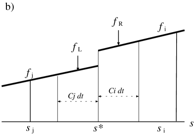
Figure 1: a) A schematic picture of the distribution of the function $f(s)$ in the vicinity of the $i$-th particle and the $j$-th. The value of the weighted average $f^{*}_{i,j}$ are determined by Eqs. (55), and its location $s^{*}_{i,j}$ by Eq. (56) or (64). b) The setup of Riemann problem. We define the piecewise linear distribution of physical variable $f(s)$ in both the $i$-th region and the $j$-th region. The initial values of each side of the one-dimensional Riemann problem are the average values in each domain of dependence.

Figure (1) shows schematic picture of the distribution of the function $f(s)$ in the vicinity of the $i$-th particle and the $j$-th. According to the original (grid-based) Godunov’s scheme, it is natural to define the interface of the two regions for the RP at $s^{*}_{i,j}$. To make the spatially second-order method like MUSCL, we define the piecewise linear distribution of physical variable $f(s)$ in both the $i$-th region and the $j$-th region. The gradient of $f(s)$ in each region can be simply assigned by the gradient at each particle’s position. The initial values on each side of one-dimensional Riemann problem is the average values of each domain of dependence, which is expressed as follows:

$$\rho_{R} = \rho_{i}+\left(\frac{\partial\rho}{\partial s}\right)_{i}\left[s^{*}_{i,j}+C_{{\rm s},i}\frac{\Delta t}{2}-s_{i}\right],$$

$$\ P_{R} = P_{i}+\left(\frac{\partial P}{\partial s}\right)_{i}\left[s^{*}_{i,j}+C_{{\rm s},i}\frac{\Delta t}{2}-s_{i}\right],$$

$$\ v_{R} = v_{i}+\left(\frac{\partial\ v}{\partial s}\right)_{i}\left[s^{*}_{i,j}+C_{{\rm s},i}\frac{\Delta t}{2}-s_{i}\right],$$

$$\rho_{L} = \rho_{j}+\left(\frac{\partial\rho}{\partial s}\right)_{j}\left[s^{*}_{i,j}-C_{{\rm s},j}\frac{\Delta t}{2}-s_{j}\right],$$

$$\ P_{L} = P_{j}+\left(\frac{\partial P}{\partial s}\right)_{j}\left[s^{*}_{i,j}-C_{{\rm s},j}\frac{\Delta t}{2}-s_{j}\right],$$

$$\ v_{L} = v_{j}+\left(\frac{\partial v}{\partial s}\right)_{j}\left[s^{*}_{i,j}-C_{{\rm s},j}\frac{\Delta t}{2}-s_{j}\right],$$ (67)

where

$$v_{i} = \mbox{\boldmath$v$}_{i}\cdot\mbox{\boldmath$e$}_{i,j},$$

$$v_{j} = \mbox{\boldmath$v$}_{j}\cdot\mbox{\boldmath$e$}_{i,j}.$$ (68)

and $C_{{\rm s},i}$ denotes the sound speed at $\mbox{\boldmath$x$}_{i}$. Thus we can solve the RP at the interface $s^{*}_{i,j}$. The detailed explanation for the solution of RP can be found in [24, 2], and we will not repeat it here.

After solving the RP at $s^{*}_{i,j}$, we have the resulting pressure $P^{*}_{i,j}$ and the projected velocity $v^{*}_{i,j}$. Three-dimensional (or two-dimensional) velocity $\mbox{\boldmath$v$}^{*}_{i,j}$ is calculated as follows:

$$\mbox{\boldmath$v$}^{*}_{i,j}=v^{*}_{i,j}\mbox{\boldmath$e$}_{i,j}+[\mbox{\boldmath$v$}_{i,j}-v_{i,j}\mbox{\boldmath$e$}_{i,j}],$$ (69)

where

$$\mbox{\boldmath$v$}_{i,j}=\mbox{\boldmath$v$}_{i}[1/2+\epsilon]+\mbox{\boldmath$v$}_{j}[1/2-\epsilon],$$ (70)

$$v_{i,j}=v_{i}[1/2+\epsilon]+v_{j}[1/2-\epsilon],$$ (71)

$$\epsilon=\frac{s^{*}_{i,j}}{\Delta s_{i,j}}.$$ (72)

These $P^{*}_{i,j}$ and $\mbox{\boldmath$v$}^{*}_{i,j}$ are used in the calculation of the right-hand side of Eqs. (65) and (66). Note that Eqs.(70), (71), (72) are not needed in the actual calculation, because the bracketed second term on the right-hand side of Eq. (69) is perpendicular to $\mbox{\boldmath$e$}_{i,j}$ and vanishes identically in Eq.(66).

In the higher-order grid-based methods (e.g., MUSCL and PPM) we need to impose monotonicity constraint on the gradients of physical variable to obtain the stable description of the discontinuity. This is also true in the present method. Our experience shows that the monotonicity constraint only on the velocity field suffices to make the stable method. Thus in the actual calculation of our method, we mimic the monotonicity constraints by setting

$$\left(\frac{\partial v}{\partial s}\right)_{i}=\left(\frac{\partial v}{\partial s}\right)_{j}=0~{}~{}~{}~{}{\rm if}~{}~{}~{}\left(\frac{\partial v}{\partial s}\right)_{i}\times\left(\frac{\partial v}{\partial s}\right)_{j}<0.$$ (73)

The numerical scheme should be first-order in space at the surface of the shock wave. The shock surface tends to include a few particles in the actual calculation. Therefore, if the velocity difference of a certain particle pair corresponds to the sound speed divided by a small number, the pair is considered to be in the shock surface, and we need to use the first-order Riemann Solver for this pair. We implement this condition by setting

$$\left(\frac{\partial f}{\partial s}\right)_{i}=\left(\frac{\partial f}{\partial s}\right)_{j}=0~{}~{}~{}{\rm if}~{}~{}C_{\rm shock}~{}\mbox{\boldmath$e$}_{i,j}\cdot(\mbox{\boldmath$v$}_{j}-\mbox{\boldmath$v$}_{i})>\min(C_{{\rm s},i},C_{{\rm s},j}),$$ (74)

where $f=\rho,~{}P,~{}v$, and $C_{\rm shock}$ is a numerical constant corresponding to the number of particles at the shock surface. We adopt $C_{\rm shock}=3$ throughout in this paper.

3.3 Variable Smoothing Length

In the previous subsections, we assume that the smoothing length, $h$, is constant in space. In actual calculation we need to change $h$ to enlarge the dynamic range of the spatial resolution. Therefore we have to extend the present method for the variable smoothing length.

The formal derivation of the evolution equation with variable smoothing length is the same as Section 2.2, except that we should start with the definition of density as

$$\rho(\mbox{\boldmath$x$})=\sum_{j}m_{j}W(\mbox{\boldmath$x$}-\mbox{\boldmath$x$}_{j},h[\mbox{\boldmath$x$}]).$$ (75)

This definition of density corresponds to the so-called “gather” formulation of SPH [8]. The resulting evolution equations are the following:

$$\ddot{\mbox{\boldmath$x$}}_{i} = \sum_{j}m_{j}P^{*}_{i,j}\int\frac{1}{\rho^{2}(\mbox{\boldmath$x$})}\left\{\nabla W(\mbox{\boldmath$x$}-\mbox{\boldmath$x$}_{i},h[\mbox{\boldmath$x$}])W(\mbox{\boldmath$x$}-\mbox{\boldmath$x$}_{j},h[\mbox{\boldmath$x$}])\right.$$ (76)

$$~{}~{}~{}~{}~{}~{}~{}~{}~{}~{}~{}~{}~{}~{}~{}~{}~{}~{}~{}~{}~{}~{}~{}~{}~{}~{}~{}\left.-W(\mbox{\boldmath$x$}-\mbox{\boldmath$x$}_{i},h[\mbox{\boldmath$x$}])\nabla W(\mbox{\boldmath$x$}-\mbox{\boldmath$x$}_{j},h[\mbox{\boldmath$x$}])\right\}d\mbox{\boldmath$x$},$$

$$\dot{u}_{i} = \sum_{j}m_{j}P^{*}_{i,j}(\mbox{\boldmath$v$}^{*}_{i,j}-\mbox{\boldmath$v$}_{i})\int\frac{1}{\rho^{2}(\mbox{\boldmath$x$})}\left\{\nabla W(\mbox{\boldmath$x$}-\mbox{\boldmath$x$}_{i},h[\mbox{\boldmath$x$}])W(\mbox{\boldmath$x$}-\mbox{\boldmath$x$}_{j},h[\mbox{\boldmath$x$}])\right.$$ (77)

$$~{}~{}~{}~{}~{}~{}~{}~{}~{}~{}~{}~{}~{}~{}~{}~{}~{}~{}~{}~{}~{}~{}~{}~{}~{}~{}~{}~{}~{}\left.-W(\mbox{\boldmath$x$}-\mbox{\boldmath$x$}_{i},h[\mbox{\boldmath$x$}])\nabla W(\mbox{\boldmath$x$}-\mbox{\boldmath$x$}_{j},h[\mbox{\boldmath$x$}])\right\}d\mbox{\boldmath$x$}.$$

These equations are essentially the same as Eqs. (65) and (66), although the analytic integration for these equation is not possible even with the polynomial approximation for $\rho^{-2}(\mbox{\boldmath$x$})$. Therefore we prefer to use simple approximation for the integral as in the following form:

$$\frac{\Delta\dot{\mbox{\boldmath$x$}}_{i}}{\Delta t} = -\sum_{j}m_{j}P^{*}\left[~{}V^{2}_{i,j}(h_{i})\frac{\partial}{\partial\mbox{\boldmath$x$}_{i}}W(\mbox{\boldmath$x$}_{i}-\mbox{\boldmath$x$}_{j},\sqrt{2}h_{i})\right.$$ (78)

$$~{}~{}~{}~{}~{}~{}~{}~{}~{}~{}~{}~{}~{}~{}~{}~{}~{}~{}~{}\left.+V^{2}_{i,j}(h_{j})\frac{\partial}{\partial\mbox{\boldmath$x$}_{i}}W(\mbox{\boldmath$x$}_{i}-\mbox{\boldmath$x$}_{j},\sqrt{2}h_{j})~{}\right],$$

$$\frac{\Delta u_{i}}{\Delta t} = -\sum_{j}m_{j}[P^{*}\mbox{\boldmath$v$}^{*}-P^{*}\dot{\mbox{\boldmath$x$}}_{i}^{*}]\left[~{}V^{2}_{i,j}(h_{i})\frac{\partial}{\partial\mbox{\boldmath$x$}_{i}}W(\mbox{\boldmath$x$}_{i}-\mbox{\boldmath$x$}_{j},\sqrt{2}h_{i})\right.$$ (79)

$$~{}~{}~{}~{}~{}~{}~{}~{}~{}~{}~{}~{}~{}~{}~{}~{}~{}~{}~{}~{}~{}~{}~{}~{}~{}~{}~{}~{}~{}~{}~{}\left.+V^{2}_{i,j}(h_{j})\frac{\partial}{\partial\mbox{\boldmath$x$}_{i}}W(\mbox{\boldmath$x$}_{i}-\mbox{\boldmath$x$}_{j},\sqrt{2}h_{j})~{}\right],$$

where, in spirit, we used $h_{i}$ for the half of the integration space which include $\mbox{\boldmath$x$}_{i}$, and used $h_{j}$ for the other half.

The above approximations assume that the $h(\mbox{\boldmath$x$})$ should not vary much within the neighborhood of each particle. One possible way to determine the smoothing length with this constraint is the following:

$$h_{i}=\eta\left[\frac{m_{i}}{\rho^{*}_{i}}\right]^{1/d},$$ (80)

where

$$\rho^{*}_{i}=\sum_{j}m_{j}W(\mbox{\boldmath$x$}_{i}-\mbox{\boldmath$x$}_{j},h^{*}_{i}),~{}~{}~{}h^{*}_{i}=h_{i}C_{\rm smooth}.$$ (81)

$\rho^{*}$ is more smooth than $\rho$ itself if $C_{\rm smooth}>1$ . Numerical experiments shows that $\eta\simeq 1$ with $C_{\rm smooth}\simeq 2$ works fine in Section 4. The effective number of neighbors around each particle depends on the ratio of the smoothing length and the mean separation of particles at that particle. For example, we can usually ignore the contribution from the $j$-th particle to the $i$-th particle if their distance $|\mbox{\boldmath$x$}_{i}-\mbox{\boldmath$x$}_{j}|$ is larger than $3h_{i}$, because $\exp(-3^{2})\approx 1.234\times 10^{-4}$. Thus, in one-dimensional calculations, the number of neighbors for calculating Eq.(81) is $6\eta C_{\rm smooth}$ excluding the $i$-th particle itself. The number of neighbors becomes about $28\eta^{2}C_{\rm smooth}^{2}$ in two-dimensional calculations, and about $113\eta^{3}C_{\rm smooth}^{3}$ in three dimensional calculations.

3.4 Conservation Property

The final discretized form for the equation of motion for the $i$-th particle becomes the following:

$$\Delta\dot{\mbox{\boldmath$x$}}_{i} = -\Delta t\sum_{j}m_{j}P^{*}_{i,j}\left[V^{2}_{i,j}(h_{i})\frac{\partial}{\partial\mbox{\boldmath$x$}_{i}}W(\mbox{\boldmath$x$}_{i}-\mbox{\boldmath$x$}_{j},\sqrt{2}h_{i})\right.$$ (82)

$$~{}~{}~{}~{}~{}~{}~{}~{}~{}~{}~{}~{}~{}~{}~{}~{}~{}~{}~{}~{}~{}~{}~{}~{}~{}~{}~{}~{}~{}\left.+V^{2}_{i,j}(h_{j})\frac{\partial}{\partial\mbox{\boldmath$x$}_{i}}W(\mbox{\boldmath$x$}_{i}-\mbox{\boldmath$x$}_{j},\sqrt{2}h_{j}).\right]$$

This calculation guarantees the conservation of the total momentum of the system,

$$\sum_{i}m_{i}\Delta\dot{\mbox{\boldmath$x$}}_{i}=0,$$ (83)

because the terms in the square bracket in Eq. (82) are anti-symmetric in $i$ and $j$.

The final form for the equation of energy for the $i$-th particle becomes the following:

$$\Delta u_{i} = -\Delta t\sum_{j}m_{j}P^{*}_{i,j}(\mbox{\boldmath$v$}^{*}_{i,j}-\dot{\mbox{\boldmath$x$}}^{*}_{i})\left[V^{2}_{i,j}(h_{i})\frac{\partial}{\partial\mbox{\boldmath$x$}_{i}}W(\mbox{\boldmath$x$}_{i}-\mbox{\boldmath$x$}_{j},\sqrt{2}h_{i})\right.$$ (84)

$$~{}~{}~{}~{}~{}~{}~{}~{}~{}~{}~{}~{}~{}~{}~{}~{}~{}~{}~{}~{}~{}~{}~{}~{}~{}~{}~{}~{}~{}~{}~{}~{}~{}~{}~{}~{}\left.+V^{2}_{i,j}(h_{j})\frac{\partial}{\partial\mbox{\boldmath$x$}_{i}}W(\mbox{\boldmath$x$}_{i}-\mbox{\boldmath$x$}_{j},\sqrt{2}h_{j})\right]$$

where we defined the time-centered velocity of the $i$-th particle,

$$\dot{\mbox{\boldmath$x$}}^{*}_{i}=\dot{\mbox{\boldmath$x$}}_{i}+\frac{1}{2}\Delta\dot{\mbox{\boldmath$x$}}_{i}.$$ (85)

This expression guarantees the conservation of the total energy of the system, because

$$\Delta\sum_{i}m_{i}\left[\frac{1}{2}\mbox{\boldmath$\dot{x}$}_{i}^{2}+u_{i}\right]$$ (86)

$$= \sum_{i}m_{i}\left\{\frac{1}{2}[\mbox{\boldmath$\dot{x}$}_{i}+\Delta\mbox{\boldmath$\dot{x}$}_{i}]^{2}+[u_{i}+\Delta u_{i}]-\frac{1}{2}\mbox{\boldmath$\dot{x}$}_{i}^{2}-u_{i}\right\}$$

$$= \sum_{i}m_{i}\left\{\Delta\mbox{\boldmath$\dot{x}$}_{i}\left[\mbox{\boldmath$\dot{x}$}_{i}+\frac{1}{2}\Delta\mbox{\boldmath$\dot{x}$}_{i}\right]+\Delta u_{i}\right\}$$

$$= -\sum_{i}\sum_{j}m_{i}m_{j}P^{*}_{i,j}\mbox{\boldmath$v$}^{*}_{i,j}\left[V^{2}_{i,j}(h_{i})\frac{\partial}{\partial\mbox{\boldmath$x$}_{i}}W(\mbox{\boldmath$x$}_{i}-\mbox{\boldmath$x$}_{j},\sqrt{2}h_{i})\right.$$

$$~{}~{}~{}~{}~{}~{}~{}~{}~{}~{}~{}~{}~{}~{}~{}~{}~{}~{}~{}~{}~{}~{}~{}~{}~{}~{}~{}~{}~{}~{}~{}~{}\left.+V^{2}_{i,j}(h_{j})\frac{\partial}{\partial\mbox{\boldmath$x$}_{i}}W(\mbox{\boldmath$x$}_{i}-\mbox{\boldmath$x$}_{j},\sqrt{2}h_{j})\right]$$

$$= 0.$$

Thus the present scheme conserves energy exactly. This is in contrast to the ordinary energy equation of the standard SPH which is only accurate in the first-order in time (see, e.g., [1, 18]). We also note that the conservation of energy does not require constant smoothing length, which is obvious in Eq. (86). This is because the expression of the total energy in the numerical calculation $\sum_{i}m_{i}(\frac{1}{2}\mbox{\boldmath$x$}_{i}^{2}+u_{i})$ does not explicitly depends on the choice of smoothing length. In other words, a sudden change of smoothing length at any timestep does not change the numerical value of the total energy.

3.5 Overall Procedure

In this section we summarize the actual procedures in the sequence of executions. The main loop of the time integration corresponds to Steps 1-4.

Step 0. Problem Setup
      We first setup the problem in the computer program. We appropriately place the particles to represent the density distribution that corresponds to the initial condition of the problem to solve. This may require some relaxation technique to find the appropriate positions of the particles [18]. We also determine $\rho_{i}$, $\nabla\rho_{i}$, and $h_{i}$ to start the main loop of the time integration. Various constants and the initial variables are calculated in this step. For example we determine the initial timestep $\Delta t$.

Step 1. Gradient Calculation
      We calculate the gradient of physical variables $P,\mbox{\boldmath$v$}$ for the use in the Riemann Solver.

Step 2. Source Term Calculation
      We calculate the RHS of Eqs.(82),(84) either by Eq.(52) or Eq.(63). The subroutine for the Riemann Solver is called once for every pair of particles to calculate $P^{*}$ and $v^{*}$ in Eqs.(82),(84).

Step 3. Time Evolution
      We update $\mbox{\boldmath$x$}_{i}$, $\mbox{\boldmath$\dot{x}$}_{i}$, and $u_{i}$ according to Eqs.(85),(82),(84) ,

$$\mbox{\boldmath$x$}_{i}(t+\Delta t) = \mbox{\boldmath$x$}_{i}(t)+\dot{\mbox{\boldmath$x$}}_{i}^{*}\Delta t,$$

$$\dot{\mbox{\boldmath$x$}}_{i}(t+\Delta t) = \dot{\mbox{\boldmath$x$}}_{i}(t)+\Delta\dot{\mbox{\boldmath$x$}}_{i},$$

$$u_{i}(t+\Delta t) = u_{i}(t)+\Delta u_{i}.$$ (87)

Step 4. Density Updation
      According to the updated positions of particles, we update density distribution. The smoothing length of each particle is also updated. The timestep $\Delta t$ for the next integration is also determined. We turn to Step 1 for the next time integration.

4 Numerical Examples

The present method was tested on a variety of 1D, 2D, and 3D problems, a few of which are described below. Other sets of test calculations will be described elsewhere.

In determining the amount of the timestep $\Delta t$, we have to consider the Courant condition that is in spirit similar to the Courant condition for the grid-based Lagrangian methods,

$$\Delta t=C_{\rm CFL}\min_{i}\left\{\left.\left[\frac{m_{i}}{\rho_{i}}\right]^{1/d}\right/C_{{\rm s},i}\right\}.$$ (88)

The numerical experiments show that we can safely use $C_{\rm CFL}\approx 0.5$ in most of hydrodynamical problems. Note that we don’t need to consider the (effective) diffusion timescale that is related to the artificial viscosity adopted by the standard SPH and other particle methods. Thus $\Delta t$ in the present method can be much larger than that in the other SPH methods.

The following examples are calculated with the Fortran program in which the single precision real number is used. To accelerate the computation we use the data structure based on link lists [16].

Five cycles of iterations in the Riemann Solver is sufficient for the following test problems.

4.1 Shock Tube

Figure 2: Results of the shock tube problem in which the Mach number is 1.526. The right-hand side of the initial discontinuity includes 40 equal-mass particles. The open circles plot the snapshot at $t=0.2$ by the present method with the cubic spline approximation for the convolution Eq.(63) and the variable smoothing length ($\eta=1$, $C_{\rm smooth}=2.0$). The solid lines correspond to the analytic solution.

In order to compare the capabilities of the present method and standard SPH we test our method against the shock tube problems, of which the exact solutions are available. The density variation in the first problem is not so large that we can use both the variable smoothing length and the constant smoothing length. The initial parameters of the problem are the following:

$$\rho_{\rm L}=1 ,~{}~{}~{} \rho_{\rm R}=0.5,$$

$$P_{\rm L}=1 ,~{}~{}~{} P_{\rm R}=0.2,$$

$$v_{x,{\rm L}}=0 ,~{}~{}~{} v_{x,{\rm R}}=0,$$ (89)

where the subscript “L” denotes the variable on the left-hand side of the initial discontinuity, and R denotes the right-hand side. The ratio of specific heats is $\gamma=7/5$. The Mach number of the resultant shock wave is $1.526$. The value of the post-shock pressure is $P^{*}=0.5099$. Figure 2 plots the snapshot at $t=0.2$ by the present method with the cubic spline approximation for the convolution Eq.(63) and the variable smoothing length ($\eta=1$, $C_{\rm smooth}=2.0$). The method with the linear approximation for the convolution Eq.(52) gives very similar result. Figure 3 plots the corresponding result of the standard SPH where we used the “standard” artificial viscosity ($\alpha=1,\beta=2$) described in the review paper by Monaghan [18]. In both cases, the number of equal-mass particles is 80 (40) on the left(right)-hand side of initial discontinuity (i.e., $\Delta x_{L}=0.005$, $\Delta x_{R}=0.01$ ). The solid lines correspond to the analytic solution. In this problem, these two methods give similar results except for the contact discontinuity where the standard SPH produced a “wiggle” in pressure and specific internal energy. This is due to the inconsistency of EoM of the standard SPH (45). The present method produced the smooth distribution of internal energy at the contact discontinuity, and hence provide the almost constant pressure distribution at the density discontinuity.

The total energy of the system ($-0.4<x<0.4$) is defined as

$$\int_{-0.4}^{0.4}\frac{1}{2}\rho u~{}dx=1.2.$$ (90)

The initial numerical value of the total energy of the particle system was the following:

$$\sum_{i}m_{i}u_{i}=1.20000017$$ (91)

where the last few digits have no significant meaning in this Fortran single precision calculation. The final ($t=0.2$) value of the total energy of the particle system was found to be

$$\sum_{i}m_{i}(\frac{1}{2}\dot{\mbox{\boldmath$x$}}_{i}^{2}+u_{i})=1.20003033$$ (92)

The relative error remains sufficiently small ($\Delta E/E<10^{-4}$) when we change $\Delta t$ in the other runs. Thus the error of the total energy is only due to the round-off error of the single precision calculation, and not due to the truncation errors in the numerical modeling of the evolution. This result guarantees the strict conservation property of the present scheme (see Section 3.4).

The present method spent 0.17 seconds for the total 52 timesteps ($\Delta t\approx 0.004$) to compute with the Hewlett-Packard workstation C240 (PA-RISC 8200/236MHz), which corresponds to $3.27\times 10^{-3}$ seconds per step and $2.72\times 10^{-5}$ seconds per particle. In contrast the standard SPH method used 956 timesteps ($\Delta t\approx 0.0002$) for the stable evolution in this problem, because the artificial viscosity limits $\Delta t$. Indeed numerical experiments shows larger $\Delta t$ causes unphysical oscillations in the solution. As a result the standard SPH method spent 1.35 seconds to finish the calculation. It corresponds to $1.4\times 10^{-3}$ seconds per step and $1.2\times 10^{-5}$ seconds per particle. This means that the present method is about two times slower than the standard SPH for the required operations per particle but the present method tends to spend much smaller (total) computation time than the standard SPH does.

Figure 4 plot the result of the present method where we used the constant smoothing length $h=0.01$. The rarefaction wave on the left hand side is described less-accurately than in Fig. 2 as expected, because the smoothing length in high density region in Fig. 2 is smaller than the constant smoothing length in Fig. 4. The method with the constant smoothing length has no advantage over the method with the variable smoothing length even in this kind of shock tube problem where the density variation is not so large.

Figure 5 plot the result of the present method with the first-order Riemann Solver where we set $\partial\rho/\partial s=\partial P/\partial s=\partial v/\partial s=0$ in the Riemann Solver. The sharp profiles at the shock front and the head and tail of the rarefaction wave are smeared out as in the grid-based first-order Godunov method. In this calculation we don’t need to calculate the gradients of $P$ and $v_{x}$. However the difference of the computation times with the first- and second-order method is negligible. There is no reason to use this first-order method.

Figure 3: Results of the shock tube problem in which the Mach number is 1.526. The open circles plot the snapshot at $t=0.2$ by the standard SPH. The solid lines correspond to the analytic solution.

Figure 4: Same as Fig. 2 except that we used the constant smoothing length $h=0.01$.

Figure 5: Same as Fig. 2 except that we used the first-order Riemann Solver.

In Fig. 6, the results of the standard Sod’s shock tube [23] are plotted. The initial parameters of the problem are the following:

$$\rho_{\rm L}=1 \rho_{\rm R}=0.125,$$ ,

$$P_{\rm L}=1 P_{\rm R}=0.1,$$ ,

$$v_{x,{\rm L}}=0 v_{x,{\rm R}}=0.$$ , (93)

The ratio of specific heats is $\gamma=7/5$. The solid lines correspond to the analytic solution. The number of the equal-mass particles in the $x$-direction is 40 on the right-hand side of the initial discontinuity. We used the variable smoothing length ($\eta=1$, $C_{\rm smooth}=2.0$).

Figure 6: Results of the Sod’s shock tube problem by the present method with the cubic spline approximation for the convolution Eq.(63) and the variable smoothing length ($\eta=1$, $C_{\rm smooth}=2.0$). The solid lines correspond to the analytic solution.

4.2 Extreme Blast Wave

Figure 7: Results of 1D calculation for the extremely strong shock tube problem of which Mach number is about $10^{5}$. We used 100 particles on each side of the initial discontinuity. The open circles plot the result of the present method where the cubic spline approximation for the convolution Eq.(63) and the variable smoothing length are used ($\eta=1$, $C_{\rm smooth}=2.0$). A small wiggle in the pressure distribution at the contact surface is due to the approximation for the convolution.

Figure 8: Same as Fig.7 except that we used the linear interpolation in the convolution Eq.(52). The amplitude of the pressure wiggling at the contact surface is slightly larger than that of the cubic spline result.

To explore the capability of the present method, we test our method against an extremely strong shock tube problem. The initial parameters of the problem are the following:

$$\rho_{\rm L}=1 \rho_{\rm R}=1,$$ ,

$$P_{\rm L}=3000 P_{\rm R}=10^{-7},$$ ,

$$v_{x,{\rm L}}=0 v_{x,{\rm R}}=0,$$ , (94)

where the initial pressure of the gas on the left-hand side is $3\times 10^{10}$ times that of the right-hand side. The ratio of specific heats is $\gamma=5/3$. The Mach number is as large as $10^{5}$. We used 100 particles on each side of the initial discontinuity. Figure 7 plots the result of the present method where the cubic spline approximation for the convolution Eq.(63) and the variable smoothing length is used ($\eta=1$, $C_{\rm smooth}=2.0$). Even in this severe problem, the present method gave stable and accurate results and is free from penetration problems. The pressure distribution shows a small wiggle at the contact surface. This is due to the approximation for the convolution. Figure 8 plots the result of the present method with the linear interpolation Eq.(52). The amplitude of the pressure wiggling at the contact surface is slightly larger than that of the cubic spline result. In order to eliminate this unphysical wiggling, we need to develop more accurate approximation for the numerical convolution than Eq.(63). Numerical experiments shows that the standard SPH cannot produce acceptable result at least with $\eta=1$, $\alpha\approx 1$, and $\beta\approx 2$. The possible fine-tuning of the parameters in the standard SPH may enable the calculation in this case. Note that the present method can describe this extreme phenomena with the same parameters ($\eta=1$, $C_{\rm smooth}=2.0$) used in the other test problems, without any tuning of the method.

The accurate calculation with the single precision real numbers in the Fortran program is due to the conservative formulation with the internal specific energy $u$ instead of the total energy $e$ ($=v^{2}/2+u$) or $E$ ($=\rho v^{2}/2+\rho u$) which are usually used in the grid-based conservative numerical schemes (see Section 3.4). If we adopt $e$ or $E$ as the main variable for the integration, we have to do the subtraction to obtain $u$ ($=e-v^{2}/2$), which brings huge error into the numerical value of $u$ in the extremely supersonic motion (i.e., when $u\ll e\approx v^{2}/2$). In this sense our method has potential advantage over the grid-based higher-order Godunov methods, at least, in describing extremely supersonic flows.

4.3 Wind-Tunnel

To test the present method against multi-dimensional problem, we adopt the following wind-tunnel problem [12], that can be in principle directly compared with the laboratory experiment. The geometry is a two-dimensional channel with a $15^{\circ}$ wedge on the lower wall. A $15^{\circ}$ expansion corner is also included. The inflow Mach number is two. This kind of problem is poorly suited for the particle method because a rigid-wall boundary condition must be set up at the wall of the tunnel. We present this test problem only to demonstrate the capability of our scheme.

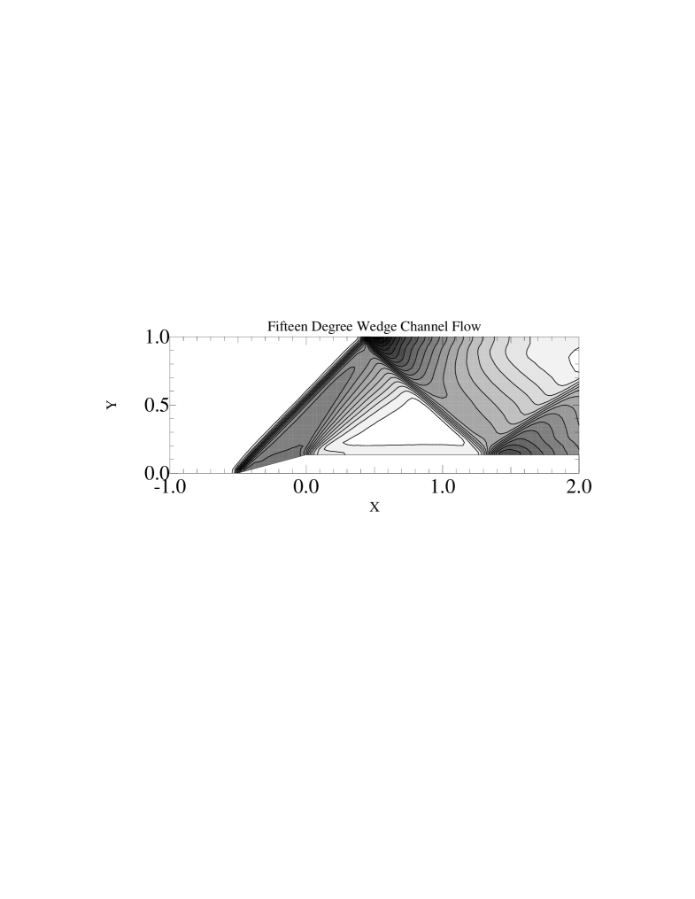
Figure 9: Results of calculation on “fifteen degree wedge channel flow” problem. Initially 32$\times$96 particles are flowing inside the channel. Mach-number contours from 0.92 to 1.97 with an increment of 0.05 are plotted.

Figure 10: Same as Fig.9 but positions of particles are plotted. The crosses denote the positions of “ghost particles” that are introduced to mimic the rigid wall boundary condition.

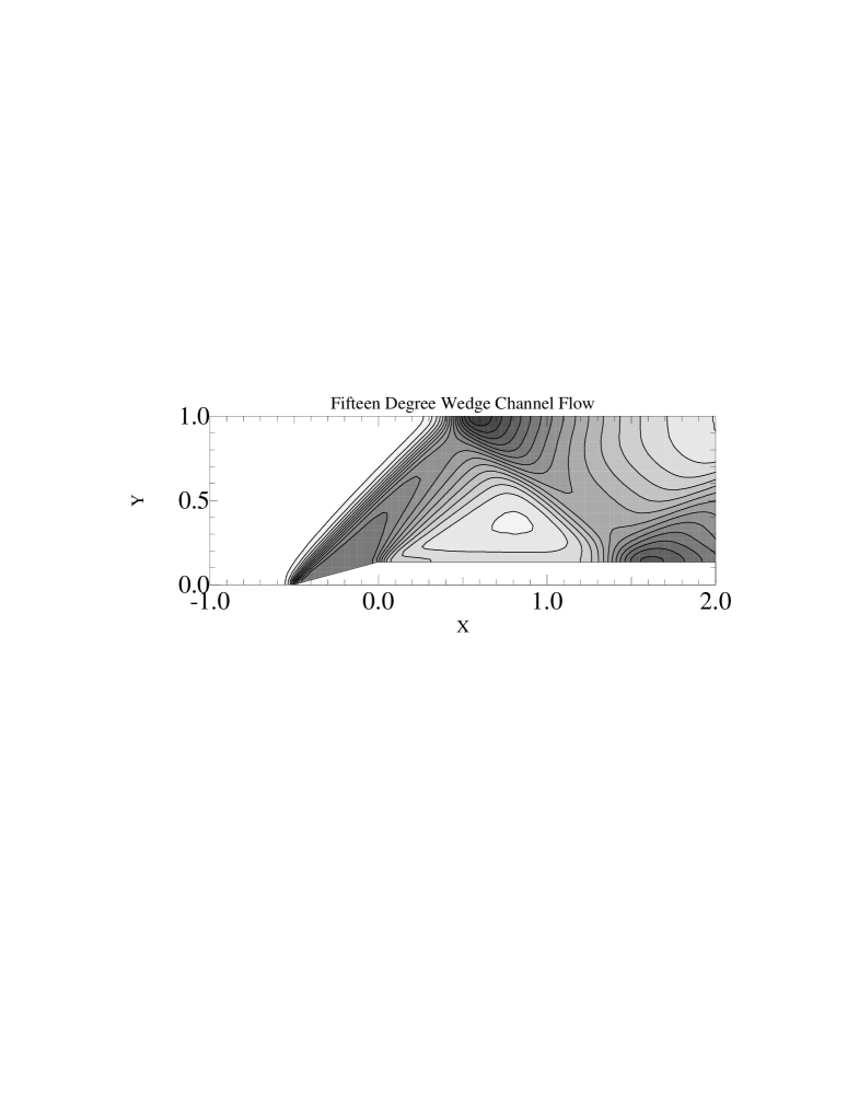
Figure 11: Results of calculation on “fifteen degree wedge channel flow” problem with the first-order Riemann Solver. Initially 32$\times$96 particles are flowing inside the channel. The contour levels are the same as Fig.9.

Figure 12: Results of calculation on “fifteen degree wedge channel flow” problem with the standard SPH. The standard artificial viscosity with $\alpha=1,\beta=2$ are used. Initially 32$\times$96 particles are flowing inside the channel. The contour levels are the same as Fig.9.

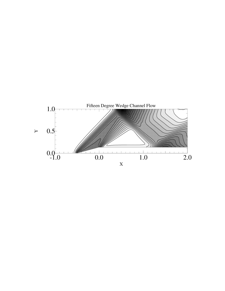
Figure 13: Results of calculation on “fifteen degree wedge channel flow” problem with the standard SPH. The standard artificial viscosity with $\alpha=2,\beta=4$ are used. Initially 32$\times$96 particles are flowing inside the channel. The contour levels are the same as Fig.9.

Figure 9 shows our method’s result. Mach-number contours from 0.92 to 1.97 with an increment of 0.05 are plotted. Figure 10 shows particle positions. In this calculation, we realized the rigid-wall boundary condition by placing “ghost particles” in the wall. The inflowing particles outside of the left-hand side boundary were prepared at appropriate timesteps. The variable smoothing length is used ($\eta=1$, $C_{\rm smooth}=1.0$). Initially, 32$\times$96 particles were flowing inside the channel, which may be compared to the 32$\times$96 grids finite difference calculation in [12]. Our results were satisfactory. For comparison, Figure 11 shows the result for the first-order Riemann Solver. The sharp features are smeared out.

Figure 12 shows results of calculation with the standard SPH, where the standard artificial viscosity with $\alpha=1,\beta=2$ are used. Note that the contour levels are the same as Fig. 9. Owing to the moderate strength of the shocks in this problem, the standard SPH could produce reasonable result except for the region just after the Mach stem on the upper wall. A small hollow semicircle seen at $x\approx 0.5$, $y\approx 1$ corresponds to the small value of Mach number ($=0.806$) that is caused by an exceedingly large value of the post shock pressure. The calculations with larger values of the artificial viscosity parameters tend to remedy this pressure overshooting. Figure 13 shows the result of the standard SPH with $\alpha=2,\beta=4$ where the minimum value of Mach number behind the Mach stem is 0.957. In this case, however, the sharp features are smeared out. Even in this two dimensional problem of moderate Mach number, the present method shows its potential ability in analyzing supersonic flows.

It is clear that a grid-based method must be used in the actual study of this kind of steady rigid-wall boundary problem. This result is presented only to demonstrate the capability of this particle scheme. The present method becomes more useful when we study the hydrodynamical problems without rigid boundary that are common in astrophysics and space sciences.

5 Summary

Smoothed Particle Hydrodynamics is reformulated by the formal convolution of the original hydrodynamics equations, and by a new action principle, in which the second order (in $h$) approximation is used for the kinetic term of the Lagrangian function. The force acting on each particle is determined by solving the Riemann problem for each particle pair. The prescription for variable smoothing length is also shown. These techniques are implemented in the strict conservation form. Numerical examples involving an extremely strong shock are shown. The other test calculations will be described elsewhere.

Although the method with a spatially constant smoothing length is formulated in a rigorous manner, the method with the variable smoothing length is based on a crude approximation (Eqs. [78],[79]). A more refined technique for the variable smoothing length is to be studied. A better approximation than the cubic spline interpolation in the numerical convolution is required to eliminate the “wiggle” at the contact discontinuity in the blast wave problems (see Section 4.2).

This paper presented a piece of concepts that are not discussed in detail in the literature. Those are the convolution of the original fluid equation (Eqs. [20],[24]), the definition and approximation for the velocity field (Eqs. [34], [39]), and the modification of the force due to dissipation (Eqs. [65], [66]). Incorporating these concept, the final evolution equation was cast into a form similar to the standard SPH equation. Therefore those concepts may enable the rigorous examination of the accuracy and stability of the method and may enable further modification.

The numerical examples in Section 4 show that the present particle method based on Riemann Solver can handle severe problems with strong shocks, those might include the description of explosion/implosion and supersonic jet phenomena. In this respect, further modification of the SPH method in modeling relativistic flows is promising with the help of relativistic Riemann Solver [15]. In adittion, the Lagrangian particle methods have advantage over Eulerian grid-based methods, in describing chemically reacting (multi)fluid and radiatively heating/cooling fluid [11]. This is because we can simply assign the chemical composition and entropy to each particle as a fluid element. This direction has a wide area of applications.

The author thanks the anonymous referee for valuable comments. The author also thanks Toru Tsuribe, Yusuke Imaeda, and Shoken M. Miyama for useful discussions.

Appendix A Derivation of the Equation of Motion

In this Appendix we show the derivation of the equation of motion from the Euler-Lagrange’s equation (Eq.[42]).

$$\frac{\partial L}{\partial\mbox{\boldmath$x$}_{i}} = -\sum_{k}m_{k}\int\frac{\partial u}{\partial\mbox{\boldmath$x$}_{i}}W(\mbox{\boldmath$x$}-\mbox{\boldmath$x$}_{k},h)d\mbox{\boldmath$x$}$$ (95)

$$-m_{i}\int u\frac{\partial}{\partial\mbox{\boldmath$x$}_{i}}W(\mbox{\boldmath$x$}-\mbox{\boldmath$x$}_{i},h)d\mbox{\boldmath$x$}.$$

The first term on the RHS of this equation becomes the following:

$$-\sum_{k}m_{k}\int\frac{\partial u}{\partial\mbox{\boldmath$x$}_{i}}W(\mbox{\boldmath$x$}-\mbox{\boldmath$x$}_{k},h)d\mbox{\boldmath$x$}$$ (96)

$$= -\sum_{k}m_{k}\int\frac{P}{\rho^{2}}\frac{\partial\rho}{\partial\mbox{\boldmath$x$}_{i}}W(\mbox{\boldmath$x$}-\mbox{\boldmath$x$}_{k},h)d\mbox{\boldmath$x$}$$

$$= -\sum_{k}m_{k}\int\frac{P}{\rho^{2}}m_{i}\frac{\partial W(\mbox{\boldmath$x$}-\mbox{\boldmath$x$}_{i},h)}{\partial\mbox{\boldmath$x$}_{i}}W(\mbox{\boldmath$x$}-\mbox{\boldmath$x$}_{k},h)d\mbox{\boldmath$x$}.$$

Before we manipulate the second term on the RHS of Eq. (95), we note that

$$\frac{\partial W(\mbox{\boldmath$x$}-\mbox{\boldmath$x$}_{i},h)}{\partial\mbox{\boldmath$x$}_{i}}=-\frac{\partial W(\mbox{\boldmath$x$}-\mbox{\boldmath$x$}_{i},h)}{\partial\mbox{\boldmath$x$}}.$$ (97)

We also obtain

$$\int f(\mbox{\boldmath$x$})\frac{\partial W(\mbox{\boldmath$x$}-\mbox{\boldmath$x$}_{i},h)}{\partial\mbox{\boldmath$x$}}d\mbox{\boldmath$x$}=-\int\frac{\partial f(\mbox{\boldmath$x$})}{\partial\mbox{\boldmath$x$}}W(\mbox{\boldmath$x$}-\mbox{\boldmath$x$}_{i},h)d\mbox{\boldmath$x$},$$ (98)

by the integration by parts and $W(\mbox{\boldmath$x$})\rightarrow 0~{}~{}(|\mbox{\boldmath$x$}|\rightarrow\infty)$ .

Using the above identities, we can transform the second term on the RHS of Eq. (95) as

$$-m_{i}\int u\frac{\partial}{\partial\mbox{\boldmath$x$}_{i}}W(\mbox{\boldmath$x$}-\mbox{\boldmath$x$}_{i},h)d\mbox{\boldmath$x$}$$ (99)

$$= +m_{i}\int u\frac{\partial}{\partial\mbox{\boldmath$x$}}W(\mbox{\boldmath$x$}-\mbox{\boldmath$x$}_{i},h)d\mbox{\boldmath$x$}$$

$$= -m_{i}\int\frac{\partial u}{\partial\mbox{\boldmath$x$}}W(\mbox{\boldmath$x$}-\mbox{\boldmath$x$}_{i},h)d\mbox{\boldmath$x$}$$

$$= -m_{i}\int\frac{P}{\rho^{2}}\frac{\partial\rho}{\partial\mbox{\boldmath$x$}}W(\mbox{\boldmath$x$}-\mbox{\boldmath$x$}_{i},h)d\mbox{\boldmath$x$}$$

$$= -m_{i}\int\frac{P}{\rho^{2}}\sum_{j}m_{j}\frac{\partial W(\mbox{\boldmath$x$}-\mbox{\boldmath$x$}_{j},h)}{\partial\mbox{\boldmath$x$}}W(\mbox{\boldmath$x$}-\mbox{\boldmath$x$}_{i},h)d\mbox{\boldmath$x$}$$

$$= m_{i}\int\frac{P}{\rho^{2}}\sum_{j}m_{j}\frac{\partial W(\mbox{\boldmath$x$}-\mbox{\boldmath$x$}_{j},h)}{\partial\mbox{\boldmath$x$}_{j}}W(\mbox{\boldmath$x$}-\mbox{\boldmath$x$}_{i},h)d\mbox{\boldmath$x$}.$$

As a result, Euler-Lagrange’s equation gives the following:

$$\ddot{\mbox{\boldmath$x$}}_{i} = -\sum_{j}m_{j}\int\frac{P}{\rho^{2}}\frac{\partial}{\partial\mbox{\boldmath$x$}_{i}}W(\mbox{\boldmath$x$}-\mbox{\boldmath$x$}_{i},h)W(\mbox{\boldmath$x$}-\mbox{\boldmath$x$}_{j},h)d\mbox{\boldmath$x$}$$ (100)

$$+\sum_{j}m_{j}\int\frac{P}{\rho^{2}}\frac{\partial}{\partial\mbox{\boldmath$x$}_{j}}W(\mbox{\boldmath$x$}-\mbox{\boldmath$x$}_{i},h)W(\mbox{\boldmath$x$}-\mbox{\boldmath$x$}_{j},h)d\mbox{\boldmath$x$}.$$

References

• [1] W. Benz, Smooth Particle Hydrodynamics - a Review, in Proc Numerical Modelling of Nonlinear Stellar Pulsations: Problems and Prospects, Les Arcs, France, March 1989, edited by J. Robert Buchler, (Kluwer, Dordrecht/Boston, 1990), P.269.
• [2] P. Colella and P. Woodward, Piecewise Parabolic Method (PPM) for Gas-Dynamical Simulations, J. Computat. Phys. 54, 174 (1984)
• [3] G. A. Dilts, Moving-Least-Squares-Particle Hydrodynamics –I. Consistency and Stability, Int. J. Numer. Meth. Engng. 44, 1115 (1999)
• [4] G. A. Dilts, Moving-Least-Squares-Particle Hydrodynamics –II. Conservation and Boundaries, Int. J. Numer. Meth. Engng. 48, 1503 (2000)
• [5] D. A. Fulk and D. W. Quinn, Hybrid Formulations of Smoothed Particle Hydrodynamics, Int. J. Impact Engng. 17, 329 (1995)
• [6] S. K. Godunov, Difference Methods for the Numerical Calculation of the Equations of Fluid Dynamics, Mat. Sb. 47, 271 (1959)
• [7] R. A. Gingold and J. J. Monaghan, Smoothed Particle Hydrodynamics – Theory and Application to Non-Spherical Stars, Mon. Not. R. Astron. Soc. 181, 375 (1977)
• [8] L. Hernquist & N. Katz, TREESPH - A Unification of SPH with the Hierarchical Tree Method, Astrophys. J. Supp. 70, 419 (1989)
• [9] S. Inutsuka, Godunov-type SPH, J. Italian, Astron. Soc. 65, 1027 (1994)
• [10] S. Inutsuka, A Numerical Scheme for Collisions of Stars: Godunov-type Particle Hydrodynamics, in Proc. IAU Symp. 174, Dynamical Evolution of Star Clusters, ed. J. Makino & P. Hut, (Kluwer, Tokyo, 1995), p. 373
• [11] S. Inutsuka, Advanced Methods in Particle Hydrodynamics, in Proc. Numerical Astrophysics 1998, eds. S. M. Miyama, K. Tomisaka, & T. Hanawa, (Kluwer, Boston, 1999) , p. 367.
• [12] D. W. Levy, K. G. Powell, and B. van Leer, Use of a Rotated Riemann Solver for the Two-Dimensional Euler Equations, J. Computat. Phys. 106, 201 (1993)
• [13] C. C. Lin, Hydrodynamics of Helium II, Proc. Int. Sch. Phys. XXI, 93(1963)
• [14] L. Lucy, A Numerical Approach to the Testing of the Fission Hypothesis, Astron. J. 82, 1013 (1977)
• [15] J. M. Martí and E. Müller, Extension of the Piecewise Parabolic Method to One-Dimensional Relativistic Hydrodynamics, J. Computat. Phys. 123, 1 (1996)
• [16] J. J. Monaghan, Particle Methods for Hydrodynamics, Phys. Rep. 3(2), 71 (1985)
• [17] J. J. Monaghan, On the Problem of Penetration in Particle Methods, J. Computat. Phys., 82, 1 (1989)
• [18] J. J. Monaghan, Smoothed Particle Hydrodynamics, Annu. Rev. Astron. Astrophys. 30, 543 (1992)
• [19] R. A. Gingold and J. J. Monaghan, Kernel Estimate as a Basis for General Particle Hydrodynamics, J. Computat. Phys. 46, 429 (1982)
• [20] R. Nelson and J. Papaloizou, Variable Smoothing Lengths and Energy Conservation in Smoothed Particle Hydrodynamics, Mon. Not. R. Astron. Soc. 270, 1 (1994)
• [21] J. P. Morris and J. J. Monaghan, A Switch to Reduce SPH Viscosity, J. Computat. Phys. 136, 41 (1997)
• [22] J. Serrin, Mathematical Principles of Classical Fluid Mechanics, Handbuch der Physik VIII-I, 125 (1959)
• [23] G. A. Sod, A Survey of Several Finite Difference Methods for Systems of Nonlinear Hyperbolic Conservation Laws, J. Computat. Phys. 27, 1 (1978)
• [24] B. van Leer, Towards the Ultimate Conservative Difference Scheme. V. A Second-Order Sequel to Godunov’s Method, J. Computat. Phys. 32, 101 (1979)
• [25] J. Wisdom and M. M. Holman, Symplectic Maps for the N-Body Problem – Stability Analysis, Astron. J. 104, 2022 (1992)
• [26] P. Woodward and P. Colella, The Numerical Simulation of Two-Dimensional Fluid Flow with Strong Shocks, J. Computat. Phys. 54, 115 (1984)