Submillimeter dust emission of the M17 complex measured with PRONAOS

We map a 50^′ x 30^′ area in and around the M17 molecular complex with the French submillimeter balloon-borne telescope PRONAOS, in order to better understand the thermal emission of cosmic dust and the structure of the interstellar medium. The PRONAOS-SPM instrument has an angular resolution of about 3^′, corresponding to a size of 2 pc at the distance of this complex, and a high sensitivity up to 0.8 MJy/sr. The observations are made in four wide submillimeter bands corresponding to effective wavelengths of 200 ${\mu}m$, 260 ${\mu}m$, 360 ${\mu}m$ and 580 ${\mu}m$. Using an improved map-making method for PRONAOS data, we map the M17 complex and faint condensations near the dense warm core. We derive maps of both the dust temperature and the spectral index, which vary over a wide range, from about 10 K to 100 K for the temperature and from about 1 to 2.5 for the spectral index. We show that these parameters are anticorrelated, the cold areas (10-20 K) having a spectral index around 2, whereas the warm areas have a spectral index between 1 and 1.5. We discuss possible causes of this effect, and we propose an explanation involving intrinsic variations of the grain properties. Indeed, to match the observed spectra with two dust components having a spectral index equal to 2 leads to very large and unlikely amounts of cold dust. We also give estimates of the column densities and masses of the studied clumps. Three cold clumps (14-17 K) could be gravitationally unstable.

1 Introduction

The submillimeter domain is particularly suited to characterizing dust properties in the interstellar medium. Dust emission in this spectral range is mainly due to big grains at thermal equilibrium (see, e.g., Désert et al. (1990)), whose emission is usually modelled by the modified blackbody law, i.e. by the temperature and the spectral index of the dust. The temperature of a molecular cloud is a key parameter which controls (with others) the structure and evolution of the clumps, and therefore, star formation. Thus spectral imaging of molecular clouds can provide useful information about their structure and evolution, especially if the dust emission parameters can be properly derived on top of submillimeter intensities. Mapping of star-forming molecular clouds, as well as other dusty regions, has been performed by the PRONAOS balloon-borne experiment (PROgramme NAtional d’Observations Submillimétriques, see Serra et al. (2001) or Ristorcelli et al. (1998)). We present in this article the maps and analysis made from PRONAOS observations of the M17 star-forming complex.

The Messier 17 Nebula (also called Omega, Horseshoe or Swan Nebula) is an ionized region associated with a giant star-forming molecular cloud located at about 2200 parsecs from us (Chini et al. (1980)) in the constellation of Sagittarius. This nebula has the largest known ionization rate in the Galaxy for star forming regions (see for example Glushkov (1998)). This large ionization rate is mainly due to the excitation of gas by young O-type stars. The M17 molecular cloud has been mapped in carbon monoxide emission by Lada (1976), showing the two most intense condensations in this cloud, usually called M17 North (N) and M17 Southwest (SW). This cloud is part of a giant molecular complex extending 170 pc to the southwest, along the Sagittarius spiral arm (CO emission shown by Elmegreen et al. (1979)). The interaction of this giant molecular cloud with the H II regions is particularly visible in the M17 region, where an expanding shock front interacts with the gas clouds, and is thought to have fragmented the original molecular cloud (Rainey et al. (1987)). The M17 SW cloud is the best studied region of the area, especially for the photon-dominated region (PDR) near the boundary of the H II region (to the northeast). The first far infrared observations of M17 were made by Low & Aumann (1970) and Harper & Low (1971). M17 SW was mapped in the mid and far-infrared by Harper et al. (1976) and Gatley et al. (1979). Wilson et al. (1979) mapped the whole M17 cloud (i.e. including M17 North) at 69 ${\mu}m$. The IRAS satellite (http://www.ipac.caltech.edu/ipac/iras/iras.html) provided infrared maps of the whole sky, which showed the distribution of the dust in the M17 complex, however without giving much information on the faintest and coldest regions of the complex. The recent JCMT measurement of Wilson et al. (1999) provided precise CO maps of the M17 molecular cloud, as well as the measurement of Sekimoto et al. (1999) on a larger area. In this context, submillimeter mapping can provide useful information about the dust properties, especially in cold regions, and give independent estimations of the ISM masses in this region. For these reasons, we have observed a large region including the M17 cloud and fainter areas, with the multi-band photometric instrument (SPM) of the PRONAOS balloon-borne experiment. The maps are 50^′ by 30^′ (about 30 pc x 20 pc at the distance of M17) at angular resolutions between 2^′ and 3.5^′. We present in Section 2 how the observations were made and the way we processed the data to make maps. Section 3 presents the resulting maps, and Section 4 presents a detailed analysis of these maps.

2 Observations and data processing

PRONAOS (PROgramme NAtional d’Observations Submillimétriques) is a French balloon-borne submillimeter experiment. The 2 m telescope is described in detail in Buisson & Duran (1990). The focal plane instrument SPM (Système Photométrique Multibande, see Lamarre et al. (1994)) is composed of a wobbling mirror, providing a beam switching on the sky with an amplitude of about 6^′ at 19.5 Hz, and four bolometers cooled at 0.3 K. They measure the submillimeter flux in the spectral ranges 180-240 ${\mu}m$, 240-340 ${\mu}m$, 340-540 ${\mu}m$ and 540-1200 ${\mu}m$, with sensitivity to low brightness gradients of about 4 MJy/sr in band 1 and 0.8 MJy/sr in band 4. The effective wavelengths are 200, 260, 360 and 580 ${\mu}m$, and the angular resolutions are 2^′ in bands 1 and 2, 2.5^′ in band 3 and 3.5^′ in band 4. Details about the instrument can be found in Ristorcelli et al. (1998). The data which we present here were obtained during the second flight of PRONAOS in september 1996, at Fort Sumner, New Mexico.

The usual reconstruction method from chopped PRONAOS data was EKH-like (Emerson et al. (1979)) with a scan by scan filtering in Fourier space (see Sales et al. (1991)). Dupac et al. (2001) developed another method, based on direct linear inversion on the whole map, using a Wiener matrix. This map-making process takes into account the beam sizes and profiles, the beam switching and the signal and noise properties to construct an optimal map.

For these M17 data, we have used a slightly improved method, in which we consider some noise not independent of the sky signal. To assume a perfect independence between noise and signal is justified for Cosmic Microwave Background maps, in which the intensity contrasts are low (see map-making methods in Dupac & Giard (2002)). However, in the case of timelines having much contrast such as the PRONAOS ones, the instrument response can hardly be considered as perfect. Thus, we allowed the noise covariance matrix to take into account noise proportionally correlated to the signal. The fraction of the noise that appears to be correlated to the signal is determined by iterations and tests of the reconstruction method. We have compared PRONAOS M17 maps made with the method of Dupac et al. (2001), i.e. assuming that the noise is independent of the signal, and the ones made with the new method. In the case of the independent-noise method, it appears that the found noise level constrains the lowest signal that can be recovered. The problem is that if the noise is stronger in intense areas, due to its correlation with the signal, then the independent-noise method removes signal features lower than this noise level. With the new method, the problem is solved by allowing the noise not to be the same in faint areas and in intense areas. We found that the maps made with the new method are significantly better as they reconstruct more faint areas. The characteristics of this new method are otherwise common to the one described in Dupac et al. (2001).

3 Results

We present in Fig. 1 the images obtained in the two extreme photometric bands of PRONAOS-SPM. The angular resolution is 2^′ in the 200 ${\mu}m$ map, which corresponds to 1.3 parsec at the distance of M17, and 3.5^′ in the 580 ${\mu}m$ map (2.2 pc). Due to the calibration uncertainty, the flux accuracy is 5 % (1 $\sigma$) relative between bands (8 % absolute). We also present in Table LABEL:fluxtab the fluxes of the main identified regions, integrated over a 3.5^′ beam.

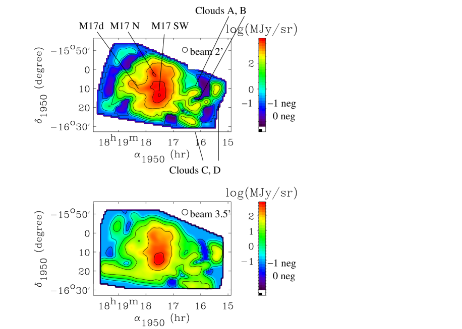
Figure 1: PRONAOS intensity maps in band 1 (200 ${\mu}m$, up) and band 4 (580 ${\mu}m$, bottom). The angular resolution is 2^′ for the 200 ${\mu}m$ map and 3.5^′ for the 580 ${\mu}m$ map. The color scale is logarithmic, and displays the positive reconstructed intensity until -1 in log, then the deeper blue and purple colors display the negative noise features. The noise level is about 4 MJy/sr rms in band 1 and 0.8 MJy/sr in band 4. Due to the calibration uncertainty, the intensity accuracy is 5 % (1 $\sigma$) relative between bands (8 % absolute). The non-observed areas are displayed in white.

Table 1: Equatorial coordinates and fluxes (Jy) integrated over a 3.5^′ area, around the intensity peaks of the identified regions. The absolute errors on the fluxes are 8 % (1 $\sigma$). These values take into account the fine color corrections due to the large bandwidths of the SPM instrument.

	$\alpha_{1950}$	$\delta_{1950}$	Fν(Jy)	Fν(Jy)	Fν(Jy)	Fν(Jy)
	(h,min,sec)	(o,′)	200 ${\mu}m$	260 ${\mu}m$	360 ${\mu}m$	580 ${\mu}m$
M17 SW	18 17 35	-16 15	28000	15000	6600	1500
M17 N	18 17 45	-16 03	4800	2500	1200	290
Cloud A	18 16 22	-16 12	340	210	120	25
Cloud B	18 16 16	-16 20	280	210	130	36
Cloud C	18 16 29	-16 28	260	160	98	31
Cloud D	18 15 34	-16 11	240	210	140	44

The maps in Fig. 1 exhibit the very high intensity contrasts that exist in this kind of giant molecular complex. The M17 Southwest (SW) and North (N) areas show up as the most intense dust emission on our maps. The M17 SW cloud reaches a peak intensity of 46000 MJy/sr in band 1 (200 ${\mu}m$ with a 2^′ angular resolution) at the M17a source (see Lada (1976), Wilson et al. (1979) and Gatley et al. (1979)). A small intense condensation is visible to the northeast of the most intense area. It shows up clearly in Fig. 1 with the second highest contour in the 200 ${\mu}m$ image, and has a peak intensity of 9600 MJy/sr at 200 ${\mu}m$. This condensation corresponds to the M17b source. The M17 North condensation (also called M17c) reaches a peak intensity of 7800 MJy/sr at 200 ${\mu}m$. The M17d source (Wilson et al. (1979)) is clearly visible to the east from M17b, and reaches a 200 ${\mu}m$ peak intensity of 2000 MJy/sr .

We have also mapped the area to the west of the M17 complex, in which we can identify four condensations with weak intensities. Cloud A (see Fig. 1 for the names) is situated west of M17 SW and shows up as an extended condensation reaching a 200 ${\mu}m$ peak intensity of 630 MJy/sr . Cloud B is south of Cloud A and is linked to it by a bridge clearly visible on the maps. Cloud B reaches a 200 ${\mu}m$ peak intensity of 440 MJy/sr . Another extended condensation, that we call Cloud C, is visible south of Cloud B. It has a peak intensity of 470 MJy/sr . Cloud D is a condensation situated to the northwest of the maps, linked to Cloud B through a filament, inside which a small (2^′) condensation is visible. Cloud D has a 200 ${\mu}m$ peak intensity of 470 MJy/sr .

It is worth mentioning that these weak-intensity clouds are poorly visible in the IRAS 100 ${\mu}m$ survey. As we can see in Fig. 1, the PRONAOS 580 ${\mu}m$ map looks smoother than the 200 ${\mu}m$ one, exhibiting less intensity contrast between regions. As we shall discuss later, this is due to a trend of the intense areas to have warmer dust than the faint ones. This induces a stronger relative intensity of the weak-intensity areas in long-wavelength bands, therefore reducing the contrast between the regions in the long-wavelength maps.

4 Analysis

4.1 Dust temperatures and spectral indices

4.1.1 Derivation

We assume that the emission of the grains is characterized by the modified blackbody law:

$$I_{\nu fit}(\lambda,T,\beta)=C\;{B_{\nu}}(\lambda,T)\;\lambda^{-\beta}$$ (1)

where $\lambda$ is the wavelength, C a constant, T the temperature of the grains, $\beta$ the spectral index and ${B_{\nu}}$ the Planck function. The fit procedure is described in detail in Dupac et al. (2001). In this work, we included iteratively the color correction process due to the SPM bandwidths. Assuming optically thin emission, we can derive the optical depth $\tau_{\nu}={I_{\nu}\over{B_{\nu}}}=C\;\lambda^{-\beta}$. The relative error on $\tau_{\nu}$ is ${\Delta I_{\nu}\over I_{\nu}}+{h\nu\over kT^{2}}\Delta T$.

We show the temperature and spectral index maps derived this way in Fig. 3. These have been made without assuming anything about the temperature or the spectral index. We used the IRAS 100 ${\mu}m$ data for the determination of the temperature and the spectral index of a large part of the map (for this we assumed an intercalibration error between IRAS and PRONAOS data of 25 %), but neither for M17 SW (saturated) nor for the faint clouds A, B, C, D to the west, for which the IRAS 100 ${\mu}m$ data seem too noisy. In the areas where the fit was difficult because of the high temperatures estimated ($>$ 70 K), we used the IRAS 60 ${\mu}m$ data too. This is justified by considering that the thermal continuum of big grains dominates the 60 ${\mu}m$ emission for such high temperatures, whereas it is likely not to be the case for lower temperatures for which the very small grains might dominate the 60 ${\mu}m$ emission. With this process, the fit is performed in each pixel where the signal to noise ratio is reasonable. However, some observed areas are too noisy to obtain an estimation of the temperature and the spectral index. These areas are displayed in white on the maps in Fig. 3. We present spectra of some observed M17 regions in Fig. 2.

Figure 2: Spectra with 3 $\sigma$ error bars. The PRONAOS error bars are the intercalibration errors. The 100 ${\mu}m$ point is from the IRAS survey. The drawn lines are the result of the fits (modified black body).

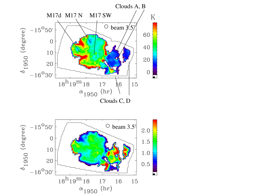
Figure 3: Maps of the dust temperature in Kelvin (top) and the spectral index (bottom), made by fitting the modified blackbody to the PRONAOS spectra, with the IRAS 100 ${\mu}m$ and 60 ${\mu}m$ data for some regions. The angular resolution is 3.5^′ in each map. The external contour shows the limit of the observed area. The white regions inside this contour are too noisy to obtain an estimation of the temperature and the spectral index.

Table 2: Temperature, spectral index and optical depth of the intensity peaks of the identified regions. The error bars are given for the 68 % confidence interval.

	T (K)	$\beta$	$\tau_{\nu}\centerdot 10^{3}$	$\tau_{\nu}\centerdot 10^{3}$
			200 ${\mu}m$	580 ${\mu}m$
M17 SW	29 $\pm$ 8	1.7 $\pm$ 0.3	80 $\pm$ 60	12 $\pm$ 3
M17 N	28 $\pm$ 3	1.6 $\pm$ 0.2	15 $\pm$ 6	2.6 $\pm$ 0.4
Cloud A	17 $\pm$ 3	2.3 $\pm$ 0.3	6 $\pm$ 4	0.5 $\pm$ 0.1
Cloud B	17 $\pm$ 3	1.7 $\pm$ 0.3	5 $\pm$ 3	0.7 $\pm$ 0.2
Cloud C	26 $\pm$ 4	1.2 $\pm$ 0.2	1 $\pm$ 0.5	0.3 $\pm$ 0.07
Cloud D	14 $\pm$ 2	1.9 $\pm$ 0.3	9 $\pm$ 6	1.3 $\pm$ 0.3

4.1.2 Variations of the temperature and the spectral index

The maps in Fig. 3 exhibit interesting features: first, it is evident comparing the maps that an anticorrelation exists between the temperature and the spectral index. We shall quantify this later. In the major part of the maps, the temperature ranges from 10 K to 80 K, while the spectral index exhibits also large spatial variations from 1 to more than 2.5. Temperatures above 80 K (around 100 K or higher) can be found in a few pixels near the ionization front to the east. Large scale features on these maps are clearly visible, showing how the temperature increases from the west to the east. The weak intensity areas to the west are significantly colder than the intense M17 area. We present in Table LABEL:resul the temperature, spectral index and optical depth for the intensity peaks of the identified regions (Fig. 1). The M17 SW region shows a temperature of 29 K ($\pm$ 8) at the intensity peak. For this area, we derive a spectral index of 1.7 ($\pm$ 0.3). However, since the IRAS data are saturated in this area, the fit is quite uncertain and the temperature could be higher. The M17 N condensation has a temperature of 28 K, and a spectral index of 1.6. The temperature in the M17 complex is about 30-50 K outside the M17 SW and M17 N condensations, and the spectral index varies between 1 and 1.5. On the edges of the complex, one can see the warm areas near the ionized regions (east and north-west), where the temperature can be higher than 80 K, and the spectral index between 0.7 and 1.1. The clouds A, B, and D in the western part of the maps show low temperatures (14-17 K) and high spectral indices (1.7-2.3). Some areas in these clouds even exhibit very low temperatures down to 10 K.

4.1.3 Anticorrelation between the temperature and the spectral index

As we can see in Fig. 3, it seems that an anticorrelation exists between the temperature and the spectral index. This effect was shown for the first time in observations by Dupac et al. (2001) in Orion. If we take the five intensity peaks presented in Table LABEL:resul, the correlation coefficient is -0.58, which means a significant anticorrelation. However, it is not highly statistically significant, given the small number of points. Therefore, we have analyzed the correlation between the temperature and the spectral index in the whole map. We present in Fig. 4 a plot of the distribution of the pixels in Fig. 3 in the (T,$\beta$) space.

Figure 4: Distribution in the (T,$\beta$) space of the (T,$\beta$) pairs derived with both errors on T and $\beta$ lower than 20 %.

One can see the banana shape of this distribution in Fig. 4, which clearly shows the anticorrelation between both parameters. In particular, very few pixels can be found in the data with T $>$ 40 K and $\beta$ $>$ 1.5, and no pixel can be found with T $<$ 20 K and $\beta$ $<$ 1.6. If we consider all the (T,$\beta$) pairs with T between 10 K and 80 K, and $\beta$ between 1 and 2.5, then the correlation coefficient is -0.56. Among these 1079 pixels, 1071 have both temperature and spectral index with relative errors less than 50 %, and 801 with relative errors less than 20 %. The correlation coefficient computed from these 801 well fitted pixels is -0.64. If we consider only the pixels with relative errors less than 10 % (87 pixels), then the correlation is -0.74. This increasing of the anticorrelation with the restriction on the errors is evidence of the reality of this effect. Also, pixels with high spectral indices have narrow error bars on the spectral index: there are 70 pixels for 2.3 $<\beta<$ 3, with an average relative error on $\beta$ of 12 % - the relative errors are quite uniform for these points. Pixels with low spectral indices also show quite narrow error bars: there are 482 pixels for 0.7 $<\beta<$ 1.3, with an average relative error on $\beta$ of 16 %. Therefore, we can be confident of this anticorrelation effect. Nevertheless, to better understand it, we performed simulations of PRONAOS data from the same number (801) of random (T,$\beta$) pairs in the same (T,$\beta$) range, and fitted them the same way as real data. We repeated this processing with several distributions of T-$\beta$ pairs without intrinsic correlation, with and without 100 ${\mu}m$ simulated data, and obtained correlation coefficients on the fitted parameters usually between 0.0 and -0.2, and never above (in absolute) -0.3. Therefore, the fit procedure itself involves some degree of anticorrelation between the derived temperature and spectral index, as Dupac et al. (2001) had already investigated. There is indeed some degeneracy between both parameters, but this correlation coefficient which we find on simulations is clearly not enough to explain the correlation found on the data (-0.64). Thus we have to conclude that this anticorrelation effect has to be either an intrinsic physical property of the grains, or at least a property of the observed dust, when integrated on the beam and the ISM column. The same effect has been shown in Orion (Dupac et al. (2001)).

To interpret this anticorrelation, we can investigate what the meaning is of such spectral index variations. Mixtures of dust components with different temperatures can be put forward: this clearly cannot explain high indices, but could explain low indices around 1. Indeed, warm dust can be associated in the same line of sight with cold dust components which could enhance the high-wavelength intensity, and therefore decrease the spectral index from 2 to around 1. However, this would imply a large amount of cold dust (see the investigations of Ristorcelli et al. (1998) and Dupac et al. (2001)). In this article, we have performed other studies. We simulate spectra with low spectral indices and various warm temperatures. We then try to fit these spectra with two dust components having both a “standard” spectral index equal to 2, the warm component having the same 100 ${\mu}m$ emission and the same temperature as the single component spectrum. Thus we have equality between both optical depths ($C\;\lambda^{-\beta}$) at 100 ${\mu}m$, and therefore, given the simple column density model that we present in Section 4.2, the warm dust component has the same column density as the single dust component. In this way, we fit the short-wavelengths part of the original spectrum by the warm component, but the discrepancy between the original spectral index and the standard one ($\beta$ = 2) induces a lack of emissivity of the warm component compared to the original spectrum at long wavelengths. Therefore, we introduce a colder dust component with the same standard spectral index $\beta$=2, which we add to the warm component to fit the spectrum. Then we can investigate what amount of cold dust is necessary to explain the observed low spectral indices, by computing the column densities from our simple model (see Section 4.2 and Dupac et al. 2001). Indeed, with two dust components with the same standard spectral index, the column density ratio between both is simply the ratio of the parameters C.

Table 3: Summary of the investigations made concerning the two-dust component assumption. From left to right: the original spectrum temperature, the original spectral index, the temperature of the cold component, which has a spectral index $\beta$=2, and the mass ratio derived between the cold and warm components.

T (K)	$\beta$	Tcold (K)	Mass ratio
50	1	10	100
70	1	10	200
60	1	20	20
60	1	40	no fit
50	1.5	10	50
50	1.5	20	5
50	1.5	30	3, bad fit
40	1.7	10	20

We present in Table LABEL:twocomp a summary of these investigations. It appears that low indices (around 1) would imply very large amounts of cold dust in the line of sight. For example, to fit this way a spectrum with T = 50 K, $\beta$ = 1, with a 10 K component, a cold dust column density 100 times larger than the warm dust column density is necessary. We have said that the column density of the warm component is the same as the single dust-method one. As seen in Table LABEL:masses, the column density estimates, assuming one dust component, seem to have the right order of magnitude, compared for example to the estimates from the CO. It is extremely unlikely that there are such huge amounts of cold dust (much larger than the warm dust and the CO estimates) in each line of sight where we observe low indices. If one uses intermediate temperatures for the cold component, then it is no longer possible to match the spectrum at long wavelengths, even for $\beta$=1.5. We show by these investigations that even for intermediate spectral indices, it is unlikely that they be explained only by temperature mixtures with the same standard spectral index.

Moreover, the shape of the pixel distribution in the (T, $\beta$) space is very difficult to explain with only the argument of temperature mixtures. It would suggest that the warmer the (warm) dust component, the more massive the cold component, because the spectral index is further reduced (to 1) at high temperatures. This can certainly not be a general rule, and this shows that the temperature mixture assumption is insufficient to explain the variations found on the spectral index and its inverse dependence on the temperature.

Laboratory experiments (see Agladze et al. (1996) and Mennella et al. (1998)) showed this anticorrelation effect on grains for temperatures down to 10 K. Agladze et al. (1996) measured absorption spectra of crystalline and amorphous grains between 0.7 and 2.9 mm wavelength. They deduced an anticorrelation between the power-law index $\beta$ and the temperature in the temperature range 10-25 K, and attributed it to two-level tunnelling processes. The measures of Agladze et al. (1996) are insufficient to justify our observation in the submillimeter spectral range, because absorption can be very different in the millimeter range. Mennella et al. (1998) measured the absorption coefficient of cosmic dust grain analogues, crystalline and amorphous, between 20 ${\mu}m$ and 2 mm wavelength, in the temperature range 24-295 K. They deduced an anticorrelation between T and $\beta$, and attributed it to two-phonon difference processes. In our observations, we observe this effect down to about 10 K (Fig. 4), thus we would need laboratory results on these low temperatures in the submillimeter range to fully understand the observations. Other causes can make the spectral index vary, such as the composition and size of the grains.

We can conclude from this temperature-spectral index analysis that the anticorrelation discovered by Dupac et al. (2001) in Orion is shown in M17 too, another high-mass star-forming complex of our Galaxy. Our investigations make us rather believe in a fundamental property of the grains to explain this effect.

4.2 Column densities

We are interested in estimating the column densities and masses of the studied region. For this we follow the simple model described in Dupac et al. (2001), which uses the dust 100 ${\mu}m$ opacity from Désert et al. (1990). We derive column densities that we present in Table LABEL:masses. To obtain an independent estimation of the column density, we use observations of the rotational transition $J=1-0$ of ${}^{13}CO$, made by Wilson et al. (1999). Their map covers the M17 cloud but not the fainter area to the west. Assuming local thermal equilibrium and optically thin emission, the ${}^{13}CO$ column density can be expressed as:

$$N_{{}^{13}CO}=2.6\>10^{14}\;{W_{{}^{13}CO}\over(1-e^{-5.3/T})}$$ (2)

(see e.g. Rohlfs et al. (2000)) Then, assuming a ${H_{2}\over{}^{13}CO}$ number ratio of 4.6 $10^{5}$ (Rohlfs et al. (2000)), a mean molecular weight of 2.36 $m_{H}$ (see e.g. Elmegreen et al. (1979)), and a temperature of the gas of 30 K, we derive a column density to ${}^{13}CO$ line ratio of 17 $10^{20}$ protons $cm^{-2}(K.km/s)^{-1}$. Using this coefficient, we derive column densities that we present in Table LABEL:masses, in order to compare to the PRONAOS + Désert model estimation.

Table 4: Column densities estimated from the PRONAOS+Désert method, and from the ¹³CO data of Wilson et al. (1999), masses from PRONAOS+Désert, PRONAOS+Ossenkopf, Jeans masses. The error bars on the PRONAOS+Désert column densities are given for the 68 % confidence interval.

	NH PRONAOS+Dés.	NH 13CO	Mass PRONAOS+Dés.	Mass PRONAOS+Oss.	Jeans mass
	$10^{20}Hcm^{-2}$	$10^{20}Hcm^{-2}$	M⊙	M⊙	M⊙
M17 SW	4100 $\pm 3600$	1200	16000	—	—
M17 N	730 $\pm 340$	460	4600	—	—
Cloud A	450 $\pm 380$	—	2000	730	70
Cloud B	250 $\pm 210$	—	2400	870	100
Cloud C	38 $\pm 25$	—	350	—	150
Cloud D	630 $\pm 530$	—	2100	760	100

The agreement is not very good in M17 SW between PRONAOS + Désert model and ¹³CO, though it is consistent with the error bar. It is not unlikely that this is due to optical thickness of the ¹³CO 1-0 emission. The M17 N region shows a better agreement. If we trust our PRONAOS + Désert model estimation (which seems quite speculative in view of the error bars), we can constrain the column density to ${}^{13}CO$ line ratio in M17, which we find to range roughly from 15 $10^{20}$ to 100 $10^{20}$ following the regions of M17 (in units of protons $cm^{-2}(K.km/s)^{-1}$). Since the ratio corresponding to optically thin ${}^{13}CO$ emission is 17 $10^{20}$, and that the most intense areas have the highest coefficient, it is possible to conclude that the disagreement between PRONAOS and ${}^{13}CO$ column density estimations of M17 SW may be due (at least in a part) to optical thickness of the ${}^{13}CO$ 1-0 line. Also, uncertainties in the ${H_{2}\over{}^{13}CO}$ ratio may arise for high column densities. Moreover, the excitation temperature can be higher than 30 K in M17 SW, although we measure it to be around 30 K. If we take an excitation temperature of 60 K, then the column density estimated from the ${}^{13}CO$ emission is 2300 $10^{20}$ H $cm^{-2}$ for M17 SW (at the intensity peak). If now we look at the sources of uncertainties in the PRONAOS + Désert model estimation - apart from the error bars being large, we can point out that the 100 ${\mu}m$ opacity we used might overestimate the column density, especially in cold clouds where could take place some special effects like formation of molecular ice mantles on the grains and coagulation of grains. For instance, these processes are taken into account by the protostellar core model of Ossenkopf & Henning (1994), for which the 100 ${\mu}m$ opacity is 1 $cm^{2}/g$. By making the same analysis as with the model of Désert et al. (1990), using the Ossenkopf & Henning opacity, we derive column densities 2.8 times lower. This correction could be true for cold clouds like A, B and D.

Finally, we computed masses of regions in this giant molecular complex. For this, we integrated the column density found from our submillimeter measurement over the area of the clouds that we observe in the maps, assuming a distance of 2200 pc (Chini et al. (1980)). By this way, we derive a total ISM mass of the M17 complex (without Clouds A, B, C, D to the west) of 31000 M_⊙, in which M17 SW weights 16000 M_⊙ and M17 N 4600 M_⊙. We derive also mass estimates of the clouds to the west, which we present in Table LABEL:masses. For the cold clouds A, B and D, it is likely that the masses are smaller than that: if we trust the Ossenkopf & Henning (1994) model, then we derive masses of about 800 M_⊙ for each. For the clouds separated from the molecular complex (A, B, C, D), we present also in Table LABEL:masses the Jeans masses, as an indicator of the gravitational stability of these condensations (see Dupac et al. (2001) for details). There are of course large uncertainties in both the clump’s measured mass and the non-thermal sources of internal energy, such as magnetic field and turbulence, which can help to balance the gravitational energy. Nevertheless, we observe that Clouds A, B and D are possibly gravitationally unstable, especially Cloud A, which might be compressed by the external pressure due to the ionized area to the north.

5 Conclusion

We observed a large (50^′ x 30^′, $\approx$ 30 pc x 20 pc) area in and around the M17 molecular complex. We showed extended faint clumps (A, B, C, D) in the outskirts of the active star-forming area. Our study shows a large distribution of temperatures and spectral indices: the temperature varies roughly from 10 K to 100 K, and the spectral index from 1 to 2.5. The statistical analysis of the temperature and spectral index spatial distribution shows the anticorrelation between these two parameters. Indeed, we observe cold dust (10-20 K) with high indices (around 2), and warm dust ($>$ 20 K) with low indices (around 1 - 1.5), but we could not significantly find any cold place with low indices nor warm place with high indices. The investigations which we made to match the observed spectra, with two dust components having a standard spectral index, imply very large and unlikely amounts of cold dust, therefore we rather support a fundamental explanation for this effect. Laboratory measurements showed this anticorrelation in the submillimeter domain on grains for temperatures down to 25 K, but we would need laboratory results on temperatures down to 10 K in the submillimeter range to fully understand our observations. This anticorrelation effect was also shown in Orion (Dupac et al. (2001)), and in other PRONAOS observations that are still being analyzed.

We estimated the column densities and masses of the observed regions by simply modelling the thermal emission of the grains from Désert et al. (1990) or Ossenkopf & Henning (1994). We derived a total mass of the M17 cloud of 31000 M_⊙. Of course, the error bars are large and difficult to estimate properly, but there is a clear trend for three cold clouds (A, B, D) to be gravitationally unstable, and therefore to be pre-stellar candidates.

These observations could be sustained by sensitive continuum observations in the millimeter domain, especially for the faint clouds studied to the west of the M17 complex, in order to better constrain the spectral index measurement of the cold dust. Also, infrared observations at higher resolution could be useful to study the structure of these cold clouds.

6 Acknowledgements

We thank very much Christine Wilson and her collaborators for having provided us their ${}^{13}CO$ data. We are indebted to the French space agency Centre National d’Études Spatiales (CNES), which supported the PRONAOS project. We are very grateful to the PRONAOS technical teams at CNRS and CNES, and to the NASA-NSBF balloon-launching facilities group of Fort Sumner (New Mexico).

References

- Agladze et al. (1996) Agladze, N.I., Sievers, A.J., Jones, S.A., Burlitch, J.M., Beckwith, S.V.W.: 1996, ApJ, 462, 1026
- Buisson & Duran (1990) Buisson, F., Duran, M.: 1990, Proc. 29th Liège Colloq., ed. B. Kaldeich (Paris: ESA), 314
- Chini et al. (1980) Chini, R., Elsässer, H., Neckel, T.: 1980, A&A, 91, 186
- Désert et al. (1990) Désert, F.-X., Boulanger, F., Puget, J.L.: 1990, A&A, 237, 215
- Dupac et al. (2001) Dupac, X., Giard, M., Bernard, J.-P., Lamarre, J.-M., Mény, C., Pajot, F., Ristorcelli, I., Serra, G., Torre, J.-P.: 2001, ApJ, 553, 604
- Dupac & Giard (2002) Dupac, X., Giard, M.: 2002, MNRAS, 330, 497
- Elmegreen et al. (1979) Elmegreen, B.G., Lada, C.J., Dickinson, D.F.: 1979, ApJ, 230, 415
- Emerson et al. (1979) Emerson, D.T., Klein, U., Haslam, C.G.T.: 1979, A&A, 76, 92
- Gatley et al. (1979) Gatley, I., Becklin, E.E., Sellgren, K., Werner, M.W.: 1979, ApJ, 233, 575
- Glushkov (1998) Glushkov, Y.I.: 1998, Astronomy Reports, 42, 137
- Harper et al. (1976) Harper, D.A., Low, F.J., Rieke, G.H., Thronson, H.A.: 1976, ApJ, 205, 136
- Harper & Low (1971) Harper, D.A., Low, F.J.: 1971, ApJ Lett., 165, L9
- Lada (1976) Lada, C.J.: 1976, ApJ Suppl., 32, 603
- Lamarre et al. (1994) Lamarre, J.-M., et al. : 1994, Infrared Phys. Tech., 35, 277
- Low & Aumann (1970) Low, F.J., Aumann, H.H.: 1970, ApJ Lett., 162, L79
- Mennella et al. (1998) Mennella, V., Brucato, J.R., Colangeli, L., Palumbo, P., Rotundi, A., Bussoletti, E.: 1998, ApJ, 496, 1058
- Ossenkopf & Henning (1994) Ossenkopf, V., Henning, T.: 1994, A&A, 291, 943
- Rainey et al. (1987) Rainey, R., White, G.J., Gatley, I., Hayashi, S.S., Kaifu, N., Griffin, M.J., Monteiro, T.S., Cronin, N.J., Scivetti, A.: 1987, A&A, 171, 252
- Ristorcelli et al. (1998) Ristorcelli, I., Serra, G., Lamarre, J.M., Giard, M., Pajot, F., Bernard, J.P., Torre, J.P., De Luca, A., Puget, J.L.: 1998, ApJ, 496, 267
- Rohlfs et al. (2000) Rohlfs, K., Wilson, T.L., Hüttemeister, S.: 2000, Tools of Radioastronomy, Springer A&A Library
- Sales et al. (1991) Sales, N., Chabaud, J.-P., Giard, M., Brockman, B., Clavier, J.-P.: 1991, Experimental Astron., 2, 1
- Sekimoto et al. (1999) Sekimoto, Y., et al. : 1999, proc. of Star Formation 1999, Nagoya, Ed.: T. Nakamoto
- Serra et al. (2001) Serra, G., Giard, M., Bernard, J.-P., Stepnik, B., Ristorcelli, I.: 2001, C.R. Acad. Sci. Ser. IV, 1, 1215-1222
- Wilson et al. (1979) Wilson, T.L., Fazio, G.G., Jaffe, D., Kleinmann, D., Wright, E.L., Low, F.J.: 1979, A&A, 76, 86
- Wilson et al. (1999) Wilson, C., Howe, J., Balogh, M.: 1999, ApJ, 517, 174