On Validating an Astrophysical Simulation Code

Abstract

We present a case study of validating an astrophysical simulation code. Our study focuses on validating FLASH, a parallel, adaptive-mesh hydrodynamics code for studying the compressible, reactive flows found in many astrophysical environments. We describe the astrophysics problems of interest and the challenges associated with simulating these problems. We describe methodology and discuss solutions to difficulties encountered in verification and validation. We describe verification tests regularly administered to the code, present the results of new verification tests, and outline a method for testing general equations of state. We present the results of two validation tests in which we compared simulations to experimental data. The first is of a laser-driven shock propagating through a multi-layer target, a configuration subject to both Rayleigh-Taylor and Richtmyer-Meshkov instabilities. The second test is a classic Rayleigh-Taylor instability, where a heavy fluid is supported against the force of gravity by a light fluid. Our simulations of the multi-layer target experiments showed good agreement with the experimental results, but our simulations of the Rayleigh-Taylor instability did not agree well with the experimental results. We discuss our findings and present results of additional simulations undertaken to further investigate the Rayleigh-Taylor instability.

1 Introduction

The enormous progress seen in the evolution of fast computing machines and numerical methods stands as one of the great achievements of the twentieth century. Numerical modeling is now an accepted and widely applied method of research, and in many cases simulations have matured to the extent that they now provide direction to theoretical research. In astrophysics, where the complexity of many of the problems requires large-scale computing for any hope of progress, much of research involves the development and application of reliable and trustworthy simulation codes. Before the scientific community can have confidence in results from such a code, it must be subjected to a wide variety of verification and validation tests. This paper discusses progress in verification and validation of FLASH, a parallel, adaptive-mesh simulation code for the compressible, reactive flows found in many astrophysical environments.

The goal motivating the development of FLASH is to advance the solution of several astrophysical problems related to thermonuclear flashes on the surfaces and in the interiors of compact objects. In particular, the problems of interest are type I X-ray bursts, classical novae, and Type Ia supernovae. These events all involve the accretion of material from a companion star onto the surface of the compact star, followed by the ignition of either the core of the compact star or the material accreted onto the surface. The global physical phenomena common to all three of these events include an accretion flow onto the surfaces of compact stars, shear flow and Rayleigh-Taylor instabilities (Taylor, 1950; Chandrasekhar, 1981) on the stellar surfaces and in the core, ignition of thermonuclear burning in degenerate matter, development of convection, propagation of nuclear burning fronts, and expansion of the stellar envelope. An understanding of these global phenomena requires knowledge of the fundamental physical processes involved in each. Accordingly, much of our scientific effort focuses on research into the basic “microphysics.” These fundamental processes include turbulence at large Reynolds and Rayleigh numbers, fluid instabilities and mixing, convection and the convective penetration of stable matter at very high densities, thermodynamics in relativistic and degenerate regimes, the propagation of both subsonic and supersonic burning fronts, and radiation hydrodynamics.

Verification and validation are fundamental steps in developing any new technology, whether it be a simulation code like FLASH or an instrument for observation. For simulation technology, the goal of these testing steps is assessing the credibility of modeling and simulation. Considerable work on verification and validation of simulations has been done in the field of computational fluid dynamics (CFD), and in the CFD literature the terms verification and validation have precise, technical meanings (AIAA, 1998; Roache, 1998a, b). Verification is taken to mean demonstrating that a code or simulation accurately represents the conceptual model. Validation of a simulation means demonstrating that the simulation appropriately describes nature. The scope of validation is therefore much larger than that of verification and includes comparison of numerical results with experimental or observational data. In astrophysics, where it is difficult to obtain observations suitable for comparison to numerical simulations, this process can present unique challenges.

In this paper, we describe our efforts at verifying and validating the hydrodynamics module in FLASH. We begin by describing the astrophysical problems of interest and the importance of fluid instabilities in the problems. A discussion of the terminology and methodology for verification and validation (V&V) follows this description. We follow that with a discussion of the challenges found in verifying and validating astrophysical simulations, and in particular, the aspects of astrophysical modeling for which it is difficult to apply recommended CFD V&V techniques. In the next section, we present verification tests and include an outline of a procedure for testing an arbitrary equation of state in the context of numerical hydrodynamics schemes. The following section contains a comparison of the results from two laboratory experiments with those obtained from simulations, and the final section contains discussion and conclusions.

1.1 Overview of Astrophysical Thermonuclear Flashes

Thermonuclear flashes, events of rapid or explosive thermonuclear burning, occur in a variety of stellar settings. These events include type I X-ray bursts, classical novae, and Type Ia supernovae, all of which involve a close binary system in which matter from a companion star accretes onto the surface of a compact star (neutron star or white dwarf). Either the core of the compact object or the accreted layer on the surface of the compact object ignites under electron-degenerate conditions, and a thermonuclear burning front is born and begins to propagate.

These events provide not only fantastic observational displays, but also tools with which potentially to answer several fundamental questions. The light curves and spectra of X-ray bursts can provide information about the masses and radii of neutron stars (Lewin, van Paradijs, & Taam, 1993; Lamb, 2000) and thus also provide information about the nuclear equation of state. Classical novae can provide information about the abundances of intermediate-mass elements in the universe and the dynamics of white dwarfs in close binary systems (Gehrz et al., 1998). Type Ia supernovae provide additional information about the abundances of intermediate-mass and heavy elements and play a crucial role as “standard candles” in determining cosmological parameters such as the Hubble constant, $H_{0}$, the mass density, $\Omega_{M}$, and the cosmological constant or vacuum energy density, $\Omega_{\Lambda}$ (see Riess et al., 1998; Perlmutter et al., 1998; Turner, 2001, and references therein).

X-ray bursts are flashes that start at the bottom of a very thin layer ($\sim 10-100$ m) of hydrogen-rich or helium-rich fuel that has accreted onto the surface of a neutron star (Taam, 1985; Lewin, van Paradijs, & Taam, 1993; Taam et al., 1993). The total energy released by burning the fuel into ash is a factor of $\sim 20-100$ less than the gravitational binding energy. Consequently, the accreted material is gravitationally bound to the neutron star and the flash is not quenched by expansion of the envelope (Hansen & Van Horn, 1975). Instead, fuel in the accreted envelope is incinerated to iron-peak or heavier nuclei (Shatz et al., 2001).

Novae result from the ignition of a layer ($\sim 10^{4}$ m) of hydrogen-rich material that has accreted onto the surface of a white dwarf (Truran, 1982; Shara, 1989; Starrfield, 1989; Livio, 1994). In this case, the total energy released by thermonuclear burning is a factor of $\sim$ 100 more than the gravitational binding energy. As a result, the excess energy leads to an enormous expansion of the white dwarf’s envelope, which engulfs the companion star and forms a common envelope binary. The work done against gravity in the expansion of the envelope cools the hydrogen burning layer and quenches the runaway, leading to the establishment of a phase of stable hydrogen burning that continues through envelope exhaustion.

Type Ia supernovae are thought to be due to carbon flashes that ignite in the cores of accreting white dwarfs (Woosley & Weaver, 1986; Nomoto, Yamaoka, & Shiegeyama, 1994; Niemeyer, 1995; Niemeyer & Hillebrandt, 1995). Models involving either a pure deflagration or a pure detonation have been unable to provide a consistent explanation for the observed expansion velocities and the spectrum of intermediate-mass and iron-peak ejecta. Some Type Ia supernova models that involve a transition from a deflagration to a detonation have been constructed. One possibility is a more-or-less spontaneous transformation of the initial deflagration into a detonation as the burning front propagates outward through the white dwarf (Niemeyer, 1995; Niemeyer & Hillebrandt, 1995; Khokhlov, Oran, & Wheeler, 1997; Niemeyer & Woosley, 1997). Another possibility is that the initial deflagration dies out as a result of the expansion of the outer layers of the white dwarf. When these gravitationally bound layers collapse back onto the white dwarf, a detonation is ignited (Blinnikov & Khokhlov, 1987; Boisseau et al., 1996; Khokhlov, 1995; Khokhlov, Oran, & Wheeler, 1997). In either case, these models are capable of accounting for the observed expansion velocities of the silicon-group and iron-group nuclei.

In all three of these thermonuclear flash events, the nuclear burning time scale is much shorter than the time scale over which the nuclear fuel accretes onto the surface. These short burning time scales make it likely that ignition of the fuel occurs at either a single point or, at most, at a few discrete points. The situation may be complicated by the presence of magnetic fields. The strong magnetic fields (B $\sim 10^{6}$ - $10^{9}$ G) of white dwarfs and the super-strong magnetic fields (B $\sim 10^{9}$ - $10^{12}$ G) of neutron stars may be capable of funneling the flow of accreting matter onto the magnetic polar caps of the compact object (Lamb, Pethick, & Pines, 1973). The accreted matter, which constitutes the nuclear fuel, may or may not be able to spread over the surface of the star before ignition occurs. The three-dimensional nature of this fuel geometry is compounded by the effects of a magnetic field on the thermal and mass transport coefficients (Lamb, Miller, & Taam, 1996; Potekhin, 1999; Potekhin, et al., 1999).

Even in the absence of a magnetic field, thermonuclear flashes are inherently multi-dimensional because of the complexity of the underlying fluid instabilities. Most efforts at modeling the multi-dimensional nature of thermonuclear flashes have been two-dimensional (Fryxell & Woosley, 1982; Steinmetz, Müller & Hillebrandt, 1992; Shankar, Arnett, & Fryxell, 1992; Shankar & Arnett, 1994; Livne, 1993; Glasner & Livne, 1995; Glasner, Livne, & Truran, 1997; Khokhlov, 1995; Boisseau et al., 1996; Kercek, Hillebrandt & Truran, 1998), but there have been a few three-dimensional studies (Khokhlov, 1995; Khokhlov, Oran, & Wheeler, 1997; García-Senz, Bravo, & Woosley, 1999; Kercek, Hillebrandt, & Truran, 1999). Recent progress includes a detailed two-dimensional study of helium detonations on the surface of a neutron star that confirmed that a detonation can spread burning over the entire surface on a time scale consistent with burst rise times (Zingale et al., 2001), three-dimensional simulations of thermonuclear explosions of Chandrasekhar-mass carbon-oxygen white dwarfs (Reinecke, Hillebrand, & Niemeyer, 1999), and studies of the cellular structure of detonation fronts in both two and three dimensions (Timmes et al., 2000, 2002).

1.2 The Role of Fluid Instabilities in Flash Problems

Fluid instabilities and subsequent mixing are expected to play a fundamental role in the events involving thermonuclear flashes. For example, determining whether or not there is substantial mixing between the accreted hydrogen-helium envelope and the carbon-oxygen surface layer of the white dwarf is crucial to understanding the nova mechanism. Mixing of intermediate-mass elements into the accreted layer is critical because otherwise hydrogen burning would be too slow to produce a nova. Furthermore, without this mixing it is difficult to produce the observed abundances of intermediate-mass nuclei in the ejecta (see Rosner et al., 2001, and references therein). Such mixing may occur during the first phases of the accretion cycle or when convection in the accreted layer works its way down to the interface with the white dwarf. In the latter case, convective undershoot may dredge up material from the white dwarf and mix it into the accreted layer (Livio & Truran, 1990). Although some progress has been made on modeling this nova mixing mechanism (Glasner, Livne, & Truran, 1997; Kercek, Hillebrandt & Truran, 1998; Kercek, Hillebrandt, & Truran, 1999), a consensus has not been reached. Another proposed mixing mechanism, which is the subject of ongoing research, is breaking of nonlinear resonant gravity waves at the carbon-oxygen surface (Rosner et al., 2000, 2001; Alexakis, Young, & Rosner, 2002; Alexakis, et al., 2002).

In the case of a neutron star, penetration into the crust by convection in the accreted layer is strongly inhibited by the large jump in atomic weight between the heavy element crust and the hydrogen-helium composition of the accreted layer. Thus, no significant mixing by this sort of convective dredge-up is expected to occur in thermonuclear flashes involving the surface layers of a neutron star. Some mixing may occur via other mechanisms such as shear instabilities, but, unlike the nova case, the mixing of the inert heavy elements from the underlying neutron star into the accreted layer is not likely to have a significant effect on the evolution.

Fluid instabilities and mixing are also expected to play a key role in the explosion mechanism of a Type Ia supernova. A subsonic burning front that begins near the center of a massive white dwarf is subject to Kelvin-Helmholtz, Landau-Darrieus, and Rayleigh-Taylor instabilities (Khokhlov, Oran, & Wheeler, 1997; Khokhlov, 2001; Hillebrandt & Niemeyer, 2001). Growth of these instabilities dramatically increases the surface area of the burning front. This increase in surface area increases both the burning rate and the speed of the front. The dependence of the speed of the burning front on fluid instabilities is one of the reasons a study of Rayleigh-Taylor instabilities is a key component in our efforts at V&V.

Because fluid instabilities play a fundamental role in thermonuclear flash events and may be probed in reasonably good terrestrial experiments, experiments involving fluid instabilities have been the focus of our validation efforts thus far. In what follows, after describing the methodology of V&V and briefly describing our numerical methods, we present verification tests and the results of two validation problems– a laser-driven shock propagating through a multi-layer target and the classic Rayleigh-Taylor problem.

1.3 The Process of Verification and Validation

The testing step of code development, which involves verification and validation of the numerical methods and resulting simulations, is one of the most important procedures required for successful numerical modeling. This fact has been frequently overlooked in astrophysics. In our description of V&V, we take the point of view that the code to be tested is either one under development or an existing code that is being applied to a new problem. The details of testing the code will apply in either case. The results of testing will feed back to the choices of numerical methods for addressing the physics. If a particular method or model fails a test, then another must be chosen. We note that verification and validation are necessary but not sufficient tests for determining whether a code is working properly or a modeling effort is successful. These tests can only determine for certain that a code is not working properly.

V&V is a maturing area of study in the field of CFD, and there is a wealth of information available in the literature (cf. AIAA, 1998; Oberkampf, 1998; Pilch et al., 1998; Roache, 1998a, b). The fundamental strategy of V&V is the assessment of error and uncertainty in a computational simulation. The requisite methodology is complex because it must address sources of error in theory, experiment, and computation. Because these areas of study present diverse perspectives (and because V&V is still a developing field), it is common to find disagreement in the terminology of V&V (AIAA, 1998).

We adopt the following definitions from the American Institute of Aeronautics and Astronautics (AIAA) (AIAA, 1998):

• Model: A representation of a physical system or process intended to enhance our ability to understand, predict, or control its behavior.

• Modeling: The process of construction or modification of a model.

• Simulation: The exercise or use of a model. (That is, a model is used in a simulation)

• Verification: The process of determining that a model implementation accurately represents the developer’s conceptual description of the model and the solution of the model.

• Validation: The process of determining the degree to which a model is an accurate representation of the real world from the perspective of the intended uses of the model.

• Uncertainty: A potential deficiency in any phase or activity of the modeling process that is due to lack of knowledge.

• Error: A recognizable deficiency in any phase or activity of modeling that is not due to lack of knowledge.

• Prediction: Use of a CFD model to foretell the state of a physical system under conditions for which the CFD model has not been validated.

• Calibration: The process of adjusting numerical or physical modeling parameters in the computational model for the purpose of improving agreement with experimental data.

Roache (1998a) offers a concise, if informal, summary:

First and foremost, we must repeat the essential distinction between Code Verification and Validation. Following Boehm (1981) and Blottner (1990), we adopt the succinct description of “Verification” as “solving the equations right”, and “Validation” as “solving the right equations”. The code author defines precisely what partial differential equations are being solved, and convincingly demonstrates that they are solved correctly, i.e. usually with some order of accuracy, and always consistently, so that as some measure of discretization (e.g. the mesh increments) $\Delta\rightarrow 0$, the code produces a solution to the continuum equations; this is Verification. Whether or not those equations and that solution bear any relation to a physical problem of interest to the code user is the subject of Validation.

Roache goes on to point out that in a meaningful sense, a “code” cannot be validated, but only a calculation or range of calculations can be validated. He also makes the distinction between verifying a code and verifying a calculation, noting that “use of a verified code is not enough.” In our discussion, we will adhere to these definitions as closely as possible.

Another term requiring discussion is “convergence.” In CFD, the term is used in two different ways. “Grid convergence” refers to the convergence of the discretization error of the numerical solution as the grid size and time step approach zero. “Iterative convergence” refers to the convergence of the results of successive steps of an iterative procedure within a numerical method. Roache (1998a) notes that “inadequate iterative convergence will pollute grid convergence results” and that the issue of iterative convergence can blur the distinction between verifying a code and verifying a calculation because iterative tuning parameters can be problem dependent.

Figure 1, a Venn diagram (Venn, 1880) illustrating the parts of numerical modeling, provides a schematic for considering the role of verification and validation in numerical modeling. On the left, the largest circle represents Nature, or at least the part of Nature in which the problem of interest resides. The smaller circles inside of Nature represent, from largest to smallest, the range of desired validity of the code, the range of actual validity, and the range of the design goals of the code. The circle in the center of the diagram (to the right of the Nature circle) represents the theory describing Nature (which may be thought of as the model), and the circle to the right represents numerical scheme(s) implementing the theory (modeling and simulation).

Verification begins by identifying the purported design goal of the code or code modules, which is represented by the smallest circle in the center of the Nature circle on the schematic. This is the step Roache refers to as defining “precisely what partial differential equations are being solved,” though the process may require a larger scope. In the language of the AIAA, this may be thought of as identifying and understanding the implementation of the model. Verification, confirming that simulations produced by the code accurately implement the design goal of the code (i.e. the implementation accurately represents the model and the solution to the model), may be thought of as confirming the “mapping” between the theory and numerical method circles on the schematic. The process requires identification and a quantitative description of the error, and the strategy is typically a systematic study of mesh and time step refinement as is appropriate for finite difference, finite volume, and finite element methods. Other numerical methods such as vortex, lattice gas, and Monte Carlo methods require different procedures (AIAA, 1998).

Verification tests are typically simple problems, often with known analytic solutions, that can be used to study the accuracy and convergence rates of a code. Despite the relative simplicity of the tests, verification is a difficult process. Analytic solutions, which are easiest to compare against, are few and usually are limited tests of the physics. Even in these simple cases, singularities and discontinuities complicate the process of verification. Singularities arising from the geometry or the coordinate system should be removed where possible. Singularities inherent in the conceptual model (e.g. shocks and discontinuities in the flow) require special attention. These structures will typically exhibit a lower order of convergence from the rest of the flow, if indeed they lead to a converged solution at all. An added level of complexity arises in the case of discontinuous flows because not all numerical methods for solving a given set of PDEs are equivalent. Different methods handle flow discontinuities differently and/or rely on different (intrinsic numerical or physically-motivated) subgrid models. Therefore, confirming that a numerical method is correctly solving a set of PDEs can also be a validation problem.

Test problems, even without analytic solutions, may be devised to monitor conservation, symmetry properties, and effects of boundary conditions (AIAA, 1998). Additional progress may be made by testing self-convergence. Self-convergence can be difficult to test, however, and changing the resolution by a only factor of two does not demonstrate a converged answer (Fryxell, 1994). Further, resolving the length and time scales relevant to the physical problem well enough for convergence may be prohibitively expensive. Also, simulations with complex physics, particularly three-dimensional simulations, may not have resolved solutions (AIAA, 1998). We further note that convergence tests say nothing about the correctness of the answer in that it is possible for solutions to converge to the wrong answer.

Verification testing also may include code-to-code comparisons, that is, the comparison of the results of simulations performed with different codes. For these types of comparisons, care should be taken to find accurate, benchmarked solutions calculated very carefully by independent investigators, preferably using different numerical approaches (AIAA, 1998). Examples in astrophysics and cosmology of code-to-code comparisons include the Geospace Environmental Modeling (GEM) Magnetic Reconnection Challenge (Birn, et al., 2001) and the Santa Barbara Cluster Comparison Project (Frenk et al., 1999). The GEM Reconnection Challenge is a collaborative study of phenomenon of magnetic reconnection, which plays an important role in magnetosphere dynamics. The Santa Barbara Cluster Comparison Project compared the results of twelve codes simulating the formation of a galaxy cluster in a flat cold dark matter universe. Both studies performed simulations starting from a uniform set of initial conditions, with the goal of studying how different numerical methods capture the behavior of the system under study. Diagnostics were constructed that were sensitive to the physical processes essential to these systems and robust enough to compare across codes.

The utility of code-to-code comparisons both for finding bugs and for increasing the understanding of the behavior of different numerical methods in complex situations is clear. This procedure can only be meaningful, however, if the codes involved have undergone other rigorous V&V tests. As with code-to-analytic or code-to-experimental comparisons, these tests can only indicate possible problems. Code-to-code comparisons can also include consistency tests such as the nightly comparison tests that FLASH undergoes, which will be discussed below.

Validating a simulation requires identifying the key elements involved in the simulations and for each element (as well as the integrated code) constructing test problems that have the results of laboratory experiments as the accepted results. Key elements include parts of the code that describe the fundamental physical processes and include items such as transitions to low and high Mach numbers, transport of energy by conduction or radiation, transport of energy by advection (convection), source terms (e.g. nuclear burning), equations of state, opacities, and microscopic transport such as molecular diffusion and viscosity. Validation problems tend to be much more complex than verification problems and typically have no analytic solutions. These problems nevertheless involve phenomena that are sufficiently simple to be studied both by experiment and simulation, and these problems are used to determine whether a particular calculation reproduces the outcome of the phenomenon or experiment.

We note that validation goes beyond purely numerical testing; it includes testing the fundamental assumptions and concepts that go into a model and probing the range of validity of a model. In the schematic, validation may be thought of as probing the area of the actual validity circle. An example that has implications for the problems here is that of compressibility. As Roache (1998a) mentions, a thoroughly verified incompressible fluid dynamics code will produce invalid results when applied to a problem in which compressibility of the fluid affects the dynamics. The situation is more complicated, however, if one considers the validity of applying a compressible code to an incompressible problem (or a very low Mach number flow). In this case, the compressible code may correctly address the problem, but the CFL limit will require a huge number of very small time steps, making the problem intractable and the solution less accurate due to the accumulation of numerical errors. Thus incompressible (or very low Mach number) flow may be within the formal range of validity of a compressible code (i.e., the range that is mathematically well-posed), but not within the actual or practical range of validity.

The challenges associated with validating an astrophysical simulation code exceed those of validating a standard fluid dynamics code. Astrophysical events are often complex and involve many interacting physical processes, each of which must be tested. Validating any simulation code with laboratory experiments can be a difficult process, particularly if the diagnostic resolution of the experiment is poor, if there are significant uncertainties in the material properties, or if the initial/boundary conditions are not well-defined. The situation is especially acute in astrophysics, where we are limited to observations of distant objects. The interiors of stars, for instance, do not lend themselves to direct observation, and, even if this were not a problem, the vast majority of astrophysical objects are too far away to resolve. Observations of thermonuclear flashes can only show the results of the events (light curves and spectra) and not the details of initiation of the outburst. Also, the length scales of the astrophysical objects present challenges. Flows within stars, for example, are expected to occur at Reynolds numbers greater than 10⁹, and terrestrial experiments cannot approach such a regime.

In addition, validation testing includes systematic grid sensitivity studies to asses grid convergence error and assess the level of refinement necessary to capture the key physical effects (AIAA, 1998). Accordingly, many of the difficulties in astrophysical verification also appear in validation. As noted, the flows of interest in astrophysics, particularly flows in thermonuclear flash events, involve unsteady flows, and convergence testing is more difficult for these flows. The required accuracy of validation activities, however, is not generally as stringent as that of verification activities (AIAA, 1998).

Another issue making astrophysical validation more complicated than CFD validation is the choice of equation of state. The CFD literature we studied mentions equations of state as possible sources of error, but does not emphasize the importance of choice of equation of state on the validity of the model. Phenomena such as degeneracy and other interactions play a critical role in astrophysics, and the influence of these enter the simulation through the equation of state. The properties of an equation of state (e.g. convexity) are particularly important when using hydrodynamics methods that solve the Riemann problem as does the principal hydrodynamics module in FLASH (Menikoff & Plohr, 1989). Considerable effort can go into validating a hydrodynamics code with a known, accurate equation of state, but coupling it to an inappropriate or inaccurate equation of state will invalidate any simulations. Also, effort expended in testing equations of state relevant for laboratory experiments will not necessarily improve confidence in predictions made by astrophysical simulations that require another equation of state.

Because of these complexities, it seems unlikely that one could ever satisfactorily validate an astrophysical simulation. Instead, validation efforts focus on laboratory experiments that capture the relevant physics, with the expectation that the experience gained from these closely related cases builds confidence in the predictions of the astrophysical simulations. Accordingly, a significant part of the challenge of validating astrophysical simulation codes is to find acceptable laboratory experiments. A good experiment for validation should be a good experiment itself (that is, it should provide accepted, repeatable results), it should adequately capture a significant portion of the physical processes of interest, and it should be diagnosed well enough for a meaningful comparison to simulation.

A final subject to describe in the methodology of V&V is calibration. Calibration is not validation. Instead, calibration is a process performed in order to improve the agreement of computational results with experiments, and calibration does not generate the same level of predictive confidence as validation. Calibration is performed when there is uncertainty in the modeling of complex processes and also when there are incomplete or imprecise measurements in the experiments. Calibration involves adjustments to parameters in subgrid models, reaction rates, and boundary conditions, and it includes assumptions about minimal or optimal levels of mesh refinement that are made in cases where there are not completely resolved solutions (AIAA, 1998).

We complete our introduction with the observation that much of what we have said about simulation validation is true of validating any theoretical model of a system, including more traditional analytic models.

2 Numerical Method

The FLASH code is a parallel, adaptive-mesh simulation code for studying multi-dimensional compressible reactive flows in astrophysical environments. It uses a customized version of the PARAMESH library (MacNeice et al., 1999, 2000) to manage a block-structured adaptive grid, adding resolution elements in areas of complex flow. The current models used for simulations assume that the flow is described by the Euler equations for compressible, inviscid flow. FLASH regularizes and solves these equations by an explicit, directionally split method (described below), carrying a separate advection equation for the partial density of each chemical or nuclear species as required for reactive flows. The code does not explicitly track interfaces between fluids so some numerical mixing can be expected during the course of a calculation. FLASH is implemented mostly in Fortran 90 and uses the Message-Passing Interface library (Gropp, Lusk, & Skjellum, 1999) to achieve portability. FLASH makes use of modern object-oriented software technology that allows for minimal effort to swap or add physics modules. Accordingly, the development of FLASH requires development and testing of each module as well as development and testing of the framework integrating the modules. In the subsections below, we provide details of some of the modules in FLASH. Complete details concerning the algorithms used in the code, the structure of the code, selected verification tests, and performance may be found in Fryxell et al. (2000) and Calder et al. (2000).

2.1 Hydrodynamic Module

The primary hydrodynamic module in FLASH is based on the PROMETHEUS code (Fryxell, Müller, & Arnett, 1989) and evolves systems described by the Euler equations for compressible gas dynamics in one, two, or three dimensions. The evolution equations are solved using a modified version of the Piecewise-Parabolic Method (PPM), which is described in detail in Woodward & Colella (1984) and Colella & Woodward (1984). PPM is a shock capturing scheme in which dissipation is used to regularize the Euler equations. (See Majda (1984) for a discussion of the importance of dissipative mechanisms.) Modifications to the method include the capability to use general equations of state (Colella & Glaz, 1985). PPM is a higher-order version of the method developed by Godunov (1959, 1961). Godunov methods are finite-volume conservation schemes that solve the Riemann problem at the interfaces of the control volumes to compute fluxes into each volume. The conserved fluid quantities are treated as cell averages that are updated by the fluxes at the interfaces. This treatment has the effect of introducing explicit non-linearity into the difference equations and permits the calculation of sharp shock fronts and contact discontinuities without introducing significant non-physical oscillations into the flow. The original Godunov method is limited to first-order accuracy in both space and time because the distribution of each variable in each control volume is assumed to be constant. PPM extends this method by representing the flow variables as piecewise-parabolic functions and also by incorporating monotonicity constraints to limit unphysical oscillations in the flow. PPM is formally accurate to only second order in both space and time, but performs the most critical steps to third- or fourth-order accuracy. This results in a method which is considerably more accurate and efficient than most second-order codes using typical grid sizes. A fully third-order (in space) method provides only a slight additional improvement in accuracy but results in a significant increase in the computational cost of the method.

PPM is particularly well-suited to flows involving discontinuities such as shocks and contact discontinuities. The method also performs well for smooth flows, although other schemes that do not perform the additional steps for the treatment of discontinuities are more efficient in these cases. The high resolution and accuracy of PPM are obtained by the explicit non-linearity of the scheme and through the use of smart dissipation algorithms, which are considerably more effective at stabilizing shock waves than the more traditional explicit artificial viscosity approach. Typically, shocks are spread over only one to two grid points, and post-shock oscillations are virtually nonexistent in most cases. Contact discontinuities and interfaces between different fluids create special problems for Eulerian hydrodynamics codes. Unlike shocks, which contain a self-steepening mechanism, contact discontinuities spread diffusively during a calculation; they continue to broaden as the calculation progresses. PPM contains an algorithm that prevents contact discontinuities from spreading more than one to two grid points, no matter how far they propagate.

The PPM implementation in FLASH is a directionally split, Direct Eulerian formulation. The hydrodynamics module applies the PPM method in one-dimensional sweeps across a block of data, advancing the time two steps. Reversing the order of the sweep for the second time step preserves second-order accuracy in time (Strang, 1968). In three dimensions, the sweeps are performed in the order $xyz-zyx$ (for Cartesian geometry). The algorithm uses a nine-point stencil in each direction, requiring that each block have four ghost zones on each side. In addition, a small multi-dimensional artificial viscosity is added to provide a weak coupling between adjacent rows and columns in the directionally split scheme.

2.2 Source Terms

FLASH incorporates source terms that are operator split with the hydrodynamics evolution. Two of these are modules for self-gravity and thermonuclear burning. The gravitational module computes the source term (acceleration and/or potential) for the effects of the force of gravity, which in the case of an astrophysical object such as a star cannot be treated as an applied external field. The main role of the thermonuclear burning module in FLASH is to provide the magnitude and sign of the energy generation rate. A secondary role is to evolve the abundances of the nuclear species.

The gravitational module solves the Poisson equation for the gravitational potential. We have implemented both multigrid (Martin & Cartwright, 1996) and multipole methods for the solution on our adaptive mesh. We have incorporated methods for periodic and isolated boundary conditions.

Thermonuclear energy generation is typically the largest source or sink of energy in regions conducive to nuclear reactions; so accurate determination of the energy generation rate is essential to obtaining accurate simulations. Calculating an accurate energy generation rate, however, is very expensive in terms of computer memory and CPU time. Decreasing the expense to compute a model requires making a choice between having fewer isotopes in the reaction network or having less spatial resolution. The general response to this tradeoff has been to evolve a limited number of isotopes and thus calculate an approximate thermonuclear energy generation rate. For example, when studying explosive burning in pure helium environments, a network composed of ⁴He, ¹²C, ¹⁶O, ²⁰Ne, ²⁴Mg, ²⁸Si, ³²S, ³⁶Ar, ⁴⁰Ca, ⁴⁴Ti, ⁴⁸Cr, ⁵²Fe, and ⁵⁶Ni is usually sufficient. This minimal set of nuclei, usually called an $\alpha$-chain network, can return an energy generation rate that is generally within $\sim$ 30% of the energy generation rate given by much larger nuclear reaction networks (Timmes, Hoffman, & Woosley, 2000).

Even with a reduced set of nuclei in the reaction network, it is desirable to solve the reaction network equations as efficiently as possible because there can be over 10⁹–10¹² calls to the thermonuclear burning modules in typical two- and there-dimensional hydrodynamic simulations of astrophysical flashes. Timmes (1999) compared a variety of methods for solving the stiff system of ordinary differential equations that constitute a nuclear reaction network. The results of this study led to the choice of methods included with the standard FLASH distribution (Fryxell et al., 2000).

2.3 Equations of State

FLASH includes two equations of state in its standard distribution, a gamma-law equation of state and a tabular Helmholtz free energy equation of state for stellar interiors. The gamma-law equation of state models a simple ideal gas with a constant adiabatic index. Simulations are not restricted to a single ideal gas, however, because the code allows for simulations with several species of ideal gases with different gammas. While this equation of state executes very efficiently because of its simplicity, it is limited in its range of applicability for astrophysical flash problems. The stellar equation of state includes contributions from blackbody photons, completely ionized nuclei, and degenerate/relativistic electrons and positrons. A thermodynamically consistent interpolation of the Helmholtz free energy (which satisfies the Maxwell relations exactly) is used for the electron-positron contribution. This stellar equation of state has been subjected to considerable analysis and testing (Timmes & Swesty, 2000), and particular care was taken to reduce the numerical error introduced by the thermodynamical models below the formal accuracy of the hydrodynamics algorithm (Fryxell et al., 2000; Timmes & Swesty, 2000). In addition to these, we are testing additional equations of state and describe below the process of verifying these in the context of the hydrodynamics algorithm.

3 Verification Tests

We have an entire suite of test problems that are regularly applied to the code for software verification. These are standard test problems in the field of fluid dynamics, and many of these problems have analytic solutions. The remaining problems produce well-defined flow features that make for stringent tests of the code. These test problems are run on a wide variety of platforms and compilers at weekly or more frequent intervals, and the results are compared to accepted earlier results. For a code with many developers, such stringent testing is crucial for having faith in the results obtained by the code. The results of the tests are posted, and any deviation of the results from the “good” previously computed results is noted so that cause of the deviation may be investigated. These code-to-code comparisons (here the two codes are different versions of the same code) allow any errors introduced to be spotted immediately and have been invaluable for the development of FLASH.

As of this writing, the test suite includes

• The strong shock tube problem of Zalesak (2000). This test is more stringent than the usual Sod test (described below) because of the stronger discontinuities across the shock interface and the narrow density peak that forms behind the shock.

• The Sedov explosion problem (Sedov, 1959), a purely hydrodynamical test involving strong shocks and non-planar symmetry. The problem consists of the self-similar evolution of a cylindrical or spherical blast wave from a delta-function initial pressure perturbation in an otherwise homogeneous medium. In practice, the explosion is initiated by depositing a quantity of energy into a small region at the center of the computational grid. The profile and speed of the resulting expanding blast wave are verified by comparison to the analytic solution.

• The interacting blast wave problem. Originally used by Woodward & Colella (1984), this problem tests the ability of a hydrodynamics method to handle strong shocks. It has no analytic solution, but since it is one-dimensional it is easy to produce a numerically converged solution by running the code with a very large number of zones, permitting an estimate of the self-convergence rate when discontinuities are present. For FLASH it also provides a good test of the adaptive mesh refinement scheme.

• A wind tunnel with a step (Emery, 1968). Although it also has no analytic solution, this problem exercises the ability of a code to handle unsteady shock interactions in multiple dimensions. It also serves as a test problem with irregular boundaries.

• A shock forced through a jump in mesh refinement. The mesh refinement algorithm in FLASH is designed to avoid this situation, but there may be cases when it is desirable to force a jump in the mesh refinement. Such cases may arise from limited computational resources, or from carrying regions where a fully refined solution is not necessary. The test monitors the ability of the code to handle such a situation.

Additional tests, some specific to certain problems, are also regularly administered to the code. Details and results of some of these tests may be found in Fryxell et al. (2000). A gallery of results of verification tests may be found at http://flash.uchicago.edu/, as well as updates to the current suite of test problems.

As FLASH develops and new physics modules are added, we expand the test suite to include tests of the new modules that typically involve source terms. Verification testing of the nuclear burning module in FLASH has consisted of testing the network in use against larger networks and testing flame speeds against speeds obtained from other methods. Results of FLASH simulations indicate that we match the flame speeds found by Timmes & Woosley (1992). Complete details of the flame speed verification tests will be reported with the results of a study of flames and flame-vortex interactions (Zingale et al., 2002b). Verification tests of the gravitational modules in FLASH include a homologous dust collapse (Colgate & White, 1966; Mönchmeyer & Müller, 1989), a collapsing isothermal gas sphere (Lai, 2000, and references therein), a two-dimensional problem consisting of Gaussian density peaks at different locations and with different widths (Huang & Greengard, 2000), and the Jeans instability (Jeans, 1902; Chandrasekhar, 1981). Details and results of these gravitational tests will appear in a forthcoming report (Ricker et al., 2002).

3.1 Hydrodynamics Module

In this section we present more extensive verification testing of the hydrodynamics algorithm. The selected problems include tests of pure advection, sound wave propagation, and shocks. Advection problems in one dimension test the ability of the code to maintain the shape of a density pulse propagating at a constant velocity across the mesh, thereby testing the treatment of flow features that move at characteristic speeds of the hydrodynamics equations. Noise generated by a feature will move with the feature, accumulating as the calculation advances, making these sensitive tests. Advection problems similar to these were first proposed by Boris & Book (1973) and Forester (1977). We also consider the advection of an isentropic vortex (Shu, 1998; Yee, Vinokur, & Djomehri, 2000). This two-dimensional problem exposes the directional splitting of the hydrodynamics algorithm to scrutiny. The sound wave test consists of testing the ability of the code to maintain the shape of a simple sinusoidal sound wave propagating across the mesh. The problem is similar to the dispersive sound wave problem of Masset (2000). We test the handling of shocks with the shock tube problem of Sod (1978), a simple test of the ability of a compressible code to capture shocks and contact discontinuities and to produce the correct profile in a rarefaction. This problem also tests the ability of the code to satisfy correctly the Rankine-Hugoniot shock jump conditions. We also test the ability of the code to maintain a stationary shock, which further tests the Riemann solver.

The principal improvement in these tests over the previously published results is in the application of the initial conditions. The previous work constructed initial conditions at the cell centers, i.e. point values. For the new tests, thermodynamic quantities were interpolated via a higher order method to provide the cell averaged quantities (see Zingale et al., 2002a). This interpolation step provides initial conditions more consistent with the assumptions of the solution technique and produces better results. Most of the tests presented here were performed on a uniform mesh. Verification of applications using adaptive mesh refinement, as implemented in FLASH, is the subject of ongoing research and the literature of this problem is sparse. The tests had constant time steps at each resolution such that (i) each simulation ended at exactly the same evolution time, and (ii) the ratio of $\Delta t/\Delta x$ was constant across different resolutions, corresponding to a fixed Courant number.

The first test consists of a Gaussian pulse propagating across the simulation mesh with a constant velocity. This problem tests the treatment of narrow flow features, which may be clipped by the introduction of artificial dissipation (Zalesak, 1987). The initial conditions are a planar density pulse in a region of uniform, dimensionless pressure $P_{0}$ and dimensionless velocity $v_{0}$. The density pulse is defined via

$$\rho(s)=\rho_{1}\phi(s/w)+\rho_{0}\left[1-\phi(s/w)\right]\ ,$$ (1)

where $s$ is the distance of a point from the pulse mid-plane, and $w$ is the characteristic width of the pulse. The pulse shape function $\phi$ for a Gaussian pulse is

$$\phi_{\rm GP}(\xi)=e^{-\xi^{2}}\ .$$ (2)

Two sets of simulations were performed from these initial conditions, one set with contact steepening and one set without. The simulations ran for 0.2 time units with a fixed Courant number of 0.1. Figure 2 shows density error in the L2 norm for nine simulations of increasing resolution with contact steepening, and Figure 3 shows density error in the L2 norm for the equivalent simulations without contact steepening. The use of cell-averaged initial conditions led to better results than those of the previous Gaussian advection test (Fryxell et al., 2000).

The second test is the one-dimensional propagation of a sinusoidal sound wave consisting of a density and pressure perturbation propagating at the sound speed, $c_{s}$ (Masset, 2000). The background pressure $p_{0}$ and density $\rho_{0}$ in arbitrary units are 3.0 and 50.0, and the perturbed density, pressure, and corresponding velocity are given by

$$\rho=\rho_{0}+\epsilon\rho_{0}\cos(kx),$$ (3)

$$p=p_{0}+c_{s}^{2}(\rho-\rho_{0}),$$ (4)

and

$$v=c_{s}\frac{\rho-\rho_{0}}{\rho_{0}},$$ (5)

where $\epsilon$ is the amplitude ($10^{-6}$) and $k$ is the wave number. The formulation corresponds to a rightward propagating sound wave. The sound wave test problem is similar to the Gaussian propagation problem except that it tests the entire hydro module instead of just the advection terms. It has a smooth solution, until the wave steepens into a shock wave, so it should show the correct order of convergence for the entire hydro module. Figure 4 shows the L2 norm of the density error after the sound wave propagated one wavelength.

The third test is a stationary shock. This test demonstrates that the implementation of the Riemann solver is correct, that is, the Rankine-Hugoniot equations are being correctly solved and there is no intrinsic numerical viscosity in the Riemann solver. The initial conditions consisted of a configuration similar to the Sod problem (described below), but in a moving fluid such that the shock should remain stationary relative to the mesh. The initial pressure discontinuity is larger than that of the Sod problem, with a $10^{5}$ pressure jump across the discontinuity. The result after 4 CFL times agrees exactly with the initial conditions. The presence of intermediate values of the thermodynamic quantities between the two sides of the initial conditions after a few time steps would indicate a failure.

The fourth test is the Sod shock tube (Sod, 1978), consisting of a planar interface between two fluid states initially at rest. The density and pressure discontinuities across the interface produce a flow that develops a shock, a contact discontinuity, and a rarefaction wave. The initial conditions were

$$\rho_{\mbox{\scriptsize{left}}} = 1.0$$ (6)

$$\rho_{\mbox{\scriptsize{right}}} = 0.125$$ (7)

$$P_{\mbox{\scriptsize{left}}} = 1.0$$ (8)

$$P_{\mbox{\scriptsize{right}}} = 0.1$$ (9)

and the ratio of specific heats, $\gamma,=1.4\>$. The simulations for this test were two-dimensional, with the flow propagating along the $x$-axis. Figure 5 shows the L2 norm of the density error for five simulations of increasing resolution at $t=0.2$. The curve demonstrates the expected first-order convergence.

Because the validation tests presented below involve shocks and material interfaces and were performed on an adaptive mesh, it is appropriate to provide a minimal, related verification test for an adaptive mesh. To our knowledge, the literature on verifying a block-structured adaptive mesh application is largely non-existent, and even such terms as mesh convergence are poorly defined. We will address this issue in future work. For this work, we performed a study analogous to the previous Sod test on an adaptive mesh. The Sod problem, with its shock and contact discontinuity, is an appropriate test of our adaptive scheme, which refines or de-refines the mesh in regions in which the second derivatives of hydrodynamic variables (by default, density and pressure) is larger or smaller than some threshold (Fryxell et al., 2000). The effect is to add or remove resolution in the simulation. These criteria are the same as those used in the validation tests. Figure 6 shows the L2 norm of the density error for five adaptive mesh simulations corresponding the the uniform mesh simulations above. In this case, the $x$-axis is the finest resolution of the adaptive mesh. The coarsest resolution of each simulation was that of the lowest resolution uniform mesh simulation. The results show the expected first-order convergence.

The final test simulates the advection of an isentropic vortex in two dimensions (Shu, 1998; Yee, Vinokur, & Djomehri, 2000). In our test, the vortex propagates diagonally with respect to the grid. This problem is chosen because its solution is smooth and an exact solution is available. The simulation domain is a square, $-5.0\leq x,y\leq 5.0$. The ambient conditions are, in non-dimensional units, $u_{\infty}=1.0$, $v_{\infty}=1.0$, and $T_{\infty}=1.0$. The following perturbations are added to get $u$, $v$, and $T$ fields:

$$\delta u = -y\frac{\beta}{2\pi}\exp\left(\frac{1-r^{2}}{2}\right)$$ (10)

$$\delta v = x\frac{\beta}{2\pi}\exp\left(\frac{1-r^{2}}{2}\right)$$ (11)

$$\delta T = -\frac{(\gamma-1)\beta}{8\gamma\pi^{2}}\exp\left({1-r^{2}}\right)$$ (12)

where $r^{2}=x^{2}+y^{2}$, $\gamma=1.4$ is the ratio of specific heats and $\beta=5.0$ is a measure of the vortex strength. The density is then computed by $\rho=(T_{\infty}+\delta T)^{1/(\gamma-1)}$. The conserved variables (density, $x$- and $y$-momentum, and total energy) can be computed from the above quantities. The flow field is initialized by computing cell averages of the conserved variables: each average is approximated by averaging over $10^{2}$ subintervals in the cell.

For all isentropic vortex simulations, periodic boundary conditions were applied, the time step was fixed and the Courant number was approximately 0.94, and the error was calculated at time $t=2.0$. Solutions were obtained on $40^{2}$, $80^{2}$, $160^{2}$, $320^{2}$, $640^{2}$, and $1280^{2}$ equispaced meshes. The exact solution at time $t$ is the initial condition translated by $(u_{\infty}t,v_{\infty}t)$; it was computed by applying the same steps as for the initialization but with the vortex center translated by the appropriate amount, so that the cell-averaging of the conserved variables was consistent between the exact solution and the initial condition.

Figure 7 shows the $L_{2}$ error in density is plotted vs. the mesh spacing for two cases of the isentropic vortex problem. The “default” case was computed using the code as it is most often used for production simulations: no tuning of PPM parameters or adjustments to the algorithm were made. In the “discontinuity-free” case, several non-linear components of the PPM algorithm that improve behavior at shocks and contacts were disabled. Contact steepening, shock flattening, monotonization, and artificial viscosity are designed to improve or stabilize computations that contain discontinuous flow features, at the possible expense of increasing local truncation errors and reducing the convergence rate. Since the solution of the isentropic vortex problem is smooth these components are not required, and by comparing the discontinuity-free case to the default case, their influence can be examined.

Figure 7 shows that the error decreases as expected as the mesh is refined; power law fits give convergence rates of 2.13 for the default simulation and 2.03 for the discontinuity-free simulation. The error is slightly higher for the default case on coarser grids, but on the finer grids the default and discontinuity-free versions of the code produce essentially identical results. We have varied many aspects of these simulation to see their effects on the error and the convergence rate. We found that while the measured errors varied, the convergence rates were not sensitive to the details of the initialization process (point-values, interpolation, number of subintervals for estimating cell-averages), to smaller time steps (and Courant numbers), or to whether or not the vortex was advecting. In all cases the code demonstrated second-order convergence.

The verification tests presented here address only the hydrodynamics module. Great care must be taken in the operator splitting when coupling the hydrodynamics module to other modules such as gravity so as to not degrade the time accuracy. Coupling the hydrodynamics module to non-time-centered body forces, for example, will produce first-order convergence in time despite the expected second-order convergence of PPM. Additional verification tests are being performed with other modules coupled to the hydrodynamics and with a modified version of the PPM hydrodynamics module for maintaining hydrostatic equilibrium (Zingale et al., 2002a).

3.2 Equation of State

Accurate modeling of astrophysical processes requires incorporating as much of the relevant physics as possible. Realistic models typically require the use of physically-motivated equations of state that may be experimentally known only over a limited range of conditions or poorly understood theoretically. A simulation may naturally wander into regimes that are not completely covered by these equations of state or into regions where the equation of state may not be thermodynamically consistent. In response, we developed a three-part test suite that each equation of state must pass before we consider using it in a simulation. In each part of the suite, multiple calls to the equation of state using forward (internal energy as a function of density and temperature) and backward (temperature as a function of density and internal energy) relations for a given chemical composition are used to assess the consistency of the equation of state in a pre-defined region of thermodynamic variables (density, temperature, and chemical composition). The first test is a uniform scan of the pre-defined region testing the consistency of the forward and backward calls at a set of points uniformly spaced in a logarithmic scale. The second test is a random scan of the pre-defined region. Both tests check the consistency of the equation of state by comparing the initial temperature used for the forward call to that obtained by the backward call. The third test checks the consistency of the equation of state in the context of the hydrodynamics method. In this case, two hydrodynamic states are chosen randomly, and the accuracy of the solution to the corresponding Riemann problem is recorded after a fixed number of iterations. If the equation of state is inconsistent, it may be impossible to obtain a converged solution. In general, the accuracy of the equation of state should not be worse than the numerical accuracy of the hydrodynamic module (typically one part in $10^{4}$). For verification tests, we require an accuracy of 1 part in $10^{6}$.

To demonstrate this procedure, we applied the equation of state test suite to an electron-positron equation of state (Müller, 2001) that would be applicable to a high-temperature ($T\geq 10^{9}$ K) plasma that might occur in an astrophysical environment such as the vicinity of a pulsar. In its current implementation, the equation of state does not depend on the chemical composition. The equation of state was tested in the region of interest defined as $10^{-30}<\varrho<10^{-19}\ \mathrm{g\ cm^{-3}}$ and $10^{4}<T<10^{11}$ K. We selected $10^{7}$ ($\log_{10}\varrho,\log_{10}T$) pairs, and binned the results into a 100 by 100 point ($\rho-T$) array. The results are presented in Figure 8, with the gray scale indicating the relative error for the Riemann solver with this EOS between $10^{-17}$ and $10^{-1}$ for 5 (left panel), 7 (middle panel), and 9 (right panel) Riemann solver iterations. The equation of state is the most accurate in the low density, low temperature regime (lower left corners of the panels), and its accuracy decreases gradually as the density and temperature increases. We note that even for 9 Riemann solver iterations, the largest relative error on the domain is never less than $10^{-6}$. We attribute this limit to the accuracy of the approximations of the Bessel functions used in the calculations. The fraction of cases for which the relative error exceeds $10^{-6}$ is 49, 6, and 0% for 5, 7, and 9 iterations, respectively. Table 1 presents the distribution of error for 5 Riemann solver iterations (left panel in Figure 8). The results of this study led us to the conclusion that eight iterations of the Riemann solver is sufficient to achieve the desired accuracy for simulations using this particular equation of state. In general, though, we perform simulations with a test of convergence to a relative error rather than a fixed number of iterations.

In modeling the three-layer target experiments (see section below), we began with a modified version of Sesame equation of state tables (Lyon & Johnson, 1992). In the original form, the Sesame table is not suitable for use in conservative hydrodynamic simulations because it only provides pressure and energy as a function of density and temperature (forward relation), while a conservative simulation requires pressure and temperature as a function of density and energy (backward relation). The latter relation in principle can be obtained by a numerical inversion of the table, but the relation must satisfy thermodynamic consistency and accuracy desired by the hydrodynamic module. The modified tables we tested included inverted tables, but our prescription for testing an equation of state showed that the modified Sesame tables did not satisfy our criteria for use in a validation problem. Finding and testing other available equations of state, e.g. QEOS (More et al., 1988), are the subjects of ongoing research.

4 Validation Tests

In the following sections, we present the results of validating FLASH with two laboratory experiments. These efforts focus only on validating the principal hydrodynamics module in FLASH, and the validation of other code modules such as burning and gravity is the subject of ongoing research. Where possible, we have quantified the results of the simulation-experiment comparison. We note again, however, that an important part of validation is finding an acceptable physically-motivated equation of state appropriate for the materials in the experiment. As described above, we found that testing the equation of state in the context of the hydrodynamics method is important. Otherwise, a problem that is meant to validate a code by comparison to experiment becomes instead a lengthy analysis and validation (or not) of a model equation of state. Because the intent of this work was validation of the hydrodynamics module in FLASH and because the difficult problem of validating a material equation of state for terrestrial materials is beyond the scope of our efforts, the simulations presented below made use of simple gamma-law equations of state.

The validation tests presented below were performed on an adaptive mesh. In the case of the laser-driven shock simulations, the standard criteria for mesh refinement (testing the magnitude of the second derivative of density and pressure and refining or de-refining the mesh in regions where the magnitude is above or below a threshold) worked well to capture the shocks and discontinuities of the flow. In the Rayleigh-Taylor simulations, to avoid the possibility of under-resolving the initial conditions, the simulation domain in the region of the initial perturbations was forced to be fully refined. Beyond that region, the simulation applied the standard criteria for mesh refinement.

4.1 Laser-driven Shock Simulations

Intense lasers offer the chance to probe experimentally environments similar to those that exist in complex astrophysical phenomena. Such experiments are obvious choices for code validation. Holmes et al. (1999) performed a careful study of such experiments, investigating the Richtmyer-Meshkov (Richtmyer, 1960; Meshkov, 1969) instability for negative Atwood numbers and two-dimensional sinusoidal perturbations. This study included experimental, numerical, and theoretical work and produced a quantitative comparison between results. Our efforts focus on modeling experiments performed using the Omega laser facility at the University of Rochester (Soures et al., 1996; Boehly, 1995; Bradley, 1998) that involve shock propagation through a multi-layer target. These experiments are designed to replicate the hydrodynamic instabilities thought to arise during supernova explosions. In addition to validation, the experiments may provide a better understanding of the turbulent mixing that occurs as a result of instabilities driven by the propagation of a shock through a layered target.

The experiment we used for validation consists of a strong shock driven through a target with three layers of decreasing density. The interface between the first two layers is rippled while the second interface is flat. The planar shock is perturbed as it crosses the first interface and excites a Richtmyer-Meshkov instability. The perturbed shock then propagates through the second interface, imprinting the perturbation on the interface and leading to the growth of additional fluid instabilities. This three-layer experiment is meant to model the configuration of a core collapse supernova. In this case, it has been proposed that the development of fluid instabilities followed by mixing is responsible for certain features present in spectra obtained during the first few hundred days after the explosion (e.g. Arnett, Fryxell, & Müller, 1989). The accepted scenario involves a supernova shock propagating through the outer layers of the star, which is composed of shells of different chemical compositions. The interaction of the shock with the interfaces between these shells leads to the development and growth of Richtmyer-Meshkov and Rayleigh-Taylor instabilities. These instabilities can grow from seed perturbations provided at the shock front by convection inside the proto-neutron star (Burrows, Hayes, & Fryxell, 1995; Keil, Janka, & Müller, 1996; Mezzacappa et al., 1998a) and/or by neutrino-driven convection behind the shock (Miller, Wilson, & Mayle, 1993; Herant et al., 1994; Janka & Müller, 1996; Burrows, Hayes, & Fryxell, 1995; Mezzacappa et al., 1998b). Other seed perturbations can arise by convective burning prior to collapse (Bazán & Arnett, 1998; Heger, Langer, & Woosley, 2000). The effect of such instabilities would be mixing of the material in the core of the star with material in the outer regions. This process may be able to explain the early observation of radioactive core elements in SN 1987A (Kifonidis et al., 2000, and references therein).

The target consists of three main layers of material in a cylindrical Be shock tube, with the initial density decreasing in the direction of shock propagation. The materials are Cu, polyimide plastic, and carbonized resorcinol formaldehyde (CRF) foam, with thicknesses of 85, 150, and 1500$\ \mathrm{\mu m}$ and densities 8.93, 1.41, and 0.1$\ \mathrm{g\ cm^{-3}}$, respectively. Performing the experiment with the target inside a shock tube delays the lateral decompression of the target, giving a more planar shock. Be is chosen as the material for the shock tube as it is essentially transparent to the diagnostic X-rays. The surface of the Cu layer is machined with a sinusoidal ripple of wavelength $200\ \mathrm{\mu m}$ and amplitude $15\ \mathrm{\mu m}$. The laser drive end of the target consists of a $10\ \mathrm{\mu m}$ section of CH ablator to prevent direct illumination of the target and the associated pre-heating of the rest of the target. Embedded within the polyimide layer is a $75\ \mathrm{\mu m}$ thick, $200\ \mathrm{\mu m}$ wide (along the diagnostic line of sight) tracer strip of brominated CH (4.3% by number of atoms in the material, i.e. the atomic composition is C₅₀₀H₄₅₇Br₄₃).

The experiment is driven by 10 beams of the Omega laser with a nominal measured energy of 420 J/beam in a 1 ns pulse at a laser wavelength of $\lambda_{L}=0.351\ \mathrm{\mu m}$. The peak intensity (in the overlapped spot) is $7.2\times 10^{14}\ \mathrm{W\ cm^{-2}}$, while the average intensity is $5.7\times 10^{14}\ \mathrm{W\ cm^{-2}}$. The shock is perturbed as it crosses the corrugated Cu-polyimide interface and oscillates as it propagates through the polyimide/CH(Br). When it reaches the foam interface, it imprints the perturbation. The experiment is observed side-on with hard X-ray radiography using a gated framing camera. Eight additional laser beams are focused on an iron back-lighter foil located near the target and generate 6.7 keV X-rays to which the Cu and CH(Br) tracer strip are opaque and the polyimide and foam are nearly transparent. Nearly all of the contrast at the polyimide/CH(Br)-foam interface comes from the tracer layer. This allows visualization of the shock-imprinted structure at that interface over only the central $200\ \mathrm{\mu m}$ of the target along the line of sight without edge effects near the wall of the shock tube. Full details of the experiment may be found in Kane et al. (2001) and Robey et al. (2001).

A recent study by Robey et al. (2002) addressing the issue of the onset of turbulence in laser-driven shock experiments provides an estimate of the Reynolds numbers for these experiments. The study notes that recent experimental work by Dimotakis (2000) indicates that for a wide range of stationary flow geometries, there appears to be a nearly universal value of Reynolds number (1-2 $\times 10^{4}$) at which an abrupt transition to a well-mixed state occurs, and this transition has been suggested as an indicator for the transition to fully-developed turbulence. By combining experimental measurements with a kinematic viscosity estimate, the Robey et al. study indicates that the time dependent Reynolds number can approach $10^{5}$ during the laser-driven shock experiments and that though there are some caveats, the experiments are “perhaps very close but somewhat short of the threshold value required for the onset of a mixing transition.” This would indicate that these sorts of experiments may be approaching the transition to fully-developed turbulence. We note that the laser-driven experiment described in this study differs somewhat from the laser experiment of our validation test, but it demonstrates the flow regimes that laser-driven shock experiments can reach.

Figure 9 shows the results of the 3-layer target experiment. The images are X-ray radiographs at two times, 39.9 ns (left) and 66.0 ns (right). The long, dark “fingers” are spikes of expanding Cu, and the horizontal band of opaque material to the right of the spikes of Cu is the brominated plastic tracer, showing the imprinted instability growth at the plastic-foam interface. The length of the Cu spikes in the experiment was determined by three methods. The first method was a straightforward visual inspection of the images using as a spatial reference a gold grid of $63.5\ \mathrm{\mu m}$ period, located just below the images of Figure 9. The second method used a contour routine to try to better quantify the uncertainty in the location of the edges of the spikes. The third method was done in a manner consistent with the analysis of the numerical simulations. A $500\ \mathrm{\mu m}$ section in the center of the images was vertically averaged to produce a single spatial lineout of optical depth through the region occupied by the Cu and CH. The same 5% and 90% threshold values were used to quantitatively determine the extent of the Cu spikes. Taking the average of all three methods, values of 330 $\pm$ $25\ \mathrm{\mu m}$ and 554 $\pm$ $25\ \mathrm{\mu m}$ are obtained at 39.9 and 66.0 ns, respectively.

There are several sources contributing to error in these experimental measurements: the spatial resolution of the diagnostic, the photon statistics of the image, target alignment and parallax, and the specific contrast level chosen as the definition of the length of the Cu spikes. The intrinsic diagnostic resolution is set by the imaging pinhole, which is $20\ \mathrm{\mu m}$ in diameter. The photon noise statistics of the image can further degrade the spatial resolution when the number of photons per detector resolution element is small (see recent reference: Landen, et al., 2001). For the present number of backlighter beams, diagnostic magnification, and pinhole size, the photon statistics produce a signal-to-noise ratio $>$ 20, and therefore do not contribute to a further decrease in spatial resolution. The target alignment with respect to the diagnostic line-of-sight is generally within 1%. Since most of the contrast comes from the $200\ \mathrm{\mu m}$ wide radiographic CH(Br) tracer layer, this contributes an additional 3.5% to the spatial uncertainty. Finally, the specific contrast level chosen to represent the spatial extent of the spikes as discussed above contributes to the uncertainty. This uncertainty was estimated from the variation resulting from the three methods used to determine the spike lengths.

In addition to the spatial error, there are also several sources of uncertainty in the temporal accuracy of the measurements. These arise from target-to-target dimensional variations, shot-to-shot drive intensity variations, and the intrinsic timing accuracy of the diagnostics. The nominal target dimensions used in the simulations were $10\ \mathrm{\mu m}$ of CH (ablator layer), $85\ \mathrm{\mu m}$ Cu, $150\ \mathrm{\mu m}$ of polyimide CH(4.3% Br), and $1500\ \mathrm{\mu m}$ of CRF. In the actual targets, however, there is some variation from these nominal values, and this variation enters into the quantification of temporal error between experiment and simulations. For the target that produced the image at 39.9 ns, the dimensions of the 4 layers are 10, 105, 145, and $1505\ \mathrm{\mu m}$. For the target that produced the image at 66.0 ns, the dimensions of the 4 layers are 10, 98, 150, and $1514\ \mathrm{\mu m}$. The biggest difference between the experimental target dimensions and those used in the simulations is in the dense Cu layer, where the experimental targets are $\sim 20$% thicker. Shock propagation through these slightly different thicknesses will cause a small discrepancy in the timing.

The variation in the drive intensity from shot-to-shot is another possible source of temporal uncertainty. For the image obtained at 39.9 ns, the average laser drive energy was 416 J(UV)/beam. For the shot at 66.0 ns, the drive energy was 421.5 J(UV)/beam. Therefore, there is a 1.3% intensity variation. The drive pressure scales as the intensity to the 2/3 power, and material velocities scale as the square root of the pressure (Lindl, 1998), so the velocity variations from shot-to-shot will be less than 0.5%. Shot-to-shot timing variations resulting from this mechanism will be of the same order, i.e. less than one percent. The intrinsic temporal accuracy of the diagnostics is even better than this, with a typical uncertainty of $\pm$ 200 ps. The experimental uncertainty in the timing is therefore relatively small, and is approximately indicated by the width of the symbols used in the figure (described below) that compares the experimental results to the simulation results.

The simulation models the experiment with a similar three-layer arrangement. The three materials were Cu, polyimide CH, and C with the same densities as the three layers of the actual target. The simulation began 2.1 ns into the experiment, at which point the shock is approaching the Cu-CH interface. The initial thermodynamic profiles were obtained from simulations of the laser-material interaction performed with a one-dimensional radiation hydrodynamics code (Larson & Lane, 1994). The results were mapped onto the two-dimensional grid with a perturbed Cu-CH interface at a simulation time of 2.1 ns and were then evolved out to approximately 66 ns. The materials were modeled as gamma-law gases, with $\gamma=$ 2.0, 2.0, and 1.3 for the Cu, CH, C, respectively. These values for gamma were chosen to give similar shock speeds to those observed in the experiments. Figure 10 illustrates the initial configuration. The simulation used periodic boundary conditions on the transverse boundaries and zero-gradient outflow boundary conditions on the boundaries in the direction of the shock propagation. Note that use of periodic boundary conditions in the transverse directions is not in keeping with the boundary conditions of the experiment. The experiment was performed with the three materials of the target inside a cylindrical Be shock tube. Accordingly, the experiment results show the influence of the shock tube walls as a curving or pinching of the outer Cu spikes. Our simplified model did not consider these boundary effects.

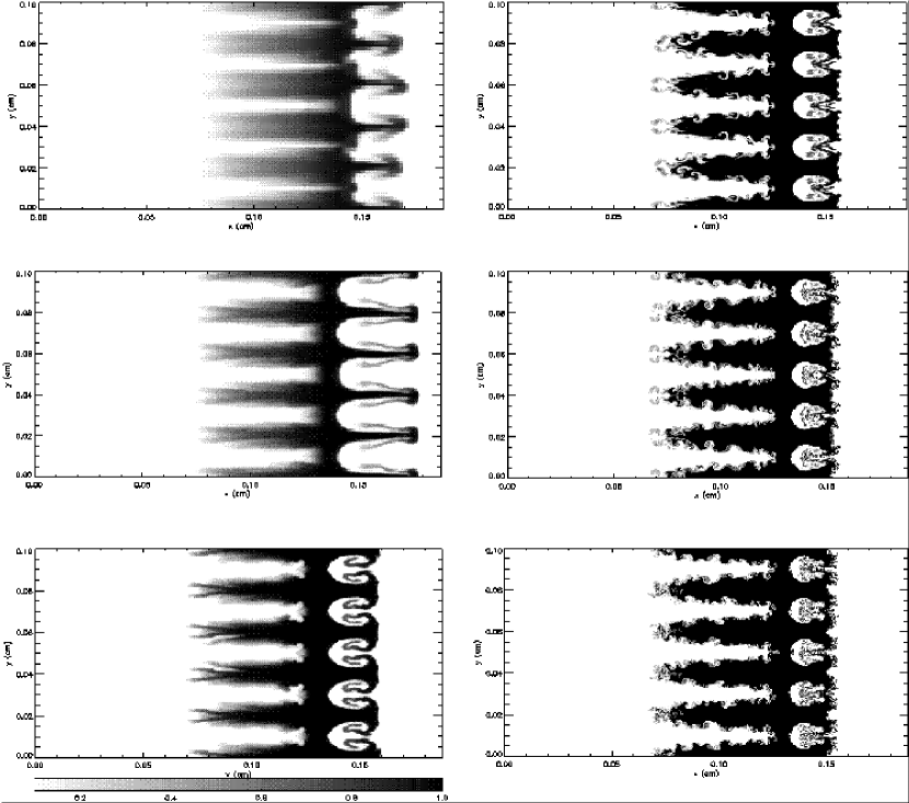
Figure 11: Gray scale images of CH abundance at approximately the time of the late time experimental image, 66.0 ns, from simulations at varying resolutions. The effective simulation resolutions were, top to bottom on left followed by top to bottom on right, 128 $\times$ 64, 256 $\times$ 512, 512 $\times$ 1024, 1024 $\times$ 2048, 2048 $\times$ 4096, corresponding to 4, 5, 6, 7, 8, and 9 levels of adaptive mesh refinement.

We first present the results of a resolution study of the simulation. We performed six simulations from equivalent initial conditions, changing only the maximum mesh resolution. The results of the six simulations are illustrated in Figure 11. As described above, FLASH solves an advection equation for each abundance, allowing us to track the flow of each material with time. Shown are fluid abundances for the CH, the intermediate material, at approximately 66 ns. The abundance is represented by a gray scale, so that the white regions (for which the abundance is zero) to the left and right of the central gray region are Cu and C, respectively. Thus, the CH abundance shows features of both material interfaces, and its evolution shows the behavior of both the spikes of Cu and bubbles of C. The effective simulation resolutions were, top to bottom on left then top to bottom on right, 128 $\times$ 64, 256 $\times$ 512, 512 $\times$ 1024, 1024 $\times$ 2048, 2048 $\times$ 4096, corresponding to 4, 5, 6, 7, 8, and 9 levels of adaptive mesh refinement.

We found that all of the simulations capture the expected bulk properties of the flow; that is, all showed similar spikes of Cu and bubbles of C. The principal differences in the results were in the amount of small scale structure in the flow, with the amount of small-scale structure increasing with resolution. The increasing amount of small scale structure in the simulations should be readily apparent in the panels of the figure. This behavior is expected because the dissipation mechanism in PPM operates on smaller and smaller scales as the resolution is increased. We note that the increasing amount of small-scale structure seen with increasing resolution indicates that these simulations will not demonstrate a converged flow with higher resolution until the turbulent scales are fully resolved; only at this point will we be resolving all the relevant length scales in the problem.

Because, as noted above, we observe increasing amounts of small-scale structure in the simulations with higher resolutions, convergence studies should focus on integrated quantities such instability growth, which may converge. In order to quantify the results, we examined the lengths of the Cu spikes, an integral quantity of the flow that we were best able to accurately measure both in the simulation results and in the experimental results. The spike lengths were measured by averaging the CH abundance in the $y$-direction across the simulation domain then smoothing the resulting one-dimensional array slightly to minimize differences that would occur owing to very small scale structure. The length of the Cu spikes was then determined by the average distance spanned by minimum locations of average abundances 0.05 and 0.9. The results were reasonably robust to the amount of smoothing and threshold values.

The results of testing the convergence of the Cu spike length measurements are shown in Figures 12 and 13. Figure 12 shows percent differences from the highest resolution simulation as functions of time. The trend is that the difference decreases with increasing mesh resolution, with the seven and eight level of adaptive mesh refinement simulations always demonstrating agreement to within five percent. The trend of decreasing difference with increasing mesh resolution demonstrates a convergence of the flow, but it is subject to caveats. We note that the trend does not describe the behavior at all points in time (that is, the percent difference curves sometimes cross each other), and this average measurement is an integral property of the flow and in no way quantifies the differences in small scale structure observed in the abundances. In particular, we note that the difference curve for the simulation with eight adaptive mesh refinement levels crosses the curves of both the seven and six level simulations, suggesting that higher resolution simulations may deviate further from these results and produce degraded agreement with the experiment. Figure 13 shows the Cu spike lengths at approximately the two times of the experimental results, 39.9 and 66.0 ns, vs. number of refinement levels, quantifying the changes of the Cu spike lengths at the times of the experimental results with resolution.

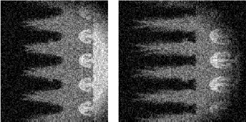
Figure 14: Simulated radiographs from the six level of refinement (effective resolution of 512 $\times$ 256) simulation of the three-layer target experiment. The simulated radiographs were created from the fluid abundances at times corresponding approximately to those of the images from the experiment, 39.9 ns (right) and 66.0 ns (right). Shown are the parts of the simulation domain that match the regions in the experimental results.

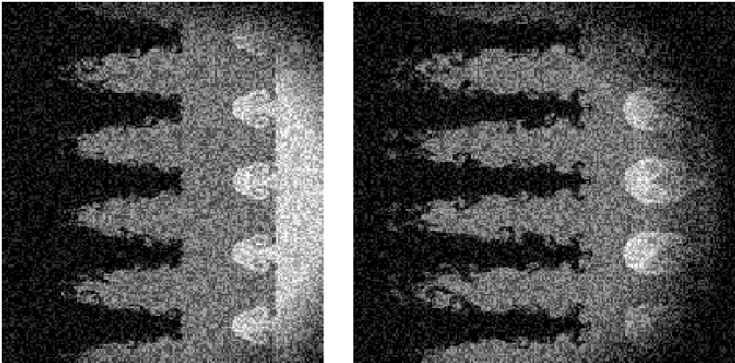
Figure 15: Simulated radiographs from the seven level of refinement (effective resolution of 1024 $\times$ 512) simulation of the three-layer target experiment. The simulated radiographs were created from the fluid abundances at times corresponding approximately to those of the images from the experiment, 39.9 ns (left) and 66.0 ns (right). Shown are the parts of the simulation domain that match the regions in the experimental results.

Figures 14 and 15 show simulated radiographs from two simulations. Both figures show a simulated radiograph at approximately the two times corresponding to the images from the experiment, 39.9 ns (left panel) and 66.0 ns (right panel). The simulation in Figure 14 had six levels of adaptive mesh refinement (an effective resolution of $512\times 256$), while the simulation in Figure 15 had seven levels of refinement ($1024\times 512$). The radiographs were created from the abundances of the three materials. An artificial opacity was assigned to each abundance, Cu having the highest, CH the intermediate, and C the lowest. Then the opacity was applied to intensity from an artificial “beam” that consisted of a circular region that linearly decayed above a certain radius from a point near the center of the simulation domain. In addition, the abundances were de-resolved to match the resolution of the pixels in the images from the experiment and random Poisson ‘noise’ was added to the intensity. Comparison of the simulated radiographs to the radiographs from the experiment show that the simulations captured the bulk behavior of the materials, particularly the growth of Cu spikes and the development of C bubbles.

It is worth noting that the increased amount of small scale structure in the higher resolution simulation is visible in comparing the radiographs even though the images have been de-resolved. From inspection, the amount of small scale structure in the six level simulation appears to agree with that observed in the experiment better than the seven level simulation. This agreement indicates that the amount of viscosity in the experiment is higher than the numerical viscosity of the higher resolution runs. Caution concerning this interpretation is warranted, however, because the experimental radiograph, which is essentially the shadow of the material, will almost certainly fail to capture the true amount of small scale structure. Conclusions regarding the correct amount of small scale structure (and the correct Reynolds number of the flow) must await better diagnostic resolution of the experiments followed by a careful, quantitative comparison with simulation results.

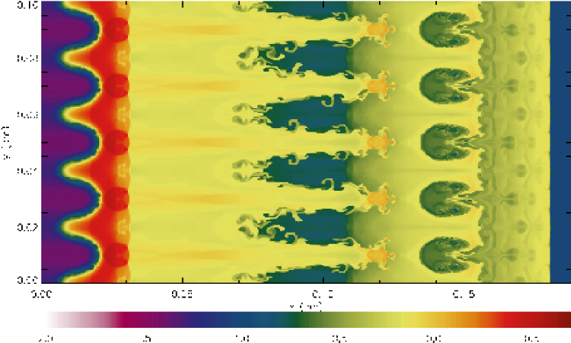
Figure 17: Full resolution image of the log of density from the seven levels of adaptive mesh refinement simulation at approximately the time of the late time experimental result. The spikes of Cu are visible as the reddish-yellow ($\rho\sim 2\ \mathrm{g\ cm^{-3}}$) fingers moving into the less dense ($\rho\sim 0.5\ \mathrm{g\ cm^{-3}}$) CH. The bubbles of C are the dark green ($\rho\sim 0.2\ \mathrm{g\ cm^{-3}}$) regions to the right of, and opposing, the spikes of Cu. The transition from compressed C (rightmost yellowish region) to uncompressed C (blue region on far right) marks the position of the shock, which shows a slight perturbation.

Figure 16 shows the Cu spike length vs. time for the six and seven levels of adaptive mesh refinement simulations. Also shown in the figure are the experimental results. The error bars correspond to $\pm 25\ \mathrm{\mu m}$, the spatial error of the experiment. The width of the symbols marking the experimental results indicates approximately the timing error. The figure shows that the simulations agree well with the experimental results. In addition, inspection of the evolution of the shock as it passes through the CH shows that the shock oscillates as expected from the linear theory of compressible fluids (Dyakov, 1954; Freeman, 1955; Landau & Lifshitz, 1987) and is almost planar when it reaches the CH/C interface. Figure 17 shows the logarithm of density on the entire simulation grid at approximately the time of the late experimental result for the simulation with seven levels of adaptive mesh refinement. In this case, the image is fully resolved (to the resolution of the simulation).

4.2 Rayleigh-Taylor Simulations

The classic Rayleigh-Taylor problem consists of a dense fluid on top of a light fluid in the presence of a gravitational acceleration. The initial configuration is in an unstable equilibrium, and any perturbation of the fluid interface leads to instability growth. In the linear regime, the instability growth rate is proportional to the square root of the perturbation wave number $k$ (Chandrasekhar, 1981). If the interface is sharp, the problem is mathematically ill-posed because the growth rate diverges with large $k$. The simulations we performed began with completely sharp interfaces, but numerical diffusion in the simulation regularizes the problem by increasing the width of the boundary and thereby bounding the growth rate. In experiments, the growth rate is bounded either because surface tension limits the maximum $k$ or because physical diffusion widens the boundary (Duff, Harlow, & Hirt, 1962; Faber, 1995).

Our studies of the Rayleigh-Taylor problem consist of both single- and multi-mode simulations. The validation tests consisted of multi-mode simulations performed from a standard set of initial conditions, allowing for comparison with results of other research groups and experiments. Single-mode simulations allow for testing of convergence of the solutions and are meant to determine the minimum resolution per perturbation wavelength for a converged simulation. This case is of particular interest because it illustrates the difficulty of code validation even for apparently simple laboratory experiments.

In the case of a Rayleigh-Taylor configuration with a multi-mode perturbation, bubble and spike mergers and bubble/spike competition are thought to lead to an instability growth according to a $t^{2}$ scaling law, which may be written as (Youngs, 1994)

$$h_{\mbox{\scriptsize{b,s}}}=\alpha_{\mbox{\scriptsize{b,s}}}gAt^{2}\;,$$ (13)

where $h_{\mbox{\scriptsize{b,s}}}$ is the height of a bubble or spike, $g$ is the acceleration due to gravity, and $A=(\rho_{2}-\rho_{1})/(\rho_{2}+\rho_{1})$ is the Atwood number. $\rho_{1,2}$ is the density of the lighter (heavier) fluid, and $t$ is the time. The coefficient $\alpha$ is a measure of the rate of potential energy release. The initial conditions for the multi-mode simulations consisted of velocity perturbations corresponding to modes 32–64. These initial conditions were adapted from a standard set used by a consortium of researchers. This consortium, known as the Alpha Group, was formed in 1998 by Guy Dimonte for the purpose of investigating the validity of the $t^{2}$ scaling law, and, if it holds, to determine the value of $\alpha$. The study undertaken by the consortium includes both code-to-code comparisons and comparison with experiment (Dimonte et al., 2002).

Recent work on the Rayleigh-Taylor problem by Cook & Dimotakis (2001) and Glimm et al. (2001) indicates a sensitivity of simulation results to initial conditions and numerical diffusion effects. Cook & Dimotakis (2001) performed simulations of the Rayleigh-Taylor instability for the case of incompressible, miscible fluids with a 3:1 density ratio. In this case, the solutions were evolved by the Navier-Stokes equations augmented by a species transport-diffusion equation. Cook and Dimotakis performed three large three-dimensional simulations that differed only in the initial multi-mode perturbation, and their results indicate a sensitive dependence of the growth rates on the initial perturbation. In particular, they found that the growth rates for the perturbation with the smallest characteristic wave number were the fastest, and the growth rates for the perturbation with the largest characteristic wave number were the slowest. In addition, they found that mixing had an even greater dependence on the initial conditions, with their smallest characteristic wave number simulation exhibiting the “largest unmixedness.”

Glimm et al. (2001) performed a study of the effects of numerical diffusion on instability growth rates. The group performed three-dimensional simulations with total variation diminishing (TVD) schemes and with a front tracking scheme. The front tracking results differed from the TVD results by 40%, with the TVD schemes having the smaller rates. The group attributes this difference to the presence of numerical diffusion in the TVD schemes. The TVD simulations were performed with and without an artificial compression scheme to limit mass diffusion, but showed similar results. From these similar results the group concludes that the principal dissipative effect is viscosity, though they note that an alternate explanation is that the artificial compression scheme does not sufficiently control the mass diffusion. It should be mentioned that the initial conditions were not exactly the same for the front tracking and TVD simulations, with the TVD simulations having a lower mode number. Given the results obtained by Cook & Dimotakis (2001), these differences in initial conditions may play a role in the differences found between the TVD and front tracking results, though the effect may be to decrease the differences.

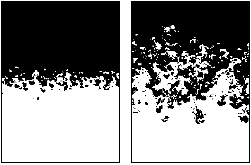
Figure 18: Experimental results from a multi-mode Rayleigh-Taylor experiment performed on the Linear Electric Motor. Shown are bi-level laser-induced fluorescence images from an experiment with Atwood number A = 0.32 at t = 25 ms (left) and 44 ms (right). The dense material ($\rho_{2}=1.43\ \mathrm{g\ cm^{-3}}$) is on the bottom and appears white. The light material ($\rho_{1}=0.73\ \mathrm{g\ cm^{-3}}$) is on the top and appears black. The direction of the acceleration of the experimental capsule was down, providing an effective upward acceleration. The width of the material shown in each panel was 6.2 cm.

The experimental multi-mode Rayleigh-Taylor results come from studies performed by Schneider, Dimonte, & Remington (1998) and Dimonte & Schneider (2000). The experiments investigated the Rayleigh-Taylor instability over a range of density ratios using a variety of sustained and impulsive acceleration histories. The experiments consisted of a sealed plastic fluid container accelerated by the Linear Electric Motor (Dimonte et al., 1996). The diagnostics used for comparison were provided by laser-induced fluorescence, in which a dye is added to the system and excited by a laser beam focused into a sheet propagating upwards through the cell. Images captured with a gated charged-coupled device and 35 mm film cameras allow diagnosis of the internal structure of the mixing zone. Figure 18 shows laser-induced fluorescence images from an experiment with $A=0.32$ and a nominally constant acceleration of $\sim 68$ times the acceleration of gravity on Earth. The images were captured at 25 and 44 ms. The bi-level images shown are made from intensity images by setting the values to zero below and unity above an intensity threshold. The threshold was chosen as $\sim$ 50% to conserve the two fluid volumes. In the images, the lighter material is on the top and appears black, and the heavier material is on the bottom and appears white. Figure 19 shows the bubble and spike magnitudes from the experiment. The resulting values for $\alpha$ were 0.052 for the bubbles and 0.058 for the spikes. Dimonte and Schneider report $\alpha\sim 0.05$ from several experiments with a constant acceleration. These results are in good agreement with earlier experimental work by Youngs (1989).

There are many unknowns that may influence the results of these experiments. There may be unaccounted-for noise in the experiment that can change the actual initial conditions. Since the value of $\alpha$ is thought to be dependent on the power spectrum of the initial perturbation, long wavelength noise in the experiment could make $\alpha$ larger because these modes would dominate the dynamics in the nonlinear regime. This situation will occur if the long wavelength modes never reach the self-similar regime given the length and time scales of the experiment.

In addition, the diagnostics of the experiments may lead to spurious results. For example, because the laser-induced fluorescence method illuminates the mixing zone with a planar sheet of light, this diagnostic can lead to aliasing of long wavelength structures into short wavelength features in the images, thus affecting the interpretation of observed small-scale structures in the mixing zone. Also, because of the dynamic limits on diagnostic resolution, the formation of small-scale structure cannot be completely determined.

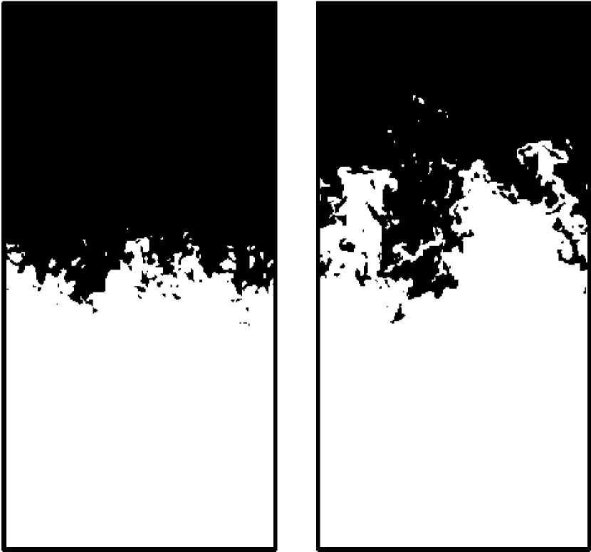
Figure 22: Bi-level cross sections of the multi-mode simulation at $t$ = 8.75 s (left) and 15.5 s (right). The images were produced from cross sections of the heavy fluid abundance in the $x$-$y$ plane at $z$ = 2.5 cm. The images are shown from the same perspective as those from the experiment with the heavy fluid appearing white and the light fluid appearing black and an upward direction of the acceleration.

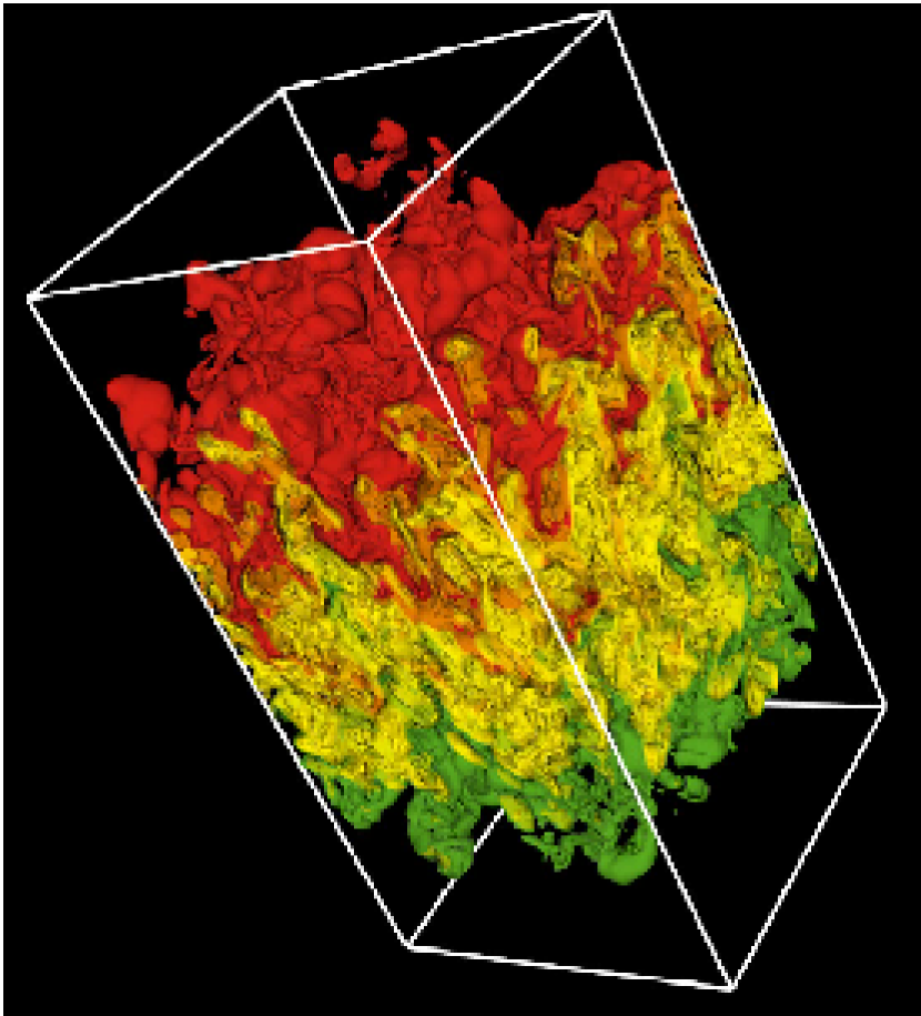
Figure 23: Rendering of the mixing zone of the higher resolution multi-mode Rayleigh-Taylor simulation. Shown is density at a simulation time of 15.5 s. The colors indicate lower density (red), intermediate density (yellow), and higher density (green). Densities higher or lower than those occurring in the mixing zone are transparent. The initial perturbation consisted of modes 32-64, with an effective resolution of $256\times 512\times 256$.

Results of our multi-mode simulations are shown in Figures 20 - 23. The simulations began from a Rayleigh-Taylor configuration with $A=\frac{1}{2}$ ($\rho_{1}=1\ \mathrm{g\ cm^{-3}}$ and $\rho_{2}=3\ \mathrm{g\ cm^{-3}}$) and with $g=2\ \mathrm{cm\ s^{-2}}$. In the simulations, gravity acts in the $y$-direction, and the simulation domain consisted of a $10\times 20\times 10$ cm region, with the fluid interface 10.625 cm above the bottom of the domain. The initial interface displacement perturbation was converted to a velocity perturbation using the linear theory of the Rayleigh-Taylor instability (Chandrasekhar, 1981). In order to completely resolve these initial perturbations, the mesh was forced to be fully resolved in the perturbed region of the simulation domain. This region was 4 cm tall and centered on the initial fluid interface.

Figure 20 shows bubble heights and spike depths for two three-dimensional multi-mode simulations. The effective resolutions of the two simulations in the $(x,y,z)$ directions were $128\times 256\times 128$ and $256\times 512\times 256$. The top two curves are bubble heights, and the lower two curves are spike depths. The bubble heights and spike depths were measured by averaging the density in each $x$-$z$ plane, and comparing the average density profile to the initial density profile, marking the points at which the average density deviated from the initial profile by more than 1%. Results were robust to reasonable changes in this threshold value. The distances shown were measured from the initial fluid interface, and the distance between the two curves from each simulation is the width of the mixing zone. The results show some differences between the two simulations, but both show a predominantly linear growth above a certain point.

Figure 21 shows results from the higher resolution simulation. Shown are bubble and spike magnitudes plotted vs.  $gAt^{2}$ from the higher resolution three-dimensional simulation. The slope of a linear fit to each curve gives $\alpha$, the rate coefficient. The results for $\alpha$, obtained from a linear fit to each curve, were 0.024 and 0.030 for the bubbles and spikes, respectively. If we neglect the first five seconds as being part of a different stage of evolution than the merger-dominated regime that gives the $t^{2}$ behavior and look at the slopes, we find lower results for $\alpha$, 0.021 and 0.026.

Figure 22 allows for visual comparison of the structure of the mixing zone of the higher resolution simulation to that of the experiment. Because the multi-mode simulations were not designed to match the experiments, (i.e. different Atwood numbers, accelerations, and geometry), we may make only a qualitative comparison. Figure 22 shows bi-level images of the simulation at $t$ = 8.75 s. (left panel) and $t$ = 15.5 s. (right panel). The images were created from the heavy fluid abundance in the $x$-$y$ plane at $z$ = 2.5 cm by setting the values to zero below and unity above an abundance of 0.5. As with the experimental results, the dense fluid is on the bottom and appears white, and the light fluid is on the top and appears black. The early time was chosen to match the proportion of evolution as that of the early time in the experimental images. Figure 23 is a rendering of density from the higher resolution simulation. Shown is the mixing zone, with well-developed bubbles and spikes. The colors indicate lower density (red), intermediate density (yellow), and higher density (green). The higher and lower density material above and below the mixing zone is transparent. As illustrated in these figures, the higher resolution multi-mode simulation shows a very similar structure to the experiments. Our results indicate $\alpha\leq 0.03$, however, which is not in good agreement with the experiments and indicates the presence of some systematic error. Other research groups in the consortium using Eulerian hydrodynamics methods report similar results, although groups using other methods report different results. Results of consortium studies will appear in publications of the Alpha Group (Dimonte et al., 2002).

Because our multi-mode simulations did not agree well with the experimental results, we initiated a study of single-mode instabilities to further investigate mesh resolution effects. The single-mode simulations all began from initial conditions consisting of $A=\frac{1}{3}$ ($\rho_{1}=1\ \mathrm{g\ cm^{-3}}$ and $\rho_{2}=2\ \mathrm{g\ cm^{-3}}$) with $g=1\ \mathrm{cm\ s^{-2}}$. The initial perturbation consisted of a sinusoidal vertical velocity perturbation of 2.5% of the local sound speed, with the horizontal components chosen to make the initial velocity field divergence-free, corresponding to the near-incompressible nature of the experiments. The simulation domains were 0.25 cm $\times$ 1.5 cm for the two-dimensional simulations and 0.25 cm $\times$ 1.5 cm $\times$ 0.25 cm for the three-dimensional simulations. As with the multi-mode simulations, the grid was forced to be fully resolved in the region of the initial perturbation.

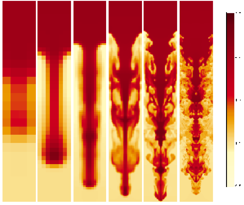
Figure 25: Plots of density (in a plane through the center of the domain) from three-dimensional single-mode instability simulations at 3.1 s of evolution time. The effective resolutions for the panels are, from left to right, $\lambda=$ 4, 8, 16, 32, 64, and 128 grid points. In the images, the value of each computational zone was determined from the zone averaged values and no interpolation was done. The effect is that one sees the zones as a series of squares of uniform color. This effect is obvious in the panels from the lower resolution simulations.

Results from these simulations are shown in Figures 24 - 26. Figure 24 shows plots of bubble height and spike depth for two simulations, one two-dimensional (dashed lines) and one three-dimensional (solid lines), from equivalent initial conditions. The top two curves are bubble heights, and the lower two curves are spike depths. The effective simulation resolutions are 128 $\times$ 768 (2-d) and 128 $\times$ 768 $\times$ 128 (3-d). In these calculations, the bubble heights and spike depths were measured by tracking the advection of each fluid and recording the positions of 99% and 1% abundances. The distances shown were measured from the initial fluid interface. The distance between the two curves from each simulation represents the width of the mixing zone. The results indicate that instability growth rates in three-dimensional simulations are larger than those found in the equivalent two-dimensional simulations as was observed by Kane et al. (2000) (see also Young et al., 2001, for an incompressible comparison).

In addition, we find that obtaining a reasonably converged estimate of the growth rate requires at least 25 grid points per wavelength of the perturbation, that grid noise seeds small-scale structure, and that the amount of small-scale structure increases with resolution. As noted with the results of the laser-driven shock experiments, this behavior is expected because the dissipation mechanism in PPM operates on smaller and smaller scales as the resolution is increased. Another result is that poorly-resolved simulations exhibit a significant amount of mixing due to numerical diffusion. Figure 25 illustrates these results. The panels are images of density after 3.1 s of evolution for six three-dimensional simulations of increasing resolution from the same initial conditions. Shown in each panel is a cross-section of the simulation volume in the $y$-$z$ plane. In the simulations, the acceleration due to gravity acts in the $y$-direction. The effective resolutions are, from left to right, $\lambda$ = 4, 8, 16, 32, 64, and 128 grid points. The mixing due to numerical diffusion is readily visible in the lower resolution results, as is the trend toward increasing amounts of small-scale structure with resolution. We note that our “metric” for measuring resolution in terms of grid point per wavelength assumes square or cubic mesh cells. Adding resolution along the direction of gravity without adding resolution in directions perpendicular to gravity would decrease the amount of mixing due to numerical diffusion without changing the number of grid points per wavelength.

It is worth noting that the instability growth rate, an integral property of the flow, does not converge with increasing mesh resolution in the case of the single-mode Rayleigh-Taylor instability. Figure 26 plots the spike length vs.  wavelength of the perturbation ($\lambda$) measured in number of grid points. The greatest spike length is not found at the highest resolution. We attribute the decrease in instability growth rate found in the highest resolution to the increased amount of small-scale structure. Further studies of the single-mode Rayleigh-Taylor and the role of small scale structure are underway, and complete results will appear in Calder et al. (2002).

4.3 A Note on Convergence

As described above, our hydrodynamics model is inviscid. Making this model solvable requires a dissipative mechanism, but such a mechanism does not guarantee convergence. In our case, because the PPM dissipation mechanism does not include a fixed damping length scale, there can always be fluid motion on the smallest scale we resolve. If those motions affect the bulk properties, then even a measure of these bulk properties will not converge with increasing mesh resolution. There exist differing opinions in the literature regarding the effects of the PPM dissipation mechanism on simulation results.

Porter & Woodward (1994)(see also Porter & Woodward, 2000) investigated numerical diffusion of PPM in two dimensions. They found that the numerical viscosity in PPM depends on velocity of the flow and the mesh resolution. Recent numerical work by Sytine (2000) performed convergence tests for PPM and Navier-Stokes simulations of homogeneous compressible turbulence in three dimensions. By studying kinetic energy, enstrophy, and energy power spectra, they found convergence of the PPM and Navier-Stokes solutions to the same limit.

Caution is warranted, however, about the future use of PPM for simulating subsonic turbulent flows. Garnier et al. (1999), in a study of decaying isotropic turbulence, found that the flow suffered from excessive numerical damping on small length scales and that not all of the properties of the turbulent flow were correctly reproduced. This dissipation makes shock-capturing schemes poor choices for use with explicit subgrid-scale models. Also, Xu & Li (2001) found that the dissipation in Godunov methods depends on the character of the flow and the mesh configuration, and is not always consistent with the Navier-Stokes viscous terms. Transonic turbulent flows, however, where viscosity is not the primary dissipative mechanism, remains an open research question.

Clearly, the limitations of present computing resources prevent us from adequately resolving both the laser experiments and fully-developed turbulent flows. The simulations we are capable of performing, however, are approaching the resolution required to resolve these flows. Moore’s Law (Moore, 1965) would indicate that computing resources for these types of flow may be available fairly soon. At that point, experiments such as the laser-driven fluid dynamics experiments (particularly with another generation of growth and improvements in diagnostics), could serve as validation test beds for simulations of turbulent flows. Those astrophysical flows with dramatically larger Reynolds numbers are not likely to be resolved in the foreseeable future. The lessons learned in modeling turbulent flows, though, should allow for the improvement of hydrodynamic methods and the development of appropriate subgrid models, making astrophysical simulations more realistic and accurate. Further, if as we increase the resolution of our simulations we eventually will converge with Navier-Stokes flows as indicated by Sytine (2000), we may be able to determine the correct amount of small scale structure for these flows and thereby answer some of the unanswered questions in this study.

5 Conclusions

In this paper, we presented the results of our efforts at verification and validation of FLASH, our astrophysical simulation code. We presented the results of new verification tests and the results of two validation tests in which we were able to carefully compare our simulation results to experimental results. These tests served to increase our understanding of the physics relevant to the problems of interest, to improve our simulation techniques, and to build confidence in our results.

5.1 Verification

The verification tests we performed for this study indicate that the PPM hydrodynamics module is performing as expected. Advection tests on a uniform mesh showed slightly better than second order convergence of the error with mesh resolution. The PPM module, on a uniform mesh, propagated a sound wave for one period with approximately second order accuracy, and a shock wave, as expected, to first order. In the case of a shock wave on an adaptive mesh, the code showed the expected first-order convergence as well. The code was able to hold a standing shock steady for several times steps, also, indicating the Riemann solver is working correctly.

The material equation of state, as well as the hydrodynamic solver, must be well known and well behaved in order to obtain a meaningful comparison with experiments. Verification testing of a test equation of state resulted in establishing a procedure for testing consistency and quantifying the results. This procedure will allow us to quickly test new equations of state as we develop additional physics modules and address new astrophysical problems.

5.2 Validation

The results of simulating laser-driven shock experiments show that we can capture the bulk properties of the flow, including the morphological properties of the resolvable structures. We observed the expected instabilities at the two material interfaces that grew with time during the course of the simulations. We performed a mesh resolution study that in general showed convergence of instability growth at the material interfaces. The resolution study did not completely demonstrate convergence, though, because the amount of small scale structure present in the simulations increased with resolution as may be seen by a visual inspection of the results (Figure 11). We attribute this increasing amount of small scale structure to the fact that the amount of numerical dissipation in our hydrodynamics method decreases with increasing resolution. Visual inspection of the experimental results and our simulated radiographs suggested that a simulation with six levels of adaptive mesh refinement better matched the observed small scale structure. We note, though, that the correct amount of small scale structure in the experiments is not likely captured in the experimental diagnostics because of resolution limits and because the radiograph produces a two-dimensional shadowgraph of a three-dimensional experiment, possibly averaging out small structures.

Measurement of the lengths of the spikes allowed us to quantify the results of the simulations, and we found that simulations with seven and eight levels of adaptive mesh refinement agreed to within 5% of the highest resolution (nine levels) simulation at all times during the evolution (Figure 16). Complete convergence is prohibited by the growth in small-scale structure with increasing resolution.

The spike lengths at intermediate resolutions match the experimental results very well, falling within the experimental errors. We interpret these as an important calibration result that indicates that six and seven levels of adaptive mesh refinement are appropriate for two-dimensional simulations of these particular experiments. In addition, the simulations showed that the shock propagating through the corrugated material interface develops a perturbation that oscillates and becomes planar at the second interface, as expected from theory. We also observed the expected imprinting of the perturbation on this second interface.

For this validation problem, comparison between simulation and experiment is limited by the diagnostic resolution of the experiments and the amount of physics included in the simulations. Improvements to experimental diagnostics will be made in the next generation of laser experiments, and improvements to the simulations could be made by inclusion of a more realistic material equation of state, adding the walls of the shock tube, and modeling the laser-driven energy deposition process. Absent these improvements, we cannot conclude that the good agreement of our results with the experiment completely validates the simulations.

The results of simulations of a single-mode Rayleigh-Taylor instability demonstrated the effect of resolution and dimensionality on growth rates. The single-mode simulations established that $\sim$ 25 grid points per mode are required for a reasonable estimate for the growth rate. This calibration result suggests a minimum resolution for simulations involving the Rayleigh-Taylor instability with our code. This required resolution may make complete simulations of many problems prohibitively expensive at the present time. We confirm previous findings (Kane et al., 2000; Young et al., 2001) that instability growth rates in three-dimensional simulations are larger than those found in the equivalent two-dimensional simulations, which indicates limits on results from two-dimensional models of astrophysical phenomena. The single-mode simulations also showed that, as with the laser-driven shock simulations, one sees structure formation at smaller and smaller scales as resolution is increased. The result is that increasing resolution will not necessarily produce a converged flow. Further, the single-mode simulations also showed that small scale structure in highly resolved simulations can have an effect on integral properties of the flow, in this case instability growth rates.

Our multi-mode Rayleigh-Taylor instability simulations, like the simulations of the laser experiment, show that the code results agree with the observed bulk properties of the flow: we observe a mixing zone that is very similar in structure to that of the experiment. Our simulations do not, however, agree well with the experimental rate coefficient, $\alpha$; our results are systematically lower. This difference could be due to limitations of either the simulations or the experiments. The experimental initial conditions, which strongly effect the growth rate, are poorly characterized. Further, limitations on experimental diagnostics may distort measured growth rates and mixing.

The simulations, on the other hand, may have been under-resolved. In our low-resolution simulation, most of the power in the initial conditions was in modes which were resolved with only $2$–$4$ grid points; in light of our single-mode results, this is far too low. Increasing the resolution to resolve these modes with $4$–$8$ points increases the observed growth rate, in (somewhat) closer agreement with experimental results.

5.3 Evaluation of V&V Results

The principal conclusions we draw from our efforts are that validation of an astrophysical simulation code is a difficult process and that the process led us to unanticipated questions. The verification tests we performed allowed for a careful quantitative study of the accuracy and convergence rates of FLASH. The exercise proved useful in a variety of ways, not the least of which was developing techniques for accurately comparing the results of our simulations to accepted answers. The validation tests we performed, while they did not conclusively validate the simulations, provided insight into the many issues involved in numerical modeling, and served to calibrate the code and build confidence in our results.

V&V testing allows for an assessment of error in the code and progress in building confidence in the results. The process is limited, though. Analytic solutions are typically available only for simple problems, which may not serve as a strenuous tests of a particular code. Convergence studies, though essential, do not imply that the converged answer is correct. Code-to-code comparisons are another useful tool; they can be more probing than analytic solutions, and can shed insight into the behavior of different methods. But again, similar answers do not imply correctness.

Comparing numerical and experimental results is also difficult. Nonlinear systems typically have exponential sensitivity to initial conditions, so that any unmodeled initial perturbation in the system can greatly affect the results. Experimental results may be limited, noisy measurements of a poorly-characterized but real physical situations, while the numerical results may be complete diagnostics of the situation derived by a model of dubious applicability. Comparisons must, therefore, rely on choosing features which are obtainable from both results, yet sensitive enough to the physics of interest that comparing the features is a strong probe of the model and numerics. The complexity of this procedure means that doing it well requires feedback between the computational and experimental researchers, with all parties improving techniques and performing multiple runs. The computational simulations may be very expensive, however, and performing relevant experiments is a costly and difficult process. This makes it hard to improve results and demonstrate reproducibility.

As our stated goal in this work was validating an astrophysical simulation code, the assumptions in the models and their applicability to both terrestrial and astrophysical flows warrants discussion. Our numerical models did not have an explicit viscosity. We saw, however, that the effects of numerical dissipation cannot be avoided in simulations. Other physical processes that may play a role but are not included in the models include surface tension, species diffusion, and thermal diffusion. With only Euler’s equations, it is impossible to adjust the relevant dimensionless numbers (Schmidt, Reynolds, Rayleigh, and Prandtl numbers, for example) to match the correct properties of the fluid.

Our use of models without an explicit viscosity resulted in an increasing amount of small scale structure observed with increasing resolution in simulations of both validation problems. As mentioned above, limits on diagnostic resolution prevent us from determining the correct amount of small scale structure in both validation experiments. Were the experimental diagnostics better, we could incorporate physically-motivated terms for viscosity, surface tension, or diffusion into the equations we evolve and calibrate their magnitudes until we obtain a converged flow with the correct amount of small scale structure. Proceeding in this manner (as well as including a physically-motivated equation of state) would help us validate our simulations of these and similar terrestrial experiments, but would be of little use in the astrophysical case, where viscosity and surface tension play no dynamic role.

Even with better diagnostics these types of experiments can only further validate the code if we model additional physics that are not relevant to the astrophysical problems of interest. As we mentioned above, flows within stars are expected to have a Reynolds number greater than 10⁹, for which the viscosity-free Euler equations are a better approximation, but such flows are impossible to achieve either in the laboratory or in current simulations. Therefore, we conclude that the terrestrial experiments we have simulated have served to build confidence in the hydrodynamics module in FLASH, but that there are certainly still limits on the strength of statements we can make about the validity of FLASH simulations of laboratory experiments.

We end by repeating a point from our introduction, namely that verification and validation can determine only if a code returns an incorrect answer. Verification and validation cannot prove that a theoretical result, either numeric or analytic, is correct. By doing a sufficient number of tests, however, one can significantly increase one’s confidence in the results. Our efforts at validation, although they have presented many challenges and led to new questions such as the effect of small scale structure on bulk properties of flows, have increased our confidence in the simulations produced by FLASH.

Figure 1: Schematic of the ranges of validity of a simulation code. The goal of computational science is to accurately describe Nature with a theory implemented by a numerical method. In practice, there is a desired range of Nature that is to be described, consisting of the problems of interest. The goal of validation is to confirm that the range of actual validity of the code and models adequately describes the desired range of validity. Verification is testing that a numerical implementation accurately represents the model. In this schematic, validation may be thought of as probing the range of actual validity, represented by the circle labeled range of actual validity. Verification may be thought of as confirming the mapping between the theory and numerics circles.

Figure 2: Plot of L2 norm of the density error vs. mesh spacing for a simple advection test consisting of a Gaussian density pulse propagating at a constant velocity across the mesh. The simulation used full PPM including contact steepening. The sudden decrease in error for resolutions below $\approx 10^{-3}$ is due to the narrow pulse being sufficiently well-resolved that contact steepening was no longer applied. The different behavior of the density error at the lowest resolutions occurs because the initial conditions are not adequately resolved.

Figure 3: Plot of L2 norm of the density error vs.  mesh spacing for a simple one-dimensional advection test consisting of a Gaussian density pulse propagating at a constant velocity across the mesh. Contact steepening was turned off to make sure we understood the feature of the curve in Figure 2. The different behavior of the density error at the lowest resolutions occurs because the initial conditions are not adequately resolved.

Figure 4: Plot of L2 norm of the density error vs. mesh spacing for one-dimensional simulations of a sinusoidal sound wave propagating across the simulation domain.

Figure 5: Plot of L2 norm of the density error vs. mesh spacing for the Sod shock tube test.

Figure 6: Plot of L2 norm of the density error vs. minimum mesh spacing for the Sod shock tube test performed on an adaptive mesh. The maximum mesh spacing of each simulation was that of the least-resolved uniform mesh simulation.

Figure 7: Plot of L2 density error vs. mesh spacing for a two-dimensional advection test consisting of an isentropic vortex propagating diagonally across the simulation mesh. Shown are results from two sets of simulations, one with full PPM and one with non-linear steepening turned off. A power-law fit to the curves gave exponents of 2.13 for the default curve and 2.03 for the discontinuity-free curve.

Figure 8: Results of testing the electron/positron equation of state. The panels from left to right show the results with 5, 7, and 9 Riemann solver iterations. Each panel represents the density-temperature plane in log-log scale, with density on the x-axis and temperature on the y-axis. The density ranged from $10^{-30}$ to $10^{-19}\ \mathrm{g\ cm^{-3}}$ and the temperature ranged from $10^{4}$ to $10^{11}$ K. The gray scale indicates a relative error between $10^{-17}$ (white) and $10^{-1}$ (black).

Figure 9: Results of the 3-layer target experiment. Shown are side-on X-ray radiographs at 39.9 ns (left) and 66.0 ns (right). The long, dark “fingers” are spikes of expanding Cu, and the horizontal band of opaque material to the right of the spikes of Cu is the brominated plastic tracer showing the imprinted instability growth at the plastic-foam interface.

Figure 10: Schematic of the 3-layer target simulation initial conditions. Shown are the locations of the three materials, Cu, CH, and C, the shock, and the details of the sinusoidal perturbation of the Cu-CH interface. The schematic is not to scale.

Figure 12: Percent difference of the Cu spike lengths from those of the highest resolution (9 levels of adaptive mesh refinement) simulation vs. time. The percent differences are from the lower resolution simulations of 4, 5, 6, 7, and 8 levels of adaptive mesh refinement. We note that the convergence is not perfect. The curve from the 8 level of refinement simulation crosses those of the 6 and 7 level of refinement simulations, indicating a higher percent difference.

Figure 13: Cu spike length vs. adaptive mesh refinement level. Shown are the spike lengths at the two times corresponding to those of the experimental results from all of the simulations. The percent differences shown in Figure 12 were calculated at many times in the simulations. This figure illustrates how the spike length changed with resolution at the two times of the experimental results.

Figure 16: Cu spike length vs. time. The curves are from simulations at 6, 7, 8, and 9 levels of refinement simulations (effective resolutions of 256 $\times$ 512, 512 $\times$ 1024, 1024 $\times$ 2048, 2048 $\times$ 4096), and the points with error bars are results from the experiment. The error bars represent $\pm 25\ \mathrm{\mu m}$, and the width of the symbols represents the timing error.

Figure 19: Plot of distance vs.  $gAt^{2}$ from a multi-mode Rayleigh-Taylor experiment performed on the Linear Electric Motor. Shown are the magnitudes of bubble height and spike depth as functions of the product of acceleration ($g$), Atwood number ($A$), and the time squared ($t^{2}$). The slope of each curve equals $\alpha$, the rate coefficient. For this experiment, fitting straight lines to the curves produced $\alpha=0.052\mbox{ and }0.058$ for the bubbles and spikes, respectively.

Figure 20: Plot of distance vs. time from two three-dimensional multi-mode simulations. Shown are bubble heights (the two top curves) and spike depths (the two lower curves) as measured from the initial fluid interface. The simulations had effective resolutions of $128\times 256\times 128$ and $256\times 512\times 256$.

Figure 21: Plot of distance vs.  $gAt^{2}$ from the higher resolution ($256\times 512\times 256$) three-dimensional simulation. Shown are the magnitudes of bubble height and spike depth as functions of the product of acceleration ($g$), Atwood number ($A$), and the time squared ($t^{2}$). The slope of each curve equals $\alpha$, the rate coefficient. For this simulation, fitting straight lines to the entire curves produced $\alpha=0.024\mbox{ and }0.030$ for the bubbles and spikes, respectively. If the first five seconds of evolution are neglected to eliminate the parts of the curves with a rapidly changing slope, a straight line fit yields $\alpha=0.021\mbox{ and }0.026$. The thin vertical line at $gAt^{2}=25$ marks $t=5$ s.

Figure 24: Bubble heights and spike depths vs.  time for two-dimensional and three-dimensional simulations of single-mode Rayleigh-Taylor instabilities. The top two curves are bubble heights, and the lower two curves are spike depths. Each distance was measured from the initial fluid interface. The effective resolutions were 128 $\times$ 256 (2-d) and 128 $\times$ 256 $\times$ 128 (3d).

Figure 26: Spike magnitude vs. resolution from the single-mode instability simulations. The points making the curve correspond to the spike magnitudes from the simulations for which density plots are presented in Figure 26.

Table 1: Percentages of the failures at several required accuracies for the the electron/positron equation of state and 5 Riemann solver iterations.

required accuracy	cases failed [%]
$10^{-1}$	0.02
$10^{-2}$	6.7
$10^{-3}$	21
$10^{-4}$	34
$10^{-5}$	43
$10^{-6}$	49

References

- AIAA (1998) AIAA 1998, Guide for the Verification and Validation of Computational Fluid Dynamics Simulations (AIAA Report G-077-1998; Reston, VA: American Institute of Aeronautics and Astronautics)
- Alexakis, Young, & Rosner (2002) Alexakis, A., Young, Y.-N., & Rosner, R. 2002, Phys. Rev. E, 65, 026313
- Alexakis, et al. (2002) Alexakis, A., et al. 2002, in prep.
- Arnett, Fryxell, & Müller (1989) Arnett, D., Fryxell, B., & Müller, E. 1989, ApJ, 341, L63
- Bazán & Arnett (1998) Bazán, G., & Arnett, D. 1998, ApJ, 496, 316
- Birn, et al. (2001) Birn, J., et al. 2001, J. Geophys. Res., 106 A3, 3715
- Blinnikov & Khokhlov (1987) Blinnikov, S. I., & Khokhlov, A. M. 1987, Sov. Astron. Lett., 13, 364
- Blottner (1990) Blottner, F. G. 1990, AIAA Journal of Spacecraft and Rockets, 27, No. 2, 113
- Boehly (1995) Boehly, T. R., et al. 1995, Rev. Sci. Instrum. 66, 508
- Boehm (1981) Boehm, B.W. 1981 Software Engineering Economics, Prentice-Hall
- Boisseau et al. (1996) Boisseau, J. R., Wheeler, J. C., Oran, E. S., & Khokhlov, A. M. 1996, ApJ, 471, L99
- Boris & Book (1973) Boris, J. P., & Book, D. L. 1973, J. Comput. Phys., 11, 38
- Bradley (1998) Bradley, D. K., et al. 1998, Phys. Plasmas 5, 1870
- Burrows, Hayes, & Fryxell (1995) Burrows, A., Hayes, J., & Fryxell, B. 1995, ApJ, 450, 830
- Calder et al. (2000) Calder, A. C., et al. 2000, in Proc. Supercomputing 2000, (IEEE Computer Soc.) http://sc2000.org/proceedings/
- Calder et al. (2002) Calder, A. C., et al. 2002, in prep.
- Chandrasekhar (1981) Chandrasekhar, S. 1981, Hydrodynamic and Hydromagnetic Stability (New York: Dover)
- Colgate & White (1966) Colgate, S. A., & White, R. H. 1966, ApJ, 143, 626
- Colella & Glaz (1985) Colella, P., & Glaz, H. M. 1985, J. Comput. Phys., 59, 264
- Colella & Woodward (1984) Colella, P., & Woodward, P. 1984, J. Comput. Phys., 54, 174
- Cook & Dimotakis (2001) Cook, A. W., & Dimotakis, P. E. 2001, J. Fluid. Mech., 443, 69
- Dimonte et al. (2002) Dimonte, G., et al. 2002, in prep.
- Dimonte & Schneider (2000) Dimonte, G., & Schneider, M. 2000, Phys. Fluids A, 12, 304
- Dimonte et al. (1996) Dimonte, G., Morrison, J., Hulsey, S., Nelson, D., Weaver, S., Susoeff, A., Hawke, R., Schneider, M., Batteaux, J., Lee, D., & Ticehurst, J. 1996, Rev. Sci. Instrum., 67, 302
- Dimotakis (2000) Dimotakis, P. E. 2000, J. Fluid Mech., 409, 69
- Duff, Harlow, & Hirt (1962) Duff, R. E., Harlow, F. H., & Hirt, C. W. 1962, Phys. Fluids, 4, 417
- Dyakov (1954) Dyakov, S. P. 1954, ZhETF 27, 288 in Russian.
- Emery (1968) Emery, A. F. 1968, J. Comput. Phys. 2, 306
- Faber (1995) Faber, T. E. 1995, Fluid Dynamics for Physicists (Cambridge: Cambridge Univ. Press), 293
- Forester (1977) Forester, C. K. 1977, J. Comput. Phys., 23, 1
- Freeman (1955) Freeman, N. C. 1955, Proc. Roy. Soc. A, 228, 341
- Frenk et al. (1999) Frenk, C. S., et al. 1999, ApJ, 525, 554
- Fryxell & Woosley (1982) Fryxell, B. A., & Woosley, S. E. 1982, ApJ, 258, 733
- Fryxell, Müller, & Arnett (1989) Fryxell, B. A., Müller, E., & Arnett, D. 1989, Hydrodynamics and Nuclear Burning (MPI Astrophys. Rep. 449; Garching: MPI Astrophys.)
- Fryxell (1994) Fryxell, B. 1994, in Numerical Simulations in Astrophysics, ed. J. Franco, S. Lizano, L. Aguilar, & E. Daltabuit (Cambridge: Cambridge Univ. Press), 175
- Fryxell et al. (2000) Fryxell, B., et al. 2000, ApJS, 131, 273
- García-Senz, Bravo, & Woosley (1999) García-Senz, D., Bravo, E., & Woosley, S.E. 1999, A&A, 349, 177
- Garnier et al. (1999) Garnier, E., et al. 1999, J. Comput. Phys. 153, 273
- Gehrz et al. (1998) Gehrz, R. D., Truran, J. W., Williams, R. E., & Starrfield, S. 1998, PASP, 110, 3
- Glasner & Livne (1995) Glasner, S. A., & Livne, E. 1995, ApJ, 445, L149
- Glasner, Livne, & Truran (1997) Glasner, S. A., Livne, E., & Truran, J. W. 1997, ApJ, 475, 754
- Glimm et al. (2001) Glimm, J., Grove, J. W., Li, X. L., Oh, W., & Sharp, D. H. 2001, J. Comput. Phys., 169, 652
- Godunov (1959) Godunov, S. K. 1959, Mat. Sbornik, 47, 271
- Godunov (1961) Godunov, S. K., Zabrodin, A. V., & Prokopov, G. P. 1961, U.S.S.R. Computational Math. and Math. Phys., 1, 1187
- Gropp, Lusk, & Skjellum (1999) Gropp, W., Lusk, E., & Skjellum, A. 1999, Using MPI: Portable Parallel Programming with the Message Passing Interface, 2nd ed. (Cambridge: MIT Press)
- Hansen & Van Horn (1975) Hansen, C. J., and Van Horn, H. M. 1975, ApJ, 195, 735
- Hillebrandt & Niemeyer (2001) Hillenbrandt, W., & Niemeyer, J. C. 2001, ARA&A, in press
- Heger, Langer, & Woosley (2000) Heger, A., Langer, N., & Woosley, S. E. 2000, ApJ, 528, 368
- Herant et al. (1994) Herant, M., Benz, W., Hix, W. R., Fryer, C. L., & Colgate, S. A. 1994, ApJ, 435, 339
- Holmes et al. (1999) Holmes, R. L., Dimonte, G., Fryxell, B., Gittings, M. L., Grove, J. W., Schneider, M. S., Sharp, D. H., Velikovich, A. L., Weaver, R. P., & Zhang, Q. 1999, J. Fluid. Mech., 389, 55
- Huang & Greengard (2000) Huang, J., & Greengard, L. 2000, SIAM J. Sci. Comp., 21, 1551
- Janka & Müller (1996) Janka, H.-Th., & Müller, E. 1996, A&A, 306, 167
- Jeans (1902) Jeans, J. H. 1902, Phil. Trans. Roy. Soc. (London), 199, 1
- Kane et al. (2000) Kane, J., Arnett, D., Remington, B. A., Glendinning, S. G., Bazán, G., Müller, E., Fryxell, B. A., Teyssier, R. 2001, ApJ, 528, 989
- Kane et al. (2001) Kane, J. O., Robey, H. F., Remington, B. A., Drake, R. P., Knauer, J., Ryutov, D. D., Louis, H., Teyssier, R., Hurricane, O., Arnett, D., Rosner, R., & Calder, A. 2001, Phys. Rev. E, 63, 055401 (R)
- Keil, Janka, & Müller (1996) Keil, W., Janka, H.-Th., & Müller, E. 1996, ApJ, 473, L111
- Kercek, Hillebrandt & Truran (1998) Kercek, A., Hillebrandt, W., & Truran, J. W. 1998, A&A, 337, 379
- Kercek, Hillebrandt, & Truran (1999) Kercek, A., Hillebrandt, W., & Truran, J. W. 1999, A&A, 345, 831
- Kifonidis et al. (2000) Kifonidis, K., Plewa, T., Janka, H.-Th., & Müller, E. 2000, ApJ, 531, L123
- Khokhlov (2001) Khokhlov, A. M. 2001, ApJ, submitted (astro-ph/0008463)
- Khokhlov (1995) Khokhlov, A. M. 1995, ApJ, 449, 695
- Khokhlov, Oran, & Wheeler (1997) Khokhlov, A. M., Oran, E. S., & Wheeler, J. C. 1997, ApJ, 478, 678
- Lai (2000) Lai, D. 2000, ApJ, 540, 946
- Lamb (2000) Lamb, D. Q. 2000, ApJS, 127, 395
- Lamb, Miller, & Taam (1996) Lamb, D. Q., Miller, M. C., & Taam, R. E. 1996, BAAS, 28, 960
- Lamb, Pethick, & Pines (1973) Lamb, F. K., Pethick, C. J., and Pines, D. 1973, ApJ, 184, 271
- Landau & Lifshitz (1987) Landau, L. D., & Lifshitz, E. M. 1987, Fluid Mechanics, 2nd ed. (Oxford: Pergammon Press)
- Landen, et al. (2001) Landen, 0. L., et al. 2001, Rev. Sci. Instrum., 72, 627
- Larson & Lane (1994) Larson, J. T., & Lane, S. M. 1994, J. Quant. Spect. Rad. Trans. 51, 179
- Livne (1993) Livne, E. 1993, ApJ, 412, 634
- Lewin, van Paradijs, & Taam (1993) Lewin, W. H. G., van Paradijs, J., & Taam, R. E. 1993, Space Sci. Rev., 62, 223
- Lindl (1998) Lindl, J. D. 1998 Inertial confinement Fusion (Springer-Verlag: New York), 54
- Livio (1994) Livio, M. 1994, Mem. Soc. Astron. Ital., 65, 49
- Livio & Truran (1990) Livio, M., & Truran, J. W. 1990, in Nonlinear Astrophysical Fluid Dynamics, ed. J. R. Buchler & S. T. Gottesman, (New York: New York Academy of Sciences), 126
- Lyon & Johnson (1992) Lyon, S. P., & Johnson, J.D. 1992, Los Alamos report LA-UR-92-3407
- MacNeice et al. (1999) MacNeice, P., Olson, K. M., Mobarry, C., de Fainchtein, R., & Packer, C. 1999, NASA Technical Report CR-1999-209483
- MacNeice et al. (2000) MacNeice, P., Olson, K. M., Mobarry, C., de Fainchtein, R., & Packer, C. 2000, Comput. Phys. Commun., 126, 330
- Majda (1984) Majda, A. 1984, Compressible Fluid Flow and Systems of Conservation Laws in Several Space Variables (New York: Springer-Verlag), 7
-
Martin & Cartwright (1996)
Martin, D. F., & Cartwright, K. 1996,
http://seesar.lbl.gov/anag/staff/martin/AMRPoisson.html - Masset (2000) Masset, F. 2000, A&AS, 141, 165
- Menikoff & Plohr (1989) Menikoff, R., & Plohr, B. J. 1989, Rev. Mod. Phys. 61, 75
- Meshkov (1969) Meshkov, E. E. 1969, Izv. Acad. Sci. USSR Fluid Dyn. 4, 101
- Mezzacappa et al. (1998a) Mezzacappa, A., Calder, A. C., Bruenn, S. W., Blondin, J. M., Guidry, M. W., Strayer, M. R., & Umar, A. S. 1998a, ApJ, 493, 848
- Mezzacappa et al. (1998b) Mezzacappa, A., Calder, A. C., Bruenn, S. W., Blondin, J. M., Guidry, M. W., Strayer, M. R., & Umar, A. S. 1998b, ApJ, 495, 911
- Miller, Wilson, & Mayle (1993) Miller, D. S., Wilson, J. R., & Mayle, R. W. 1993, ApJ, 415, 278
- Mönchmeyer & Müller (1989) Mönchmeyer, R., & Müller, E. 1989, A&A, 217, 351
- Moore (1965) Moore, G. E. 1965, Electronics, 38, no. 8, 114
- More et al. (1988) More, R. M., Warren, K. H., Young, D. A., & Zimmerman, G. B. 1988, Phys. Fluids, 31, 3059
- Müller (2001) Müller, E. 2001, private communication
- Niemeyer (1995) Niemeyer, J. C. 1995, Ph.D. dissertation, Technical University of Munich.
- Niemeyer & Hillebrandt (1995) Niemeyer, J. C., & Hillebrandt, W. 1995, ApJ, 452, 769
- Niemeyer & Woosley (1997) Niemeyer, J. C., & Woosley, S. E. 1997, ApJ, 475, 740
- Nomoto, Yamaoka, & Shiegeyama (1994) Nomoto, K., Yamaoka, H., & Shiegeyama, T. 1994, in Supernovae, Les Houches Session LIV, ed. S. Bludman, R. Mochkovitch, & J. Zinn-Justin (Amsterdam: Elsevier)
- Oberkampf (1998) Oberkampf, W. L. 1998, Bibliography for Verification and Validation in Computational Simulation (Sandia Report SAND98-2041; Albuquerque: Sandia National Laboratories)
- Perlmutter et al. (1998) Perlmutter, S., et al. 1998, ApJ, 517, 565
- Pilch et al. (1998) Pilch, et al. 2001, Guidlines for Sandia ASCI Verification and Validation Plans – Content and Format: Version 2.0 (Sandia Report SAND2000-3101; Albuquerque: Sandia National Laboratories)
- Porter & Woodward (1994) Porter, D. H., & Woodward, P. R. 1994, ApJS, 93, 309
- Porter & Woodward (2000) Porter, D. H., & Woodward, P. R. 2000, ApJS, 127, 159
- Potekhin (1999) Potekhin, A. Y. 1999, A&A, 351, 787
- Potekhin, et al. (1999) Potekhin, A. Y., Baiko, D. A., Haensel, P., & Yakovlev, D. G. 1999, A&A, 346, 345
- Reinecke, Hillebrand, & Niemeyer (1999) Reinecke, M., Hillebrandt, W., and Niemeyer, J. C. 1999, A&A, 347, 739
- Ricker et al. (2002) Ricker, P., et al. 2002, in prep.
- Riess et al. (1998) Riess, A. G., et al. 1998, AJ, 116, 1009
- Richtmyer (1960) Richtmyer, R. D. 1960, Comm. Pure Appl. Math. 13, 297
- Roache (1998a) Roache, P. J. 1998, Fundamentals of Computational Fluid Dynamics (Albuquerque: Hermosa)
- Roache (1998b) Roache, P. J. 1998, Verification and Validation in Computational Science and Engineering (Albuquerque: Hermosa)
- Robey et al. (2001) Robey, H. F., et al. 2001, Phys. Plasmas 8, 2446
- Robey et al. (2002) Robey, H. F., et al. 2002, Physics of Fluids, submitted
- Rosner et al. (2000) Rosner, R., et al. 2000, BAAS, 32, 1538
- Rosner et al. (2001) Rosner, R., Alexakis, A., Young, Y.-N., Truran, J. W., & Hillebrandt, W. 2001, ApJ, 562, L177
- Schneider, Dimonte, & Remington (1998) Schneider, M., Dimonte, G., & Remington, B. 1998, Phys. Rev. Lett., 80, 3507
- Sedov (1959) Sedov, L. I. 1959, in Similarity and Dimensional Methods in Mechanics (New York: Academic Press)
- Shankar, Arnett, & Fryxell (1992) Shankar, A., Arnett, W. D., & Fryxell, B. 1992, ApJ, 394, L13
- Shankar & Arnett (1994) Shankar, A., & Arnett, W. D. 1994, ApJ, 433, 216
- Shara (1989) Shara, M. M. 1989, PASP, 101, 5
- Shatz et al. (2001) Shatz, H. et al. 2001, Phys. Rev. Lett., 86, 3471
- Shu (1998) Shu, C.-W., 1998 in ”Advanced Numerical Approximation of Nonlinear Hyperbolic Equations”, ed. A. Quarteroni, Lecture Notes in Mathematics, 1697, (Springer:Berlin)
- Sod (1978) Sod, G. A. 1978, J. Comput. Phys., 27 1
- Soures et al. (1996) Soures, J. M., et al. 1996, Phys. Plasmas, 3, 2108
- Starrfield (1989) Starrfield, S. 1989, in Classical Novae, ed. N. Evans & M. Bode, (New York: Wiley), 23
- Steinmetz, Müller & Hillebrandt (1992) Steinmetz, M., Müller, E., & Hillebrandt, W. 1992, A&A, 254, 177
- Strang (1968) Strang, G. 1968, SIAM J. Num. Anal., 5, 506
- Sytine (2000) Sytine, I. V., et al. 2000, J. Comput. Phys. 158, 225
- Taam (1985) Taam, R. E. 1985, Annu. Rev. Nucl. Part. Sci., 35, 1
- Taam et al. (1993) Taam, R. E., Woosley, S. E., Weaver, T. A., & Lamb, D. Q. 1993, ApJ, 413, 324
- Taylor (1950) Taylor, G. 1950, Proc. Roy. Soc. Lond., A 201, 192
- Timmes (1999) Timmes, F. X. 1999, ApJS, 124, 241
- Timmes et al. (2000) Timmes, F. X., et al. 2000, ApJ, 543, 938
- Timmes et al. (2002) Timmes, F. X., et al. 2002, ApJ, submitted
- Timmes, Hoffman, & Woosley (2000) Timmes, F. X., Hoffman, R. D., & Woosley, S. E. 2000, ApJS, 129, 377
- Timmes & Swesty (2000) Timmes, F. X., & Swesty, F. D. 2000, ApJS, 126, 501
- Timmes & Woosley (1992) Timmes, F. X., & Woosley, S. E. 1992, ApJ, 396, 649
- Truran (1982) Truran, J. W. 1982, in Essays in Nuclear Astrophysics, ed. C. A. Barnes, D. D. Clayton, & D. N. Schramm (Cambridge: Cambridge University Press), 467
- Turner (2001) Turner, M. S. 2001, PASP, 113, 653
- Venn (1880) Venn, J. 1880, The London, Edinburgh, and Dublin Philosophical Magazine and Journal of Science, 9, 1
- Woodward & Colella (1984) Woodward, P. & Colella, P. 1984, J. Comput. Phys., 54, 115
- Woosley & Weaver (1986) Woosley, S. E., & Weaver, T. A. 1986, ARA&A, 24, 205
- Xu & Li (2001) Xu, K. & Li, Z., 2001, Int. J. Numer. Meth. Fluids, 37, 1
- Yee, Vinokur, & Djomehri (2000) Yee, H. C., Vinokur, M., & Djomehri, M. J. 2000, J. Comput. Phys., 162, 33
- Young et al. (2001) Young, Y.-N., Tufo, H. M., Dubey, A., & Rosner, R. 2001, J. Fluid Mech., 447, 377
- Youngs (1989) Youngs, D. L. 1989, Physica D 37, 270
- Youngs (1994) Youngs, D. L. 1994, Lasers and Particle Beams, 12, 725
- Zalesak (1987) Zalesak, S. T. 1987, in Advances in Computer Methods for Partial Differential Equations VI, eds. Vichnevetsky, R. & Stepleman, R. S., (IMACS; New Brunswick: Rutgers Univ. Press), 15
- Zalesak (2000) Zalesak, S. T. 2000, private communication.
- Zingale et al. (2001) Zingale, et al. 2001, ApJS, 133, 195
- Zingale et al. (2002a) Zingale, et al. 2002a, ApJ, submitted
- Zingale et al. (2002b) Zingale, et al. 2002b, in prep.