TURBULENT CONVECTION UNDER THE INFLUENCE OF ROTATION:
SUSTAINING A STRONG DIFFERENTIAL ROTATION

Abstract

The intense turbulence present in the solar convection zone is a major challenge to both theory and simulation as one tries to understand the origins of the striking differential rotation profile with radius and latitude that has been revealed by helioseismology. The differential rotation must be an essential element in the operation of the solar magnetic dynamo and its cycles of activity, yet there are many aspects of the interplay between convection, rotation and magnetic fields that are still unclear. We have here carried out a series of 3–D numerical simulations of turbulent convection within deep spherical shells using our anelastic spherical harmonic (ASH) code on massively parallel supercomputers. These studies of the global dynamics of the solar convection zone concentrate on how the differential rotation and meridional circulation are established. We have addressed two issues raised by previous simulations with ASH. Firstly, can solutions be obtained which possess the apparent solar property that the angular velocity $\Omega$ continues to decrease significantly with latitude as the pole is approached? Prior simulations had most of their rotational slowing with latitude confined to the interval from the equator to about 45^∘. Secondly, can a strong latitudinal angular velocity contrast $\Delta\Omega$ be sustained as the convection becomes increasingly more complex and turbulent? There was a tendency for $\Delta\Omega$ to diminish in some of the turbulent solutions that also required the emerging energy flux to be invariant with latitude.

In responding to these questions, five cases of increasingly turbulent convection coupled with rotation have been studied along two paths in parameter space. We have achieved in one case the slow pole behavior comparable to that deduced from helioseismology, and have retained in our more turbulent simulations a consistently strong $\Delta\Omega$. We have analyzed the transport of angular momentum in establishing such differential rotation, and clarified the roles played by Reynolds stresses and the meridional circulation in this process. We have found that the Reynolds stresses are crucial in transporting angular momentum toward the equator. The effects of baroclinicity (thermal wind) have been found to have a modest role in the resulting mean zonal flows. The simulations have produced differential rotation profiles within the bulk of the convection zone that make reasonable contact with ones inferred from helioseismic inversions, namely possessing a fast equator, an angular velocity difference of about 30% from equator to pole, and some constancy along radial lines at mid-latitudes. Future studies must address the implications of the tachocline at the base of the convection zone, and the near-surface shear layer, upon that differential rotation.

sabrun@solarz.colorado.edu, jtoomre@jila.colorado.edu

1. INTRODUCTION

The solar turbulent convection zone has striking dynamical properties that continue to challenge basic theory. The most fundamental issues involve the solar rotation profile with latitude and depth, and the manner in which the 22-year cycles of solar magnetic activity are achieved. These two issues are closely interrelated, for the global dynamo action is likely to be very sensitive to the angular velocity $\Omega$ profiles realized by convection redistributing angular momentum within the deep zone. Both dynamical topics touch on the seeming inconsistency that turbulence can be both highly intermittent and chaotic on smaller spatial and temporal scales, yet exhibit large-scale ordered behavior (cf. Brummell, Cattaneo & Toomre 1995). The differential rotation profile established by the turbulent convection, though strong in contrast, is remarkably smooth; the global-scale magnetic activity is orderly, involving sunspot eruptions with very well defined rules for field parity and emergence latitudes as the cycle evolves. The wide range of dynamical scales of turbulence present in the solar convection zone yield severe challenges to both theory and simulation: the discernible structures range from granules ($\sim 10^{3}$ km or 1 Mm in horizontal size), to supergranules ($\sim$30 Mm), to possible patterns of giant cells comparable to the overall depth of that zone ($\sim$200 Mm, or nearly 30% by radius). Given that the dissipation scales are on the order of 0.1 km or smaller, the solar turbulence encompasses at least six orders of magnitude for each of the three physical dimensions. The largest current 3–D turbulence simulations can resolve about three orders of magnitude in each dimension. Yet despite the vast difference in the range of scales dynamically active in the sun and those accessible to simulations, the latter have begun to reveal basic self-ordering dynamical processes yielding coherent structures that appear to play a crucial role in the global differential rotation and magnetic dynamo activity realized in the sun.

It has long been known by tracking surface features that the surface of the sun rotates differentially (e.g. Ward 1966, Schüssler 1987): there is a smooth poleward decline in the angular velocity $\Omega$, the rotation period being about 25 days in equatorial regions and about 33 days near the poles. Helioseismology, which involves the study of the acoustic $p$-mode oscillations of the solar interior (e.g. Gough & Toomre 1991), has provided a remarkable new window for studying dynamical processes deep within the sun. This has been enabled by nearly continuous helioseismic observations provided from the SOHO spacecraft with the high-resolution Michelson Doppler Imager (SOI–MDI) (Scherrer et al. 1995) and from the ground-based Global Oscillation Network Group (GONG) set of six related instruments (Harvey et al. 1996). The helioseismic findings about differential rotation deeper within the sun have turned out to be revolutionary, for they are unlike any anticipated by convection theory prior to such probing of the interior of a star. Helioseismology has revealed that the rotation profiles obtained by inversion of frequency splittings of the $p$ modes (e.g. Libbrecht 1989, Thompson et al. 1996, Schou et al. 1998, Howe et al. 2000b) have the striking behavior shown in Figure 1. The variation of angular velocity $\Omega$ observed near the surface, where the rotation is considerably faster at the equator than near the poles, extends through much of the convection zone with relatively little radial dependence. Thus at mid-latitudes $\Omega$ is nearly constant on radial lines, in sharp contrast to early numerical simulations of rotating convection in spherical shells (e.g. Gilman & Miller 1981, Glatzmaier 1987) that suggested that $\Omega$ should be nearly constant on cylinders aligned with the rotation axis and decreasing inward on the equatorial plane. Another striking feature is the region of strong shear at the base of the convection zone, now known as the tachocline, where $\Omega$ adjusts to apparent solid body rotation in the deeper radiative interior. Whereas the convection zone exhibits prominent differential rotation, the deeper radiative interior does not; these two regions are joined by the complex shear of the tachocline. There is further a thin shear boundary layer near the surface in which $\Omega$ increases with depth at intermediate and high latitudes.

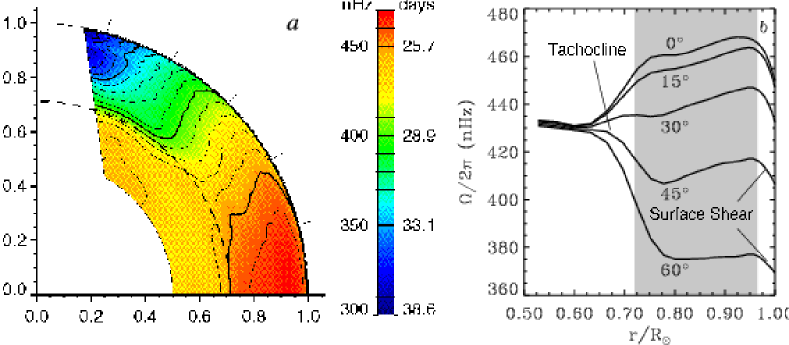
Figure 1.—  ($a$) Angular velocity profile $\Omega/2\pi$ with radius and latitude as deduced from helioseismology using SOI–MDI data, with red tones indicating fast rotation and blue-green the slowest rotation [adapted from Schou et al. 1998].  ($b$) Time-averaged rotation rates from five years of GONG helioseismic data, plotted against radius at different latitudes. The surface shear layer and the tachocline at the base of the convective zone are indicated, as well as the zone covered by our computational domain (grey area) [adapted from Howe et al. 2000b].

The tachocline has been one of the most surprising discoveries of helioseismology, especially since its strong rotational shear affords a promising site for the solar global dynamo. Such a tachocline was not anticipated, and current theoretical approaches to explain its presence are still only innovative sketches (Spiegel & Zahn 1992; Gough & McIntyre 1998; Charbonneau, Dikpati & Gilman 1999). Helioseismology has also recently detected prominent variations in the rotation rate near the base of the convective envelope, with a period of 1.3 years evident at low latitudes (Howe et al. 2000a; Toomre et al. 2000). These are the first indications of dynamical changes close to the presumed site of the global dynamo as the cycle advances. Such a succession of developments from helioseismology provide both a challenge and a stimulus to theoretical work on solar convection zone dynamics.

Seeking to understand solar differential rotation and magnetism requires 3–D simulations of convection in the correct full spherical geometry. However, the global nature of such solutions represent a major computational problem, given that the largest scale is pinned and only three orders of magnitude smaller in scale can be represented. Much of the small-scale dynamics in the sun dealing with supergranulation and granulation are by necessity then largely omitted. The alternative is to reduce the fixed maximum scale by studying smaller localized domains within the full shell and utilizing the three orders of magnitude to encompass the dynamical range of turbulent scales. There are clear tradeoffs:  the global models operate in the correct geometry yet struggle to encompass enough of a dynamical range to admit fully turbulent solutions, whereas the local models are able to study intensely turbulent convection but only within a particular limited portion of the full domain. Both approaches are needed, and the efforts are complementary, as reviewed in detail by Gilman (2000) and Miesch (2000). Highly turbulent but localized 3–D portions of a convecting spherical shells are being studied to assess transport properties and topologies of dynamical structures (e.g. Brandenburg et al. 1996; Brummell et al. 1996, 1998; Porter & Woodward 2000; Robinson & Chan 2001), of penetration into stable domains below (Brummell et al. 2001, Porter & Woodward 2001), of effects of realistic near-surface physics on granulation and supergranulation (e.g. Stein & Nordlund 1998), and of dynamo processes and magnetic transport by the convection (e.g. Cattaneo 1999, Tobias et al. 2001). Without recourse to direct simulations, the angular momentum and energy transport properties of turbulent convection have also been considered using mean-field approaches to derive second-order correlations (the Reynolds stresses and anisotropic heat transport) under the assumption of separability of scales. Although such procedures involve major uncertainties, the resulting angular momentum transport, which is described by mechanisms such as the so-called $\Lambda$ effect, have served to reproduce the solar meridional circulation (e.g. Durney 1999, 2000) and differential rotation (e.g. Kichatinov & Rüdiger 1995). Various other states can be achieved by adjusting parameters.

Initial studies of convection in full spherical shells to assess effects of rotation with correct account of geometry (e.g. Gilman & Miller 1981; Glatzmaier & Gilman 1982; Glatzmaier 1985, 1987; Sun & Schubert 1995) have set the stage for our efforts to study more turbulent flows using new numerical codes designed for the massively parallel computer architectures that are enabling such major simulations. We here report on our continuing studies with the anelastic spherical harmonic (ASH) code (Clune et al. 1999) to examine the $\Omega$ profiles established within the bulk of the solar convection zone by turbulent convection, building on the progenitor work by Miesch et al. (2000), Elliott, Miesch & Toomre (2000), and Brun & Toomre (2001). We also recognize the recent modelling of convection in spherical shells by Takehiro & Hayashi (1999) and Grote & Busse (2001).

The simulations reported in Miesch et al. (2000) and Elliott et al. (2000) have revealed the richness and complexity of compressible convection achieved in rotating spherical shells. Most of the resulting angular velocity profiles in the seven simulations considered have begun to make substantial contact with the helioseismic deductions within the bulk of the solar convection zone. These possess fast equatorial rotation (prograde), substantial $\Omega$ contrasts with latitude, and reduced tendencies for rotation to be constant on cylinders. The simulations with ASH have not yet sought to deal with questions of the near-surface rotational shear layer nor with the formation of a tachocline near the base of the convection zone. These studies have revealed that to achieve fast equators it is essential that parameter ranges be considered in which the convection senses strongly the effects of rotation, which translates into having a convective Rossby number less than unity for large Taylor numbers. Such rotationally-constrained convection exhibits downflowing plumes that are tilted away from the local radial direction, resulting in velocity correlations and thus Reynolds stresses that are found to have a significant role in the redistribution of angular momentum. This seems to provide paths to realize solar-like $\Omega$ profiles. Further, it is desirable to impose thermal boundary conditions at the top of the domain that enforce the constancy of emerging flux with latitude in order to be consistent with what appears to be observed.

We wish to focus on two outstanding issues raised by the prior simulations with ASH that need particular attention concerning the differential rotation established within the bulk of the solar convection zone. As Issue 1, the helioseismic inferences in Figure 1 emphasize that $\Omega$ in the sun appears to decrease significantly with latitude even at mid and high latitudes, a property which has been difficult to attain in the prior seven simulations. The substantial latitudinal decrease in angular velocity, say $\Delta\Omega$, in the models is primarily achieved in going from the equator to about 45^∘, with little further decrease in $\Omega$ achieved at higher latitudes in most of the cases. Whereas the overall latitudinal contrasts from equator to pole in the models and in the sun are roughly of the same order, the angular velocity in the sun continues to slow down much more as the pole is approached. Two models, designated as LAM (in Miesch et al. 2000) and L3 (in Elliott et al. 2000), do exhibit $\Omega$ which decrease at high latitudes, but LAM involves an emerging heat flux that varies too much with latitude due to choice of boundary conditions, and L3 has an overall $\Delta\Omega$ that is only two-thirds of the helioseismic value. Thus in confronting Issue 1, we will search in parameter space for solutions that can achieve $\Omega$ profiles in which the decrease with latitude does not taper off at mid latitudes and for which the contrast $\Delta\Omega$ is at least comparable to the helioseismic findings.

As Issue 2, with the convection becoming more turbulent, achieved by decreasing either the thermal or viscous diffusivities, there is a tendency for the latitudinal contrast $\Delta\Omega$ in the solutions to diminish or even decrease very prominently, thus being at variance with $\Delta\Omega$ deduced from helioseismology. This behavior appears to arise from increasing complexity leading to a weakening of nonlinear velocity correlations that have a crucial role in angular momentum redistribution. These Reynolds stress terms are strong in the laminar solutions that involve tilted columnar convection cells (‘banana cells’) aligned with the rotation axis; they weaken as the flows become more intricate, but would be expected to become again significant once coherent structures develop at higher levels of turbulence. For example, the model TUR (in Miesch et al. 2000) exhibits the emergence of downflow networks involving fairly persistent plumes which possess some of the expected attributes of the coherent structure seen in localized domains of highly turbulent convection (e.g. Brummell et al. 1998). As a result, TUR has a fairly interesting angular momentum transport attributed to the nonlinear correlations that sustain a level of differential rotation slightly weaker than LAM, but it too has a considerable variation of heat flux with latitude. The model T2 (in Elliott et al. 2000) sought to correct the latter by using modified thermal boundary conditions but appears to not have attained high enough turbulence levels to realize strong coherent structures. Absent those features, T2 yielded $\Omega$ profiles with a small $\Delta\Omega$, and even a slightly slower equatorial rotation rate than that in the mid latitudes. Thus in confronting Issue 2, we seek turbulent solutions that possess $\Omega$ profiles with fast equators and strong latitudinal contrasts $\Delta\Omega$, and emerging heat fluxes that vary little with latitude. To achieve this we have considered two paths in parameter space that yield more turbulent solutions by either varying the Prandtl number or keeping it fixed, while maintaining the same rotational constraint as measured by a convective Rossby number.

We describe briefly in §2 the ASH code and the set of parameters used for the simulations studied here. In §3 we discuss the properties of rotating turbulent convection and the resulting differential rotation and the meridional circulation for the five cases $A$, $AB$, $B$, $C$ and $D$. In §4 we analyze the transport of angular momentum by several processes and the influence of baroclinic effects in establishing the mean flows. In §5 we reflect on the significance of our findings, and especially in terms of dealing with the two issues raised by the prior simulations with ASH.

2. FORMULATING THE MODEL

Our numerical models are intended to be a faithful if highly simplified descriptions of the solar convection zone. In brief overview, solar values are taken for the heat flux, rotation rate, mass and radius, and a perfect gas is assumed since the upper boundary of the shell lies below the H and He ionization zones; contact is made with a real solar structure model for the radial stratification being considered. The computational domain extends from about 0.72$R_{\odot}$ to 0.96$R_{\odot}$, where $R_{\odot}$ is solar radius, with such shells having an overall density contrast in radius of about 25, and as a concequence compressibility effects are substantial. Thus we are concerned only with the central portion of the convection zone, dealing neither with the penetrative convection below that zone, nor the two shear layers present at the top and bottom of it. Given the computational resources available, we prefer to concentrate our effort on processes that establish the primary differential rotation in the bulk of the convection zone, and in future studies will seek to incorporate the other regions. We have as well softened the effects of the very steep entropy gradient close to the surface that would otherwise favor the driving of very small granular and mesogranular scales of convection, with these requiring a spatial resolution at least ten times greater than presently available.

The ASH code solves the 3–D anelastic equations of motion in a rotating spherical shell geometry using a pseudo-spectral semi-implicit approach (Clune et al. 1999). As discussed in detail in Miesch et al. (2000), these equations are fully nonlinear in velocity variables and linearized in thermodynamic variables with respect to a spherically symmetric mean state having a density $\bar{\rho}$, pressure $\bar{P}$, temperature $\bar{T}$ and specific entropy $\bar{S}$ and perturbations about this mean state of $\rho$, $P$, $T$, $S$. The conservation of mass, momentum and energy (or entropy) in a rotating reference frame are thus expressed as

$$\mbox{\boldmath$\nabla$}\cdot(\bar{\rho}{\bf v})=0,$$ (1)

$$\bar{\rho}\left(\frac{\partial{\bf v}}{\partial t}+({\bf v}\cdot\mbox{\boldmath$\nabla$}){\bf v}+2{\bf\Omega_{o}}\times{\bf v}\right)=-\mbox{\boldmath$\nabla$}P$$

$$+\rho{\bf g}-\mbox{\boldmath$\nabla$}\cdot\mbox{\boldmath$\cal D$}-[\mbox{\boldmath$\nabla$}\bar{P}-\bar{\rho}{\bf g}],$$ (2)

$$\bar{\rho}\bar{T}\frac{\partial S}{\partial t} = \mbox{\boldmath$\nabla$}\cdot[\kappa_{r}\bar{\rho}c_{p}\mbox{\boldmath$\nabla$}(\bar{T}+T)+\kappa\bar{\rho}\bar{T}\mbox{\boldmath$\nabla$}(\bar{S}+S)]$$

$$- \bar{\rho}\bar{T}{\bf v}\cdot\mbox{\boldmath$\nabla$}(\bar{S}+S)+2\bar{\rho}\nu\left[e_{ij}e_{ij}-1/3(\mbox{\boldmath$\nabla$}\cdot{\bf v})^{2}\right]$$

where $c_{p}$ is the specific heat at constant pressure, ${\bf v}=(v_{r},v_{\theta},v_{\phi})$ is the local velocity in spherical geometry in the rotating frame of constant angular velocity ${\bf\Omega_{o}}$, ${\bf g}$ the gravitational acceleration, $\kappa_{r}$ the radiative diffusivity, and ${\bf\cal D}$ the viscous stress tensor, with components

$${\cal D}_{ij}=-2\bar{\rho}\nu[e_{ij}-1/3(\mbox{\boldmath$\nabla$}\cdot{\bf v})\delta_{ij}],$$ (4)

where $e_{ij}$ is the strain rate tensor. Here $\nu$ and $\kappa$ are effective eddy diffusivities for vorticity and entropy. To close the set of equations, the linearized relations for the thermodynamic fluctuations are

$$\frac{\rho}{\bar{\rho}}=\frac{P}{\bar{P}}-\frac{T}{\bar{T}}=\frac{P}{\gamma\bar{P}}-\frac{S}{c_{p}},$$ (5)

assuming the ideal gas law

$$\bar{P}={\cal R}\bar{\rho}\bar{T},$$ (6)

where ${\cal R}$ is the gas constant. The bracketed term in equation (2), $\mbox{\boldmath$\nabla$}\bar{P}-\bar{\rho}{\bf g}$, vanishes initially because the mean state begins in hydrostatic balance from a one-dimensional radial solar model (Brun, Turck-Chièze & Zahn 1999), but as the convection becomes established this term becomes nonzero through effects of turbulent pressure. It is essential to take into account effects of compressibility upon the convection, since the solar convection zone spans many density scale heights. To accommodate this, we use the anelastic approximation (Gough 1969) to filter out the sound waves and therefore permit bigger time steps for the temporal evolution. The latter is allowed since the CFL (Courant, Friedrichs & Lewy) numerical stability condition now applies to the smaller convective velocities rather than the sound speed $c_{s}$.

Due to the small solar molecular viscosity, direct numerical simulations (DNS) of the full scale range of motions present in stellar convection zones are currently not feasible. We seek to resolve the largest scales of convective motion that we believe are the main drivers of the solar differential rotation, doing so within a large-eddy simulation (LES) formulation where $\nu$ and $\kappa$ are assumed to be an effective eddy viscosity and eddy diffusivity that represent unresolved subgrid-scale (SGS) processes, chosen to suitably truncate the nonlinear energy cascade. For simplicity, both are here taken to be functions of radius alone, and are chosen to scale as the inverse of mean density. Other forms that may be determined from the properties of the large-scale flows according to one of many prescriptions (e.g. Lesieur 1997, Canuto 1999) will be considered in the future. We have also introduced an unresolved enthalpy flux proportional to the mean entropy gradient in equation (3) in order to account for transport by small-scale convective structures near the top of our domain (Miesch et al. 2000). We utilize the same radial profile for that mean eddy diffusivity in our five cases in order to minimize the impact of our SGS treatment on the main properties of our solutions. We emphasize that currently tractable simulations are still many decades away in parameter space from the intensely turbulent conditions encountered in the sun, and thus these large-eddy simulations must be viewed as training tools for developing our dynamical intuition of what might be proceeding within the solar convection zone.

Within the ASH code, the mass flux is imposed to be divergence-free by using poloidal $W$ and toroidal $Z$ functions. The thermodynamic variables $P$ and $S$, and $W$ and $Z$, are expanded in spherical harmonics $Y^{m}_{\ell}(\theta,\phi)$ to resolve their horizontal structures and in Chebyshev polynomials $T_{n}(r)$ to resolve their radial structures. This approach has the distinct advantage that the spatial resolution is uniform everywhere on a sphere when a complete set of spherical harmonics is used in degree $\ell$ (retaining all azimuthal orders $m$). We expand up to degree $\ell=\ell_{max}$ (depending on the number of latitudinal mesh points $N_{\theta}$, e.g. $\ell_{max}=(2N_{\theta}-1)/3$), utilize as longitudinal mesh points $N_{\phi}=2N_{\theta}$, and employ $N_{r}$ collocation points in projecting upon the Chebyshev polynomials. In this study the highest resolution used has $\ell_{max}=340$ and $N_{r}=193$. The time evolution is carried out using an implicit, second-order Crank-Nicholson scheme for the linear terms and an explicit, second-order Adams-Bashforth scheme for the advective and Coriolis terms.

Within ASH, all spectral transformations are applied to data local to each processor, with inter-processor transposes performed when necessary to arrange for the transformation dimension to be local. The triangular truncation in spectral space precludes any simple distribution of the data and workload among the nodes. For very large problems, the Legendre transformations dominate the workload and, as a result, great care has been taken to optimize their performance on cache-based architectures. Arrays and loops have been structured to operate on blocks which minimize cache misses. The ASH code is extremely flexible and has demonstrated excellent scalability on massively parallel supercomputers such as the Cray T3E, IBM SP-3 and Origin 2000.

As boundary conditions, we impose impenetrable and stress-free conditions for the velocity field and constant flux (i.e constant entropy gradient) both at the inner and outer boundaries. We seek solutions with an emerging flux at the top that is invariant with latitude (Issue 2). As initial conditions, we have started some simulations (cases $A$, $B$) from quiescent conditions of uniform rotation, and others (cases $AB$, $C$, $D$) from evolved solutions in which we modify certain diffusivities. This leads to changes in the effective Rayleigh number $R_{a}$, the Prandtl number $P_{r}$, the Péclet number $P_{e}$, the Reynolds number $R_{e}$ and the Taylor number $T_{a}$, while keeping constant the convective Rossby number $R_{oc}$, all of which are defined in Table 1. We also summarize there the parameters of the five simulation cases.

3. PROPERTIES OF TURBULENT COMPRESSIBLE CONVECTION

We have conducted five simulations involving increasingly nonlinear flows that are achieved by reducing the viscous and entropy diffusivities in the manner outlined in Table 1. We have followed two paths in parameter space in obtaining more complex convective flows. On Path 1 in going from case $A$ to $C$ via $B$, we incrementally decreased the eddy viscosity $\nu$ while keeping the eddy diffusivity $\kappa$ constant, thereby reducing the Prandtl number $P_{r}$ by a factor 8. In particular, the laminar case $A$ has $P_{r}$ of unity; reducing the viscosity by a factor of 4 leads to the mildly turbulent case $B$ with $P_{r}=0.25$, or by a factor of 8 leads to the more turbulent case $C$ with $P_{r}=0.125$. This serves to increase the Reynolds number $R_{e}$ while only mildly increasing the Péclet number $P_{e}$. Path 2 kept the Prandtl number fixed at $P_{r}=0.25$ as the complexity of the flows was increased by reducing both diffusivities. Starting from case $AB$, we go to case $B$ by decreasing both diffusivities $\nu$ and $\kappa$ by a factor of 2, and then to our most turbulent case $D$ by further reducing both by a factor of 2 relative to case $B$. This Path 2 in going from case $AB$ to $D$ via $B$ results in both $R_{e}$ and $P_{e}$ increasing comparably. All our models possess a convective Rossby number $R_{oc}$ of order 2/3, thus maintaining a strong rotational constraint on the convection.

As we shall describe in some detail, the resulting vigorous convection influenced by rotation in all these cases is intricate and richly time dependent, much as found in Miesch et al. (2000) and Elliott et al. (2000). It is characterized by networks of strong downflow at the periphery of the convection cells, and weaker upflows in their middle, both of which are a consequence of the effects of compressibility as we consider flows that can span multiple density scale heights in the vertical. Indeed, we consistently observe that the downflows are able to extend over the full depth of the unstable layer, appearing as twisted sheets of downflow near the top and more distinctive plumes deeper in the layer. These downflow networks essentially represent coherent structures amidst the turbulence, and they are found to have a most significant role in the nonlinear transport of angular momentum by yielding correlations between different velocity components that form Reynolds stress terms. We find that the convection in all cases studied here is able to redistribute angular momentum in such a manner that substantial differential rotation profiles are established, the properties of which are the major focus of this work.

3.1. Complex evolution of convective patterns

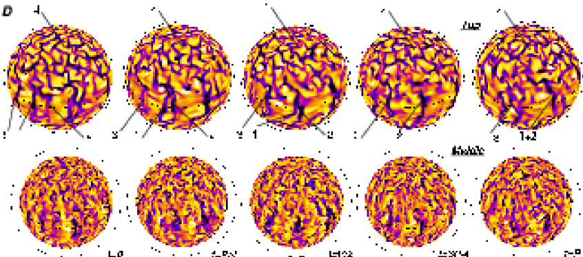
Figure 2.— Evolution of the convection throughout one solar rotation, showing the radial velocity of case $D$ near the top and at the middle of the domain. The time interval between each successive image is about 7 days. Features 1 and 2 exhibit the merging of the downflow lanes, feature 3 the shearing action of the differential rotation present in the shell and feature 4 the appearance and deformation of a convective cell at higher latitudes.

The time dependence in our most turbulent simulation (case $D$) is shown in Figure 2 which displays two sequence of images of the radial velocity on spherical surfaces over the course of one full rotation. The upper sequence with views near the top of the layer involves simpler downflow networks (shown in darker tones) that are easier to intercompare from frame to frame, whereas the lower ones with views in the middle of the convecting layer are more difficult to track because of increased complexity of the patterns in the more turbulent flows there. The vantage point is in the uniformly rotating frame used in our modelling, and some of the pattern evolution results from the prograde zonal flows at low latitudes and retrograde ones at high latitudes associated with the differential rotation relative to this frame. There is further melding and shearing of particular downflow lanes as the convection cells evolve over a broad range of time scales, some of which are comparable to the rotation period. This is particularly evident in some of the downflow structures identified near the equatorial region in the upper sequence, with features labeled 1 and 2 illustrating the merging of two downflow lanes, and feature 3 the typical distortion of a lane which also involves both a site of cyclonic swirl in the northern hemisphere and another that is appropriately anticyclonic in the southern hemisphere. The behavior at higher latitudes that involves retrograde displacement of the downflow networks is somewhat more intricate, partly because the convection cells are of smaller scale and exhibit the frequent formation of new downflow lanes (as in feature 4) that can serve to cleave existing cells. Figure 2 emphasizes that the overall pattern of these global cells is sufficiently modified during the course of one rotation period so that it would be difficult to identify particular structures (relative to our uniformly rotating vantage point) when viewed in a subsequent rotation. This would suggest that giant cells possibly present within the solar convection zone may also loose their identity from one Carrington rotation to the next. This comes about both because of advection and distortion of the cells by the mean zonal flows associated with the differential rotation (here at the equator leading to relative angular displacements in longitude of about 70^∘ over one rotation period), and because of fairly rapid evolution and some propagation in their individual downflow patterns.

3.2. Downflow networks and variation with depth

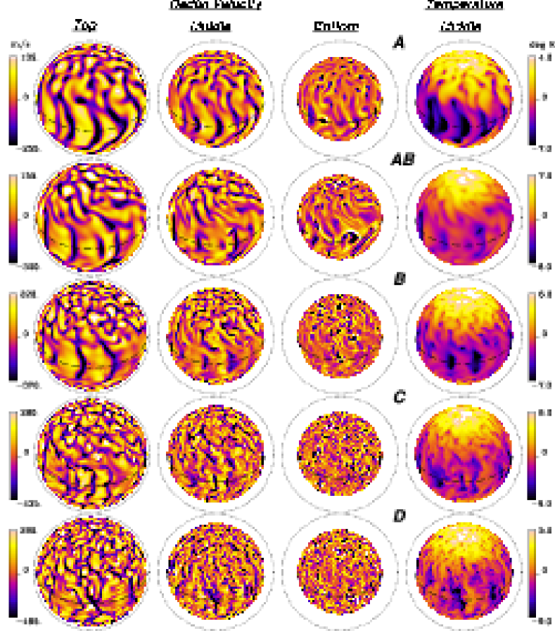
Figure 3.— Convective patterns for the five cases $A$, $AB$, $B$, $C$ and $D$ as increasingly turbulent flows are attained. The radial velocity shapshots are shown at three different depths (0.95, 0.84, 0.73 $R_{\odot}$). Downflows are represented in purple-dark tones and upflows in orange-bright tones, with dynamic ranges indicated. The dotted circle is positioned at radius R_⊙, and the equator is indicated by the dashed curve. The convective structures become more complex in this progression of cases, with the banana-like convective cells giving way to stronger and more frequent vortex sites. The strongest downflow lanes extend over the full depth range. The fluctuating temperature fields at mid depth are shown on the right, emphasizing that downflows are relatively cool and that the polar regions are on average warm.

The convective structures as delineated by the downflow networks show distinctive changes as the level of turbulence is increased in going from case $A$ to case $D$. Figure 3 provides an overview of radial velocity snapshots in our five simulations at three depths (near the top, middle and bottom), accompanied by the fluctuating temperature fields at mid-depth. The upper surface in all our cases involves a connected network of downflows surrounding broad upflows, but such smoothness can disguise far more turbulent flows below. The seemingly cellular motions near the surface result from the expansion of fluid elements rising through the rapidly decreasing density stratification near the upper boundary, aided also by our increasing viscous and thermal diffusivities there. As viewed near the top, the tendency of the convection in our laminar case $A$ to be organized into ‘banana cells’ nearly aligned with the rotation axis at low latitudes is progressively disrupted by increasing the level of complexity in going in turn to cases $AB$, $B$, $C$ and $D$. There is still some semblance of north-south alignment in the downflows even in our most turbulent case $D$, but the latitudinal span of this alignment is confined to a narrow interval around the equator. Clearly the downflow lanes become more wiggly and exhibit more pronounced vortical features and curvature in this sequence of cases. As well, the downflow networks involve more frequent branching points and smaller horizontal scales for the convective patterns, especially at higher latitudes. Given the three simultaneous views of the radial velocity, one can clearly identify downflow lanes near the top in all our cases that turn into distinctive plumes at greater depths, showing that organized flows extend over multiple scale heights. Indeed, the strongest downflows occur at the interstices of the upper network and are able to pierce through the interior turbulence, thus spanning the full depth range of the domain.

The plumes in the more turbulent cases $C$ and $D$ represent coherent structures that are embedded within less ordered flows that surround them. They are able to maintain their identity, though with some distortion and mobility, over significant intervals of time. Although these downflowing plumes are primarily directed radially inward, they show some tilt both toward the rotation axis and out of the meridional plane. This yields correlated velocity components and thus Reynolds stresses that are a key ingredient in the redistribution of angular momentum within the shell. Such tilting away from the local radial direction in coherent downflows has been seen in high-resolution local $f$-plane simulations of rotating compressible convection (Brummell et al. 1998), and their presence has a dominant role in establishing the mean zonal and meridional flows. We also refer to Rieutord & Zahn (1995) and Zahn (2000) for an analytical study of the transport properties and correlations present in such strong vortex structures and on their potential dynamical role in the solar convection zone.

The strong downflows shown in Figure 3 accentuate the asymmetries that are characteristic of compressible convection, with typical peak amplitudes in these downflows at mid-layer being as much as twofold greater than that in the upflows. As might be expected, the overall rms radial velocities listed in Table 2 increase with complexity in the flow fields in going from case $A$ to $D$. The asymmetries between upflows and downflows have the consequence that the kinetic energy flux in such compressible convection is directed radially inward, in contrast to the enthalpy and radiative fluxes that are directed outward in transporting the solar flux (see Figure 3.5$a$).

That enthalpy flux involves correlations between radial velocities and temperature fluctuations, and these are evidently strong as seen when inspecting the temperature and velocity fields shown at mid layer in Figure 3. Buoyancy driving within our thermal convection involves downflows that are cooler and thus denser and upflows that are warmer and lighter than the mean; there are systematic asymmetries in those temperature fluctuations, much as in the radial velocities. Further, in comparing the temperature maps with those of radial velocity in the middle of the layer, some of the temperature patterns are evidently smoother, which is a consequence of the greater thermal diffusivities than viscosities for cases with Prandtl numbers less than unity. A striking property shared by all these temperature fields is that the polar regions are consistently warmer than the lower latitudes, a feature that we will find to be consistent with a fast or prograde equatorial rotation.

3.3. Driving strong differential rotation

The differential rotation profiles with radius and latitude that result from the angular momentum redistribution by the vigorous convection in our five simulations are presented in Figure 4. In order to simplify comparison of our results with deductions drawn from helioseismology (Fig.1), we have converted our mean longitudinal velocities $\hat{v}_{\phi}$ (with $\hat{}$ denoting averaging in longitude and time) into a sidereal angular velocity $\Omega$ with radius and latitude, and note that our reference frame rotation rate $\Omega_{o}/2\pi$ is 414 nHz (or a period of 28 days). The angular velocity in all our cases exhibits substantial variations in time, and thus long time averages must be formed to deduce the time mean profiles of $\Omega$ shown in Figure 4. The layout of the five cases in Figure 4 reflects the two paths we have taken in increasing the complexity or turbulence level in the solutions: Path 1 in going from $A$ to $C$ via $B$ while decreasing the Prandtl number takes us from upper left to lower right, and Path 2 in going from case $AB$ to $D$ via $B$ while keeping the Prandtl number fixed at $P_{r}$=1/4 takes us from upper right to lower left. Complexity in the convective flows increases in going down the page.

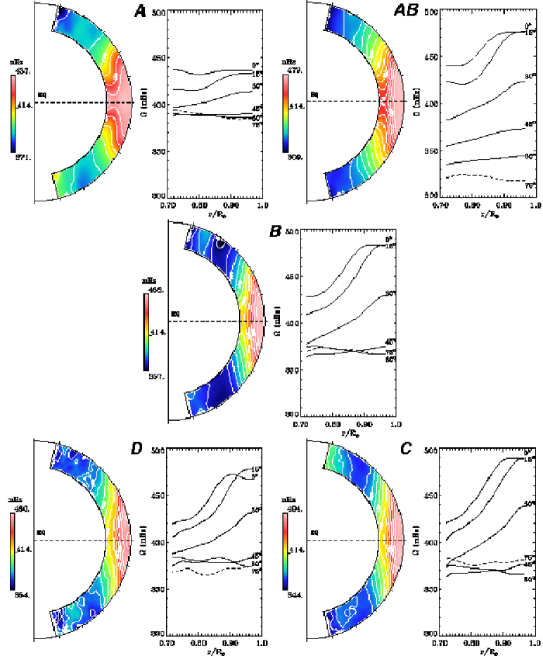
Figure 4.— Temporal and longitudinal averages of the angular velocity profiles achieved in cases $A$, $AB$, $B$, $C$ and $D$, formed over intervals in turn of 295, 275, 275, 175 and 35 days. The contour plots for $\Omega/2\pi$ on the left of each panel are independently scaled, whereas the radial cuts at the indicated latitudes share the same scaling to accentuate the overall behavior of the five cases. The crossed layout of the five cases emphasizes the two different paths followed to reach more turbulent states, mainly by lowering $P_{r}$ on Path 1 ($A\rightarrow B\rightarrow C$), and by lowering diffusivities while keeping $P_{r}$ constant on Path 2 ($AB\rightarrow B\rightarrow D$). All cases exhibit a prograde equatorial rotation and a strong contrast $\Delta\Omega$ from equator to pole. Case $AB$ possesses a high latitude region of particularly slow rotation.

All five simulations yield angular velocity $\Omega$ profiles that involve fast (prograde) equatorial regions and slow (retrograde) high latitude regions. The variation of $\Omega$ with radius and latitude may be best judged in the color contour plots in Figure 4 which are scaled independently for each of the cases; the reference frame rate is also indicated. The immediate polar regions are omitted in these plots because it is difficult to obtain stable mean $\Omega$ values at very high latitudes since the averaging domain there becomes very small whereas the temporal fluctuations in the flows remain substantial. The contour plots reveal that there are some differences in the $\Omega$ realized in the northern and southern hemispheres, though such symmetry breaking is modest and probably will diminish with longer averaging. The convection itself is not symmetric about the equator, and thus the mean zonal flows that accompany such convection, and which are manifest as differential rotation, can be expected to have variations in the two hemispheres. In cases $B$, $C$ and $D$, there is some alignment of the $\Omega$ contours at the lower latitudes with the rotation axis, thus showing a tendency for $\Omega$ to be somewhat constant on cylinders. Further, in these cases almost all the decrease in $\Omega$ with latitude occurs in going from the equator to about $45^{\circ}$, or thus is confined to the region outside the tangent cylinder to the inner boundary (which intersects the outer boundary in our shell configuration at $42^{\circ}$). In contrast, cases $A$ and $AB$ show far less alignment of $\Omega$ contours with cylinders at the lower latitudes, and at mid-latitudes the contours are nearly aligned with radial lines, more in the spirit of the helioseismic inferences.

Case $AB$ in Figure 4 is unique in having the monotonic decrease of $\Omega$ with latitude continue onward to high latitudes, which is also the trend deduced from helioseismic measurements. Thus Issue 1 concerned with achieving a consistently decreasing $\Omega$ at high latitudes is resolved with case $AB$. This is significant in showing that such behavior can be realized in our modelling of convection in deep shells, though it is not a common property in our other cases. It would be most desirable to understand how such high-latitude variation in $\Omega$ is achieved in case $AB$, and we will address this in §4.

The accompanying radial cuts of $\Omega$ at six fixed latitudes in Figure 4 permit us to readily quantify the $\Omega$ contrasts with latitude achieved in these solutions, and to judge the functional variation with radius in each case. We use a common scaling for all these line plots to make intercomparison between the cases most convenient; the radial cuts for $\Omega$ have been averaged between the north and south hemispheres. Near the top of the convection zone at radius 0.96$R$, the laminar convection in case $A$ produces a differential rotation with a contrast in angular velocity, or $\Delta\Omega/2\pi$, of about 50 nHz between the equator and 60^∘, or 12% relative to the frame rotation rate (also quoted in Table 2). Continuing on Path 1 in parameter space to the more turbulent cases $B$ and $C$, we find that the latitudinal contrast in angular velocity has increased substantially, becoming 115 nHz and 125 nHz in the two cases. These correspond in turn to a 28% and a 30% variation of the rotation rate. These values are of interest since the helioseismic inferences (Thompson et al. 1996, Schou et al. 1998, Howe et al. 2000b) have a contrast of about 92 nHz at a similar depth between the equator and 60^∘, or a variation of about 22% in rotation rate, which further increases to about 32% in going to 75^∘. The pronounced differential rotation in cases $B$ and $C$ is accompanied by the $\Omega$ profiles becoming somewhat more aligned with the rotation axis, resulting in steeper slopes in the radial cuts at low and mid latitudes. These two turbulent cases achieve their larger $\Delta\Omega$ by both faster equatorial rotation rates and slower rates at higher latitudes. Thus Path 1 has been able to resolve Issue 2, concerned with retaining a strong contrast $\Delta\Omega$ and a fast equator, as the solution becomes more complex and turbulent.

Turning to Path 2 in parameter space, case $AB$ shows a contrast of about 135 nHz between the equator and 60^∘, or a 33% variation of rotation rate, which further increases to about 160 nHz or 39% in going to 75^∘. The pivotal case $B$ has a somewhat reduced contrast $\Delta\Omega/2\pi$ of 115 nHz or 28% variation between equator and 60^∘, with little further variation at higher latitudes. The most turbulent case $D$ has a $\Delta\Omega/2\pi$ of about 105 nHz or a 25% variation between the equator and 60^∘. Thus Path 2 leads to a slight reduction in $\Delta\Omega$ with increasing complexity, unlike the behavior of Path 1. However, even this path yields a turbulent solution case $D$ whose $\Delta\Omega$ is still close to the helioseismic contrast, thus largely resolving Issue 2. This is reemphasized in Figure 3.3 which summarizes the variation of $\Delta\Omega$ with $P_{r}$ for our five cases.

Parameter space diagram for relative latitudinal angular velocity contrast $\Delta\Omega/\Omega_{o}$ as a function of the Prandtl number $P_{r}$ for the five cases. The two paths toward higher levels of turbulence either reduce $P_{r}$ ($A\rightarrow B\rightarrow C$), or maintain a constant $P_{r}$ ($AB\rightarrow B\rightarrow D$).

Most of our cases possess overall latitudinal contrasts in $\Omega$ that are in the realm of solar values deduced from inversion of helioseismic data, yet case $AB$ stands out in having the systematic decrease of $\Omega$ with latitude extending almost to the poles, which appears to be another distinguishing feature of the actual solar $\Omega$ profiles. Further, case $AB$ displays little radial variation in $\Omega$ at intermediate and high latitudes (from say 45^∘ onward) as the angular velocity continues to decrease poleward. Such behavior is most interesting, and it is necessary to understand just which convective properties within case $AB$ allow it to come into reasonable contact with the helioseismic profiles for $\Omega$ deduced in the bulk of the solar convection zone.

The $\Omega$ profiles in Figure 4 have been formed from temporal averages spanning multiple rotation periods as indicated. It is appropriate to consider if these represent truly ‘spun-up’ solutions in a statistical sense, and further whether several distinctive $\Omega$ profiles could be achieved for the same control parameters. Both issues may be intertwined, for the rate of approach to equilibration can be influenced by the attraction characteristics of that differential rotation state, and of course by the amplitude of the fluxes available to redistribute angular momentum to achieve that state (see §4.1). This overall dynamical system of turbulent convection is sufficiently complex that we are uncertain whether there may exist multiple basins of attraction leading to different classes of differential rotation. For instance, is the behavior of case $AB$ with noticeably slow rotation at high latitudes an example of one class of behavior, and our other cases that of another family? Could such families overlap in parameter space, or are there just gradual variations in behavior in $\Omega$ with changes in the parameters? We have so far sought to address some of these questions by perturbing the evolving solutions to see if they might flip to another state, but they have not done so. We plan to examine such issues of solution uniqueness in our follow on studies in which we seek to extend the slow-pole characteristics of case $AB$ to other parameter settings involving more complex convection.

As to the relative maturity of the spun-up states shown in Figure 4, these vary from case to case due to the rapidly increasing computational expense in dealing with the finer spatial resolution required by the more complex simulations. Cases $AB$ and $C$ were both started from case $B$ that had already been run for over 4000 days of elapsed simulation time (or a nominal 143 rotation periods involving about 28 days each). At this point case $B$ appeared to be statistically stationary in terms of the kinetic energy associated with the differential rotation, though it like most of the other simulations exhibit small fluctuations in $\Omega$ profiles determined from single-rotation averages, especially at the higher latitudes. Case $AB$ was evolved for about 2300 days (82 rotation periods), and we illustrate in Figure 3.3$a$ a succession of $\Omega$ profiles with latitude sampling the last 600 days in the simulation. The solid curve there is an average formed over 10 rotations (consistent with the contour plot in Figure 4), and we see that the individual rotation averages being sampled form a narrow envelope around it. There is evidently some symmetry breaking between the two hemispheres. We believe that the differential rotation for case $AB$ is now an effectively stationary state (as is also confirmed in studying the angular momentum flux balance in Figure 6). The more turbulent case $C$ was evolved for about 500 days (18 rotations) after being initiated from case $B$, and a set of its angular velocity profiles are shown sampling the last 300 days in Figure 3.3$b$. We are less certain of its stationarity, but we could not detect any systematic trends in the evolution of its differential rotation over the last 10 rotations. We saw no evidence of a slow pole developing, but that may well require more extended computations than could be presently arranged. Figure 3.3 serves to emphasize that the angular velocity even in the sun may be expected to vary somewhat from one rotation to another, with the samplings here providing a sense of the amplitude of those changes.

Succession of time-averaged $\Omega$ profiles with latitude at $r=0.96R_{\odot}$.  $(a)$ For case $AB$, a numbered sequence of single-rotation averages spanning an interval of 600 days in the late evolution of the system, with the bold curve 4 denoting an average over the last 275 days in the simulation.  $(b)$ For case $C$, dealing with samples in a 300 day interval, and the bold curve 4 representing an average over the final 175 days. The variations are representative of small changes in the differential rotation that accompany changes in the convection once a mature statistical state has been achieved.

Figure 5.— Temporal and longitudinal averages of the meridional flows achieved in the cases $A$, $AB$, $B$, $C$ and $D$, deduced from sampling in turn 295, 275, 275, 175 and 35 days. Shown are random streaklines whose length is proportional to flow speed, with arrowheads indicating flow sense. The typical speeds in these meridional circulations are about 20 m s^-1. For all the cases strong poleward cells are present near the surface at low latitudes as well as return flows at mid depth.

3.4. Meridional circulation patterns

The time-averaged meridional circulations that accompany the vigorous convection in the five cases are shown in Figure 5. The typical amplitudes in these large-scale circulations are about 20 m s^-1, and thus comparable to the values deduced from local domain helioseismic probing of the uppermost convection zone based either on time-distance methods (e.g. Giles, Duvall & Scherrer 1998) or ring-diagram analyses (Schou & Bogart 1998, Haber et al. 1998). There is little change in meridional circulation amplitudes as we increase the level of turbulence in going from case $A$ to $D$. However, multi-cell structures in these circulations become more intricate with the increased complexity of the convection. At lower latitudes the circulation in both hemispheres is poleward near the top of the domain, with return flows at various depths. All cases display multiple cells with radius and latitude, and never only one big meridional cell as often used in mean field models dealing with differential rotation (e.g. Rekowski & Rüdiger 1998, Durney 2000) or with Babcock-Leighton dynamos (e.g. Choudhuri, Schüssler & Dikpati 1995, Dikpati & Charbonneau 1999). The resulting axisymmetric meridional circulation is maintained by Coriolis forces acting on the mean zonal flows that appear as the differential rotation, by buoyancy forces, by Reynolds stresses, and by pressure gradients. Given these competing processes, it is not self evident as to what pattern of circulation cells should result, nor how many should be present in depth or latitude. Our five simulations have shown that there is some variety in the meridional circulations achieved, all of which involve multi-celled structures. Since the kinetic energy in the meridional circulation (MCKE) is typically about two orders of magnitude smaller than in the differential rotation (DRKE), as we will detail in §3.5 and in Table $2$, small variations in the differential rotation can yield substantial changes in the circulations. This is likewise true of the time-varying Reynolds stresses from the evolving convection which again has a kinetic energy (CKE) much larger than that of the meridional circulations. This may explain the complex time dependence realized by the meridional flows, and the need to use long time averages in defining their mean properties.

Another rendition of the time-averaged meridional circulations achieved in cases $AB$ and $C$ is shown in Figure 3.4 using a streamfunction $\Psi$ based on the zonally-averaged mass flux [as in Miesch et al. 2000, equation (7)]. In case $AB$ (Fig. 3.4$a$) there are two circulation cells positioned above each other in radius at low latitudes. The stronger upper one (solid contours representing counterclockwise circulation) involves poleward flow that extends from the equator to about 30^∘ latitude near the top of the domain in the northern hemisphere. The southern hemisphere has likewise poleward flow near the top at low latitudes, with ascending motions again present from the equator to about 20^∘ latitude. At latitudes greater than about 30^∘ the relatively weak flow near the top is mainly equatorward in both hemispheres, but exhibits fluctuations.

A quantitative measure of this for case $AB$ is provided in Figure 3.4$a$ that displays the mean velocity component $\hat{v}_{\theta}$ with latitude at two depths near the top of the domain. The poleward flow in both hemispheres peaks at about 20^∘ latitude and then decreases rapidly, changing to weak equatorward flow above 30^∘ which attains about one-third that peak amplitude.

Streamlines of the mean axisymmetric meridional circulation achieved in $(a)$ case $AB$ averaged over 275 days, and in $(b)$ case $C$ averaged over 175 days. Solid contours denote counterclockwise circulation (and dashed clockwise), equally spaced in value. In case $AB$, two circulation cells are present with radius at low latitudes, and only weak circulations at latitudes above 30^∘. Case $C$ possesses three cells at low latitudes, with the deepest extending prominently to high latitudes.

Turning to case $C$ in Figure 3.4$b$, it exhibits three circulation cells positioned radially at low latitudes, with the outermost again yielding poleward flow at the top of the domain that extends to about 35^∘ in latitude. At higher latitudes the mean meridional flow is again equatorward near the top, attaining a peak amplitude for $\hat{v}_{\theta}$ (detailed in Figure 3.4$b$) that is comparable to the poleward one from the low latitudes, unlike in case $AB$. Of the three meridional cells at low latitudes in Case $C$, much as for model TUR in Miesch et al. 2000 (cf. Fig. $16a$), the deepest cell involves a strong counterclockwise circulation that extends to high latitudes, yielding a submerged poleward flow there that lies below the equatorward flow at the top of the domain. Such behavior involving a third deep circulation cell that extends to high latitudes is also seen in cases $B$ and $D$. Such a strong third cell appears to be of significance in the continuing net poleward transport of angular momentum by the meridional circulations (cf. §4.1, Fig. 6) in all these cases at latitudes above about 30^∘. This is not realized in case $AB$, and may contribute to its slow pole behavior. It is encouraging that we have poleward circulations in the upper regions of the simulations, which is in accord with the general sense of the mean flows near the surface being deduced from local helioseismology, though two cell behavior with latitude has been detected recently only in the northern hemisphere near the peak of solar activity (Haber et al. 2000). Such symmetry breaking in the two solar hemispheres is an interesting property, and one that is also occasionally realized in our simulations as the convection patterns evolve. The helioseismic probing with ring diagram methods and explicit inversions is able to sense the meridional circulations only fairly close to the solar surface, typically extending to depths of about 20 Mm or to radius 0.97 $R_{\odot}$, whereas our simulations have their upper boundary slightly below this level at 0.96 $R_{\odot}$.

Mean velocity component $\hat{v}_{\theta}$ with latitude at the two depths $r=0.96R_{\odot}$ (solid) and $0.94R_{\odot}$ (dash dot), showing in $(a)$ case $AB$ and in $(b)$ case $C$. Positive values correspond to flow directed from north (positive latitudes) to south (negative latitudes). At low latitudes the flows are poleward in both hemispheres, but whereas case $C$ exhibits fairly strong equatorward flow at latitudes above 35^∘, case $AB$ possesses much weaker circulations there.

Thus we must be cautious in interpreting similar behavior in the meridional circulations since our models and the ring diagram analysis do not explicitly overlap in radius. Helioseismic assessments based on time-distance methods (Giles 1999, Chou & Dai 2001) and annular rings centered on the poles (Braun & Fan 1998) report detecting effects attributable to meridional circulations with a mainly poleward sense to depths corresponding to 0.90 $R_{\odot}$ or even 0.85 $R_{\odot}$. Such results are most interesting, but considerable further work on inversions would be required to provide detailed profiles of the circulations with depth. As these mappings become available, they may be able to confirm or refute the multi-cell radial structure of meridional circulation (Fig. 5) typically realized in our simulations.

3.5. Energetics of the convection and the mean flows

The overall energetics within these shells of rotating convection have some interesting properties, in addition to the mean zonal and meridional flows that coexist with the complex convective motions. The convection is responsible for transporting outward the solar flux emerging from the deep interior. We should recall, as discussed in detail in Miesch et al. (2000), that the radial flux balance in these convective shells involves four dominant contributors, namely the enthalpy or convective flux $F_{e}$, the radiative flux $F_{r}$, the kinetic energy flux $F_{k}$, and finally the unresolved eddy flux $F_{u}$, which add up to form the total flux $F_{t}$. Figure 3.5$a$ shows the flux balance with radius achieved in our most turbulent case $D$ as averaged over horizontal surfaces and converted to luminosities. The radiative flux becomes significant deep in the layer due to the steady increase of radiative conductivity with depth, and indeed by construction it suffices to carry all the imposed flux through the lower boundary of our domain where the radial velocities and thus the convective flux vanishes. A similar role near the top of the layer is played by the sub-grid-scale turbulence that yields $F_{u}$, which being proportional to a specified eddy diffusivity function $\kappa$ and the mean radial gradient of entropy, suffices to carry the total flux through the upper boundary and prevents the entropy gradient there from becoming too superadiabatic compared to the scales of convection that we are prepared to resolve spatially. Over most of the interior of the shell, the strong correlations between radial velocities and temperature fluctuations yield the enthalpy flux $F_{e}$ that transports upward almost all of the imposed flux, and this peaks near the middle of the layer. The kinetic energy flux $F_{k}$ works against the others by being directed downward, a result of the fast downflow sheets and plumes achieved by effects of compressibility (Hurlburt, Toomre & Massaguer 1986). These general properties are shared by our five cases, all of which have achieved good overall flux balance with radius, as can be assessed by examining $F_{t}$.

Figure 3.5$b$ presents the kinetic energy spectra with azimuthal wavenumber $m$ at three depths, and averaged in time, as realized in the case $D$ simulation. The spectra are fairly broad, with a plateau of power extending up to about $m$=30 corresponding to some of the most vigorously driven scales, and then a rapid decrease involving about 5 orders of magnitude to the highest wavenumber of 340. The decrease is more rapid for the spectra formed near the top of the shell. These spectra suggest that the flows are well resolved, with a reasonable scale separation between the dominant energy input range and the wide interval over which dissipation functions. We cannot readily identify a clear inertial subrange, though for reference we include some power laws. We also refer to Hathaway et al. (1996, 2000) for a discussion of recent observational inferences about the solar kinetic energy spectrum which does not seem to indicate any clear scaling law.

($a$) Radial transport of energy in case $D$ achieved by the fluxes $F_{r}$, $F_{e}$, $F_{k}$ and $F_{u}$, and their total $F_{t}$, all normalized by the solar luminosity. ($b$) Time averaged azimuthal wavenumber spectra of the kinetic energy on different radial surfaces (solid curve $r/R_{\odot}$=0.95; dashed, 0.84; dotted, 0.73) for case $D$ with $l_{max}=340$. The results have been averaged over 35 days. Superimposed are the power laws $k^{-5/3}$, $k^{-2}$ and $k^{-3}$; no clear inertial subrange is identifiable.

Table 2 summarizes various rms velocities that characterize our five simulations as sampled in the middle of the layer where the enthapy flux also peaks. The rms radial velocity $\tilde{v}_{r}$ increases monotonically in going through the sequence of cases $A$, $AB$, $B$, $C$ to $D$. The associated rms Reynolds number $\tilde{R}_{e}$ in Table 1 increases also (though part of this is due to changes in the diffusivities), varying by a factor of about 15 from our laminar to most turbulent solutions. The rms longitudinal velocity $\tilde{v}_{\phi}$ has the greatest amplitude in all the cases. However a removal of the mean zonal flow component responsible for the differential rotation yields $\tilde{v}_{\phi}^{\prime}$. Comparison of this with the radial and latitudinal rms velocities reveals that all possess very comparable amplitudes, suggesting fairly isotropic convective motions near the midplane. Table 2 also assesses the volume and time averaged total kinetic energy (KE), that associated with the differential rotation (DRKE), with the meridional circulation (MCKE), and with the convection itself (CKE). In all of our solutions the DRKE and CKE are comparable, and the MCKE is much smaller. Table 2 reveals a most interesting contrast in behavior for the two paths. Following Path 1 (involving $A$, $B$ and $C$, with decreasing $P_{r}$), we find that KE in the solutions increases steadily with increasing flow complexity. This would be expected since the buoyancy driving has strengthened relative to the dissipative mechanisms as measured by the increasing Rayleigh number $R_{a}$ (Table 1). Path 2 (involving $AB$, $B$, and $D$, with $P_{r}$ kept fixed at 0.25) is quite different as $R_{a}$ increases: here the total kinetic energy KE remains nearly constant. A consequence is that with increasing complexity and increasing CKE along Path 2, the DRKE must in turn decrease, and $\Delta\Omega$ becomes smaller. This striking property of achieving a nearly constant KE along Path 2 (where both $R_{e}$ and $P_{e}$ increase comparably) is a remarkable feature of this intricate rotating system that is currently unexplained.

Our solutions typically exhibit small differences in behavior in the two hemispheres, as can be detected in the time-averaged $\Omega$ contours shown in Figure 4, and in the associated latitudinal cuts at fixed radius displayed in Figure 3.3 for cases $AB$ and $C$. The meridional circulations likewise show some symmetry breaking in their response between the northern and southern hemispheres in Figure 5, which is further quantified for cases $AB$ and $C$ in showing the meridional streamlines in Figure 3.4 and in examining the latitudinal variation of the mean velocity component $\hat{v}_{\theta}$ in Figure 3.4. A sense of these asymmetries can also be assessed by examining differences in the kinetic energy of differential rotation in the two hemispheres. For case $AB$, DRKE in the northern hemisphere is $2.12\times 10^{6}$ erg cm^-3 and $2.09\times 10^{6}$ erg cm^-3 in the southern hemisphere, or a 1.6% difference. For case $C$, the corresponding values are $1.82\times 10^{6}$ and $1.76\times 10^{6}$, or 3.6%. We expect that such symmetry breaking is likely to evolve slowly, with neither hemisphere favored. We plan to study aspects of symmetry breaking further with more extended simulations in the near future. Such efforts are inspired by the evolving meridional circulations and mean zonal flows being detected by helioseismology (Haber et al. 2000, 2001), and the differing solar rotation rates in the two hemispheres deduced from tracking sunspots (Howard, Gilman & Gilman 1984).

4. INTERPRETING THE DYNAMICS

Our shells of rotating compressible convection are very complicated dynamical systems in terms of the nonlinear feedbacks and couplings that operate. It is difficult from first principles to predict or explain their overall behavior in terms of the differential rotation and meridional circulations that can be achieved and sustained as we sample different sites in parameter space. The five simulations represent numerical experiments that seek to probe some of the families of responses within a highly simplified version of the solar convection zone. Although most of our approximations here seem reasonable and necessary to yield a problem tractable to computational experiments, we do not fully know their impact and thus must draw our interpretations about the operation of the overall dynamics with considerable caution. The numerical solutions have the enormous advantage that we can interrogate them in detail to study various balances and fluxes, and these help to provide insights about the dynamical system.

4.1. Redistributing the angular momentum

Our choice of stress-free boundaries at the top and bottom of the computational domain has the advantage that no net torque is applied to our convective shells resulting in the conservation of the angular momentum. We seek here to identify the main physical processes responsible for redistributing the angular momentum within our rotating convective shells, thus yielding the differential rotation seen in our five cases. We may assess the transport of angular momentum within these systems by considering the mean radial (${\cal F}_{r}$) and latitudinal (${\cal F}_{\theta}$) angular momentum fluxes. As discussed in Elliott et al. (2000), the $\phi$-component of the momentum equation expressed in conservative form and averaged in time and longitude yields

$$\frac{1}{r^{2}}\frac{\partial(r^{2}{\cal F}_{r})}{\partial r}+\frac{1}{r\sin\theta}\frac{\partial(\sin\theta{\cal F}_{\theta})}{\partial\theta}=0,$$ (7)

involving the mean radial angular momentum flux

$${\cal F}_{r}=\hat{\rho}r\sin\theta[-\nu r\frac{\partial}{\partial r}\left(\frac{\hat{v}_{\phi}}{r}\right)+\widehat{v_{r}^{{}^{\prime}}v_{\phi}^{{}^{\prime}}}+\hat{v}_{r}(\hat{v}_{\phi}+\Omega_{0}r\sin\theta)]$$ (8)

and the mean latitudinal angular momentum flux

$${\cal F}_{\theta}=\hat{\rho}r\sin\theta[-\nu\frac{\sin\theta}{r}\frac{\partial}{\partial\theta}\left(\frac{\hat{v}_{\phi}}{\sin\theta}\right)+\widehat{v_{\theta}^{{}^{\prime}}v_{\phi}^{{}^{\prime}}}+\hat{v}_{\theta}(\hat{v}_{\phi}+\Omega_{0}r\sin\theta)].$$ (9)

In the above expressions for both fluxes, the first terms in each bracket are related to the angular momentum flux due to viscous transport (which we denote as ${\cal F}_{r,V}$ and ${\cal F}_{\theta,V}$), the second term to the transport due to Reynolds stresses (${\cal F}_{r,R}$ and ${\cal F}_{\theta,R}$) and the third term to the transport by the meridional circulation (${\cal F}_{r,M}$ and ${\cal F}_{\theta,M}$). The Reynolds stresses above are associated with correlations of the velocity components such as the $\widehat{v_{r}^{{}^{\prime}}v_{\theta}^{{}^{\prime}}}$ correlation, which arise from organized tilts within the convective structures, especially in the downflow plumes (e.g. Brummell et al. 1998, Miesch et al. 2000).

Figure 6.— Time average of the latitudinal line integral of the angular momentum flux ${\cal F}_{r}$ (left panels in each pair) and of the radial line integral of the angular momentum flux ${\cal F}_{\theta}$ (right panels) for cases $A$ (top left), $AB$ (top right), $B$ (bottom left) and $C$ (bottom right). The fluxes have been decomposed into their viscous (labelled V), Reynolds stress (R), and meridional circulation (M) components. The solid curves represent the total fluxes and serve to indicate the quality of stationarity achieved. The positive values represent a radial flux that is directed outward, and a latitudinal flux directed from north to south. The fluxes for $A$, $AB$, $B$ and $C$ have been averaged over periods in turn of 295, 275, 275 and 175 days.

In Figure 6 we show the components of ${\cal F}_{r}$ and ${\cal F}_{\theta}$ for cases $A$, $AB$, $B$ and $C$, having integrated along co-latitude and radius respectively to deduce the net fluxes through shells at various radii and through cones at various latitudes, namely in the manner

$$I_{{\cal F}_{r}}(r)=\int_{0}^{\pi}{\cal F}_{r}(r,\theta)\,r^{2}\sin\theta\,d\theta\;\mbox{ , }$$ (10)

$$I_{{\cal F}_{\theta}}(\theta)=\int_{r_{bot}}^{r_{top}}{\cal F}_{\theta}(r,\theta)\,r\sin\theta\,dr\,,$$ (11)

and then identify in turn the contributions from viscous (V), Reynolds stresses (R) and meridional circulation (M) terms. This representation is helpful in considering the sense and amplitude of the transport of angular momentum within the convective shells by each component of ${\cal F}_{r}$ and ${\cal F}_{\theta}$.

Turning first to the radial fluxes in the leftmost of each pair of panels in Figure 6, we note that the integrated viscous flux ${\cal F}_{r,V}$ is negative (where for simplicity we drop $I$), implying a radially inward transport of angular momentum. This property is in agreement with the positive radial gradient in the angular velocity profiles achieved in our four cases, as seen in Figure 4 in the radial cuts for different latitudes of $\Omega$. Such downward transport of angular momentum is well compensated by the two other terms ${\cal F}_{r,R}$ and ${\cal F}_{r,M}$, having reached a statistical equilibrium of nearly no net radial flux, as can be seen by noting that the solid curve ${\cal F}_{r}$ is close to zero. Although all of our solutions possess complicated temporal variations, our sampling in time to obtain the averaged fluxes suggest that we are sensing the equilibrated state reasonably well. As the level of turbulence is increased in going from case $A$ to $C$, ${\cal F}_{r,V}$ reduces in amplitude and the transport of angular momentum by the Reynolds stresses and by the meridional circulation change accordingly to maintain equilibrium. The meridional circulation as ${\cal F}_{r,M}$ involves a strong dominantly outward transport of angular momentum. The Reynolds stresses as ${\cal F}_{r,R}$ vacillate in their sense with depth, though consistently possess outward transport in the upper portions of the domain. Case $AB$ is distinguished by ${\cal F}_{r,R}$ being directed outward throughout the domain. Detailed examination with radius and latitude of the Reynolds stress contributions to the angular momentum fluxes in equations (7–9) reveals that the ‘flux streamfunctions’ (not shown) possess multi-celled structures with radius at latitudes above 45^∘ for all cases except $AB$. This striking difference in case $AB$ of having a big positive ${\cal F}_{r,R}$, appears to influence the redistribution of angular momentum at high latitudes. This may be key in the monotonic decrease of $\Omega$ with latitude of case $AB$ extending into the polar regions, and provides our first clue for how Issue 1 is resolved within this case. In a broader sense in considering all of our cases, we deduce that in the radial direction the transport of angular momentum is significantly affected by both the meridional circulation and the Reynolds stresses.

The latitudinal transport of angular momentum ${\cal F}_{\theta}$, in the rightmost of the panels in Figure 6, involves more complicated and sharper variations in latitude. This comes about due to the more intricate latitudinal structure of the differents terms contributing to the transport. Here the transport of angular momentum by Reynolds stresses ${\cal F}_{\theta,R}$ appears to be the dominant one, being consistently directed toward the equator (i.e. negative in the south hemisphere and positive in the north hemisphere). This is an important feature, since it implies that the equatorial acceleration observed in our simulations is mainly due to the transport of angular momentum by the Reynolds stresses, and thus is of dynamical origin. As we try to understand Issue 2, concerned with retaining a significant $\Delta\Omega$ as the flow complexity is increased, we find that the variation of angular momentum fluxes by Reynolds stresses with increasing complexity along Paths 1 and 2 are fairly similar in character. Along both these paths the Reynolds stress fluxes remain prominent, and this appears to sustain the large $\Delta\Omega$, thereby resolving Issue 2 for solutions with the level of turbulence attained in cases $C$ and $D$ (the latter is not shown in Figure 6, but its transport properties are comparable to those of case $C$). Further, we see that the transport by meridional circulation ${\cal F}_{\theta,M}$ is opposite to ${\cal F}_{\theta,R}$, with the meridional circulation seeking to slow down the equator and speed up the poles. A distinguishing feature of case $AB$ is that ${\cal F}_{\theta,M}$ becomes small at latitudes above 30^∘, with the tendency of the meridional circulation to try to spin up the high latitudes sharply diminished compared to the other cases. This appears to result from the strong meridional circulation in case $AB$ being largely confined to the interval from the equator to 30^∘ in latitude (Fig. 3.4$a$), with only a weak response at higher latitudes. This property of ${\cal F}_{\theta,M}$, together with the uniformly positive ${\cal F}_{r,R}$, provides the second clue for how Issue 1 appears to be resolved by case $AB$. As the level of turbulence is increased, we find a reduction in the amplitudes of all the components of ${\cal F}_{\theta}$, with ${\cal F}_{\theta,V}$ always being the smallest and transporting the angular momentum poleward in the same sense as ${\cal F}_{\theta,M}$. For ${\cal F}_{\theta,R}$, this lessening amplitude appears to come about from the increasing complexity of the flows implying smaller correlations in the Reynolds stress terms, but it is likely that strengthening coherent turbulent plumes can serve to rebuild such correlations (Brummell et al. 1998).

Our estimates of the latitudinal transports of angular momentum yield fairly good equilibration for cases $A$ and $AB$, with little net latitudinal flux, but the more turbulent cases such as $C$ are sufficiently complex that achieving such latitudinal balance is a slow process in the temporal averaging. We conclude that the Reynolds stresses have the dominant role in achieving the prograde equatorial rotation seen in our simulations, with its effectiveness limited by the opposing transport of angular momentum by the meridional circulation. The viscous transports are becoming more negligible as we achieve more turbulent flows by reducing the eddy diffusivities.

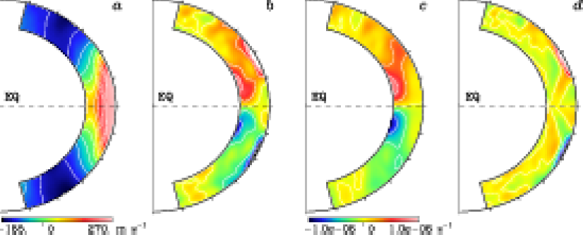
Figure 7.— Temporal and longitudinal average for case $AB$ of ($a$) the longitudinal velocity $\hat{v}_{\phi}$, ($b$) its derivative along the z axis, $\partial\hat{v}_{\phi}/\partial z$, ($c$) the baroclinic term in the meridional force balance (see equation 14), and ($d$) the difference between the last two terms [namely ($b$) minus ($c$)]. The results have been averaged over a period of 275 days. Panel ($d$) shows that there are major departures from a simple thermal-wind balance, especially near the top of the domain. The same color scale is used in panels ($b$), ($c$) and ($d$).

4.2. Baroclinicity and thermal winds

Convection influenced by rotation can lead to latitudinal heat transport in addition to radial transport, thereby producing latitudinal gradients in temperature and entropy even if none were imposed by the boundary conditions. This further implies that surfaces of constant mean density and mean pressure will not coincide, thereby admitting baroclinic terms in the vorticity equations (Pedlosky 1987, Zahn 1992). Baroclinicity has been argued to possibly have a pivotal role in obtaining differential rotation profiles whose angular velocity, like the sun, are not constant on cylinders (e.g. Kitchatinov & Rüdiger 1995). We shall here analyze our cases $AB$ and $C$ from that perspective, finding that though a small latitudinal entropy gradient is realized, the resulting differential rotation as exhibited in our solutions by the mean longitudinal velocity $\hat{v}_{\phi}$ cannot be accounted for principally by the baroclinic term. To make such interpretation specific, we should turn as in Elliott et al. (2000) to the mean (averaged in longitude and time) zonal component of the curl of the momentum equation (2), expressed as

$$\epsilon_{\phi ij}\frac{\partial}{\partial x_{i}}\left(\widehat{v_{k}\frac{\partial v_{j}}{\partial x_{k}}}+\hat{\rho}\,^{-1}\frac{\partial}{\partial x_{k}}\widehat{{\cal D}_{kj}}\right) = 2\,\Omega_{o}\,\frac{\partial\hat{v}_{\phi}}{\partial z}$$

$$+ \hat{\rho}\,^{-2}\mbox{$\nabla$}\,\hat{\rho}\,\mbox{\boldmath$\displaystyle\times$}\mbox{$\nabla$}\,\hat{p}\Bigr{|}_{\phi}\mbox{ ,}$$

where the Einstein summation convention has been adopted, $\epsilon$ represents the permutation tensor, and

$$\frac{\partial}{\partial z}\equiv\cos\theta\frac{\partial}{\partial r}-\frac{\sin\theta}{r}\frac{\partial}{\partial\theta}$$

is the derivative parallel to the rotation axis. This vorticity equation is helpful in examining the relative importance of different forces in meridional planes; here terms arising from Reynolds and viscous stresses are on the left and from Coriolis and baroclinic effects on the right. If one were to simply neglect the Reynolds and viscous stresses, we obtain the simplest version of a ‘thermal–wind balance’ in which departures of zonal winds from being constant on cylinders aligned with the rotation axis are accounted for by the baroclinic term involving crossed gradients of density and pressure, namely

$$2\,\Omega_{o}\,\frac{\partial\hat{v}_{\phi}}{\partial z}=-\hat{\rho}\,^{-2}\mbox{$\nabla$}\,\hat{\rho}\,{\mbox{\boldmath$\displaystyle\times$}}\mbox{$\nabla$}\,\hat{p}\Bigr{|}_{\phi}\mbox{ .}$$ (13)

With the superadiabatic gradient expressed as

$$\frac{1}{c_{P}}\mbox{$\nabla$}\,\hat{S}=\frac{1}{\gamma\hat{p}}\mbox{$\nabla$}\,\hat{p}-\frac{1}{\hat{\rho}}\mbox{$\nabla$}\,\hat{\rho}\mbox{ ,}$$ (14)

where $\gamma$ is the logarithmic derivative of pressure with respect to density at constant specific entropy, we can rewrite equation (13) as

$$\frac{\partial\hat{v}_{\phi}}{\partial z}=\frac{1}{2\Omega_{o}\hat{\rho}c_{P}}\mbox{$\nabla$}\,\hat{S}\,\mbox{\boldmath$\displaystyle\times$}\mbox{$\nabla$}\,\hat{p}\Bigr{|}_{\phi}=\frac{g}{2\Omega_{o}r\,c_{P}}\frac{\partial\hat{S}}{\partial\theta}\mbox{ ,}$$ (15)

having neglected turbulent pressure. Thus breaking the Taylor-Proudman constraint that requires rotation to be constant on cylinders, with $\partial\hat{v}_{\phi}/\partial z$ zero, can be achieved by establishing a latitudinal entropy gradient. However, Reynolds and viscous stresses can also serve to break that constraint, and indeed we next show that those terms are at least as important as the baroclinic term.

Figure 8.— As in Fig. 7, analyzing the role of baroclinicity in the more turbulent case $C$ in maintaining the differential rotation. There are significant departures from a thermal-wind balance in thin regions near the top and bottom of the shell.

We turn in Figure 7 to an analysis of case $AB$ in terms of how well is a simple thermal–wind balance achieved or violated. Figures 7$a,b$ display the temporal mean zonal velocity $\hat{v}_{\phi}$ and its gradient $\partial\hat{v}_{\phi}/\partial z$, with the latter having pronounced variations at mid latitudes near the top of the spherical shell and others at lower latitudes near the bottom of the domain. The baroclinic term [as on right of equation (15)] is shown in Figure 7$c$, possessing the largest amplitudes close to the base of the shell at low latitudes, with a tongue connecting to mid latitudes in traversing the shell. The difference between this baroclinic term and the actual $\partial\hat{v}_{\phi}/\partial z$, as shown in Figure 7$d$, is a measure of the effectiveness of a thermal–wind balance in case $AB$. It is evident that baroclinicity yields a fair semblance of a balance over much of the deeper layer, with the baroclinic term (Fig. 7$c$) typically being greater in amplitude than $\partial\hat{v}_{\phi}/\partial z$ (Fig. 7$b$) there. However, the major regions of departure with opposite signs in the two hemispheres show that in the upper domain, between latitudes of about 15^∘ and 45^∘, that balance is quite severely violated: there the Reynolds stress terms in equation (4.2) involving vortex tube stretching and tilting become the main players. This broad site coincides with regions of strong latitudinal gradient in $\hat{v}_{\phi}$, and is centered in latitude where the relative rotation changes sense from prograde to retrograde. What we have learned from this is that whereas the convection does establish a latitudinal gradient of entropy that is needed for baroclinic terms to achieve aspects of thermal–wind balance over the deeper portions of the domain, the Reynolds stresses have an equally crucial role in the meridional force balance over portions of the upper domain. The more turbulent case $C$ is likewise analyzed in Figure 8, and it generally exhibits comparable behavior. The baroclinic term (Fig. 8$c$) captures much of the $\partial\hat{v}_{\phi}/\partial z$ variation (Fig. 8$b$) at mid latitudes over most of the deep shell, but there are large departures (Fig. 8$d$) in thin domains near the top and bottom of the shell, again between 15^∘ and 45^∘ in latitude. Thus here too the Reynolds stress terms are significant players in the overall balance.

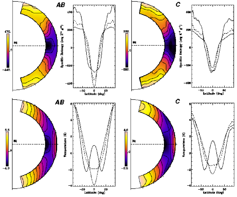
Figure 9.— Temporal and longitudinal averages for cases $AB$ and $C$ of the specific entropy (upper panels) and temperature fluctuations (lower panels), accompanied by latitudinal profiles at the base (dash dotted line), at the middle (dashed) and at the top (solid) of the convective domain. The results have been averaged over periods in turn of 275 and 175 days. The presence of a latitudinal variation of entropy is consistent with the baroclinic term (shown in Figs. 7 and 8) and involves an equator to pole temperature contrast of at most 4 to 8 K near the top where the mean temperature is about $10^{5}$ K.

The latitudinal entropy and temperature gradients established within our simulations should be examined further. We show in Figure 9 the time and longitude averaged specific entropy fluctuations $\hat{S}$ and temperature fluctuations $\hat{T}$ for cases $AB$ and $C$, presenting both color contour renderings across the shell and their variations with latitude at three depths. Our model $AB$, which exhibits the strongest differential rotation, also possesses the greatest temperature and entropy contrasts with latitude. We see from the latitudinal cuts of temperature that a $\Delta\Omega$ of order 30% involves a pole–equator temperature variation of about 4 to 8 degree K, the pole being warmer. These temperature contrasts are very small compared to the mean temperature near the top of our domain of about $10^{5}$ K, and of $2\times 10^{6}$ K near its base. There is some evidence of a latitudinal variation in the photospheric temperature of at least a few K with the same sense obtained from observations of the solar limb (e.g. Kuhn 1998), though relative variations of such small amplitude are very difficult to measure. We note that our temperature fields show some banding with latitude near the top of the domain, with the equator slightly warm, then attaining relatively cool values with minima at about latitude 35^∘, followed by rapid ascent to warm values at high latitudes. The behavior is monotonic with latitude at greater depths, as it is consistently so for entropy at all depths. These differences between temperature and entropy are accounted for by effects of the pressure field necessary to drive the meridional circulation.

In summary, although our solutions attain close to a thermal–wind balance over large portions of the domain, the departures elsewhere are most significant. These arise from the Reynolds stresses that have a crucial role in establishing the differential rotation profiles realized in our simulations. The baroclinicity in our solutions, resulting from latitudinal heat transport that sets up a pole-to-equator temperature and entropy contrast, contributes to $\Omega$ not being constant on cylinders, but it is not the dominant player as envisioned in some discussions of mean-field models of solar differential rotation (e.g. Kitchatinov & Rüdiger 1995, Rekowski & Rüdiger 1998; Durney 1999, 2000).

5. CONCLUSIONS

Our five simulations studying the coupling of turbulent convection and rotation within full spherical shells have revealed that strong differential rotation contrasts can be achieved for a range of parameter values. With these new models, we have focused on two fundamental issues raised in comparing the solar differential rotation deduced from helioseismology with the profiles achieved in the prior 3–D simulations of turbulent convection with the ASH code (Miesch et al. 2000, Elliott et al. 2000). As Issue 1, the sun appears to possess remarkably slow poles, with $\Omega$ decreasing steadily with latitude even at mid and high latitudes (Fig. 1). In contrast, the previous models showed little variation in $\Omega$ at the higher latitudes, having achieved most of their latitudinal angular velocity contrast $\Delta\Omega$ in going from the equator to about 45^∘. As Issue 2, there was a tendency for $\Delta\Omega$ to diminish or even decrease sharply within the prior simulations as the convection became more turbulent, yielding values of $\Delta\Omega$ that were becoming small compared to the helioseismic deductions. In seeking to resolve these two issues, we have explored two paths in parameter space that yield complex and turbulent states of convection. Path 1 involves decreasing the Prandtl number in the sequence of cases $A$, $B$ and $C$, while keeping the Péclet number nearly constant. Path 2 maintains a constant Prandtl number as both the Reynolds and Péclet number are increased in the sequence of cases $AB$, $B$ and $D$. On both paths the convective Rossby number has been chosen to be less than unity, thereby maintaining a strong rotational influence on the convection even as the flows become more intricate.

In dealing with Issue 1, our case $AB$ provides the first indications that it is possible to attain solutions in which the polar regions rotate significantly slower than the mid latitudes (Fig. 4). There is a monotonic decrease from the fast (prograde) equatorial rate in $\Omega$ to the slow (retrograde) rate of the polar regions. Further, that case $AB$ has $\Omega$ nearly constant on radial lines at the higher latitudes, again in the spirit of the helioseismic inferences. We do not fully understand why in case $AB$ such a strikingly different $\Omega$ profile results, compared to that in our other solutions (and of the progenitor simulations) in which the contrast $\Delta\Omega$ is mainly achieved in the lower latitudes. Our principal clues come from Figure 6 where we find that only in case $AB$ is the Reynolds stress component of the net radial angular momentum flux ${\cal F}_{r,R}$ (through shells at various radii) uniformly directed outward. From having examined in detail angular momentum flux streamfunctions (not shown) with radius and latitude consistent with equations (7–9), we observed that the Reynolds stress contributions to such transport possessed multi-celled structures with radius at high latitudes in all the cases except $AB$. The single-cell behavior there for case $AB$ appears to enable more effective extraction of angular momentum by Reynolds stresses from the high to the low latitudes, thereby yielding a distinctive rotational slowing of the high latitudes. Further, case $AB$ possesses strong meridional circulations at low latitudes, but only feeble ones at latitudes above 30^∘, unlike other solutions such as case $C$ (Figs. 3.4, 3.4). This yields a weak meridional component ${\cal F}_{\theta,M}$ (seeking to spin up the poles) to the latitudinal angular momentum flux, thereby allowing the equatorward transport by the Reynolds stress component ${\cal F}_{\theta,R}$ to succeed in extracting angular momentum from the higher latitudes. Such polar slowing also leads to case $AB$ possessing the greatest $\Delta\Omega$ attained in our five simulations (Table $2$).

We also considered the possibility that the slow pole behavior in case $AB$ may have baroclinic origins. This can result from suitable correlations in velocity and thermal structures yielding a latitudinal heat flux which may produce substantial entropy variations at the higher latitudes, thereby leading to greater baroclinic contributions in equation (11) that defines the variation of mean zonal velocity. Examination of Figure 7 at high latitudes does not reveal a prominent baroclinic contribution, and this is consistent with the bland variation of entropy for case $AB$ (Fig. 9) at latitudes above about 40^∘. We conclude that the origin of the slow rotation rate in polar regions appears to be primarily dynamical, being associated with the Reynolds stress transports, and not with baroclinicity that arises from latitudinal heat transport serving to establish a sufficiently warm pole. Although case $AB$ provides a solution that resolves Issue 1, it is unique in achieving this among our five simulations. It may be that in parameter space there only exists a small basin of attraction for such behavior, though we think it more likely that several solution states may coexist for the same control parameters, one of which exhibits the gradual rotational slowing at high latitudes, and others having most $\Omega$ variations confined to low and mid latitudes. We plan to examine whether the slow pole characteristics of case $AB$ can be maintained at nearby sites in parameter space if started from initial conditions corresponding to $AB$, and plan to report on this in the future.

Issue 2 concerns sustaining a strong differential rotation with latitude as the convection becomes more complex. The two paths that we have explored in parameter space to achieve more complex and turbulent states yield relative angular velocity contrasts $\Delta\Omega/\Omega_{o}$ in latitude that are comparable to values deduced from helioseismology, with both our models and apparently the sun possessing a contrast of order 30%. Further, this is accomplished while imposing an upper thermal boundary condition that ensures a uniform emerging heat flux with latitude, as suggested in Elliott et al. (2000). Path 1 involving a decreasing Prandtl number is somewhat more effective in attaining large $\Delta\Omega$ as the solutions become turbulent than Path 2 which has the Prandtl number fixed at 0.25 as both diffusivities are decreased. This holds out hope that even more turbulent solutions will act likewise.

We have shown that the strong $\Delta\Omega$ results from the role of the Reynolds stresses in redistributing the angular momentum. This transport is established by correlations in velocity components arising from convective structures that are tilted toward the rotation axis and depart from the local radial direction and away from the meridional plane. These yield both $v_{r}v_{\phi}$ and $v_{\theta}v_{\phi}$ correlations necessary for the Reynolds stress contributions to the radial and latitudinal angular momentum fluxes analyzed in Figure 6. The fast downflow plumes have a dominant role in such Reynolds stresses, much as seen in local studies (Brummell et al. 1998). Our simulations have attained a spatial resolution adequate to begin to attain coherent structures amidst the turbulence, which is believed to be a key in sustaining strong Reynolds stresses at higher turbulence levels. This has the consequence that all our spherical shells possess fast prograde equatorial rotation relative to the reference frame. There are some contributions toward maintaining the differential rotation from the latitudinal heat transport inherent in our convection that serves to establish a warm pole (with a contrast of a few K) relative to the equator, with baroclinicity and a partial thermal–wind balance helping to yield equatorial acceleration. The meridional circulations generally work to oppose such tendencies by redistributing angular momentum so as to try to spin up the poles. Our simulations on Paths 1 and 2 confirm that strong differential rotation with fast equators has its primary origin in angular momentum transport associated with the Reynolds stresses. Such prominent transports serve to resolve Issue 2. Our next challenge is to satisfy Issue 1 simultaneously with Issue 2 in the more turbulent solutions, which may also lead to $\Omega$ being more nearly constant on radial lines at mid to high latitudes.

Although our results for $\Omega$ have made promising contacts with helioseismic deductions about the state of solar differential rotation in the bulk of the convection zone, there are also major issues that we have not yet tackled. We must evaluate more advanced subgrid-scale terms in representing the unresolved turbulence within such simulations, especially in the near-surface regions. Foremost are also questions of how does the presence of a region of penetration below the convection zone influence the angular momentum redistribution in the primary zone above, and does the tachocline of shear that is established near the interface with the deeper radiative interior modify properties within the convection zone itself. We are keen to also investigate aspects of the rotational shear evident close to the solar surface. This is just now becoming computationally feasible, and involves extending our computational domain upward and beginning to resolve supergranular motions there, as discussed in DeRosa & Toomre (2001) in preliminary studies with thin shells. We are still at early stages with our simulations using ASH to study turbulent convection in spherical shells, yet it is comforting that the mean differential rotation profiles realized in some of the simulations are beginning to capture many of the dominant features for $\Omega$ deduced from the helioseismic probing.

We thank Nicholas Brummell, Marc DeRosa, Julian Elliott, Peter Gilman, Mark Miesch and Jean-Paul Zahn for useful discussions and comments during the writing phase of this paper, and a referee for encouraging us to clarify the objectives and thrust of the presentation. This work was partly supported by NASA through SEC Theory Program grant NAG5-8133 and by NSF through grant ATM-9731676. Various phases of the simulations with ASH were carried out with NSF PACI support of the San Diego Supercomputer Center (SDSC), the National Center for Supercomputing Applications (NCSA), and the Pittsburgh Supercomputing Center (PSC). Much of the analysis of the extensive data sets was carried out in the Laboratory for Computational Dynamics (LCD) within JILA.

Table 1Parameters for the Five Simulations

Case	A	AB	B	C	D
$N_{r},N_{\theta},N_{\phi}$	64, 128, 256	64, 128, 256	64, 256, 512	192, 256, 512	192, 512, 1024
$R_{a}$	3.1 $\times 10^{4}$	3.4 $\times 10^{4}$	1.4 $\times 10^{5}$	3.1 $\times 10^{5}$	6.5 $\times 10^{5}$
$T_{a}$	7.7 $\times 10^{4}$	3.1 $\times 10^{5}$	1.2 $\times 10^{6}$	5.4 $\times 10^{6}$	6.5 $\times 10^{6}$
$P_{r}$	1	0.25	0.25	0.125	0.25
$R_{oc}$	0.645	0.662	0.673	0.682	0.633
$\nu$	5.5 $\times 10^{12}$	2.8 $\times 10^{12}$	1.4 $\times 10^{12}$	6.8 $\times 10^{11}$	6.0 $\times 10^{11}$
$\kappa$	5.5 $\times 10^{12}$	1.1 $\times 10^{13}$	5.5 $\times 10^{12}$	5.5 $\times 10^{12}$	2.4 $\times 10^{12}$
$\tilde{R}_{e}$	28	85	170	385	410
$\tilde{R}_{o}$	0.10	0.16	0.15	0.17	0.16
$\tilde{P}_{e}$	28	21	43	48	103

All simulations have an inner radius $r_{bot}=5.0\times 10^{10}$ cm, an outer radius $r_{top}=6.72\times 10^{10}$ cm, with $L=1.72\times 10^{10}$ cm the thickness of the computational domain. The number of radial, latitudinal and longitudinal mesh points are $N_{r},N_{\theta},N_{\phi}$. Here evaluated at mid-layer depth are the Rayleigh number $R_{a}=(-\partial\rho/\partial S)\Delta SgL^{3}/\rho\nu\kappa$, the Taylor number $T_{a}=4\Omega^{2}L^{4}/\nu^{2}$, the Prandtl number $P_{r}=\nu/\kappa$, the convective Rossby number $R_{oc}=\sqrt{R_{a}/T_{a}P_{r}}$, the rms Reynolds number $\tilde{R}_{e}=\tilde{v}L/\nu$, the rms Péclet number $\tilde{P}_{e}=\tilde{R}_{e}P_{r}=\tilde{v}L/\kappa$, and the rms Rossby number $\tilde{R}_{o}=\tilde{\omega}/2\Omega\sim\tilde{v}/2\Omega L$, where $\tilde{v}$ is a representative rms convective velocity. A Reynolds number based on the peak velocity at mid depth would be about a factor 4 larger. The eddy viscosity $\nu$ and eddy conductivity $\kappa$ at mid depth are quoted in cm${}^{2}\,$s^-1.

Table 2Representative Velocities, Energies and Differential Rotation

	Mid Convective Zone						Volume Average
Case	$\tilde{v}_{r}$	$\tilde{v}_{\theta}$	$\tilde{v}_{\phi}$	$\tilde{v}_{\phi}^{\prime}$	$\tilde{v}$	$\tilde{v}^{\prime}$	KE	DRKE	CKE	MCKE	$\Delta\Omega/\Omega_{o}$
A	46	40	69	44	92	74	2.7$\times 10^{6}$	8.2$\times 10^{5}$ (30%)	1.9$\times 10^{6}$ (70%)	$1.0\times 10^{4}$ (0.37%)	12%
AB	50	47	124	53	142	87	6.5$\times 10^{6}$	4.2$\times 10^{6}$ (64%)	2.3$\times 10^{6}$ (36%)	2.1$\times 10^{4}$ (0.32%)	33%
B	57	56	115	59	140	99	6.5$\times 10^{6}$	3.4$\times 10^{6}$ (52%)	3.1$\times 10^{6}$ (48%)	2.5$\times 10^{4}$ (0.38%)	28%
C	68	67	122	70	155	117	7.9$\times 10^{6}$	3.6$\times 10^{6}$ (46%)	4.3$\times 10^{6}$ (54%)	3.3$\times 10^{4}$ (0.42%)	30%
D	72	67	108	64	146	111	6.5$\times 10^{6}$	2.3$\times 10^{6}$ (35%)	4.2$\times 10^{6}$ (65%)	3.0$\times 10^{4}$ (0.46%)	25%

In the five cases, temporal averages at mid-layer depth in convection zone of rms components of velocity $\tilde{v}_{r}$, $\tilde{v}_{\theta}$, $\tilde{v}_{\phi}$ and of speed $\tilde{v}$, and of fluctuating velocities $\tilde{v}_{\phi}^{\prime}$ and $\tilde{v}^{\prime}$ (with temporal and azimuthal mean subtracted), all expressed in m s^-1. Also listed are the time averages over the full domain of the total kinetic energy, KE, that associated with the (axisymmetric) differential rotation, DRKE, with the (axisymmetric) meridional circulation, MRKE, and with the non-axisymmetric convection itself, CKE, all in erg cm^-3. The relative latitudinal contrast of angular velocity $\Delta\Omega/\Omega_{o}$ between $0^{\circ}$ and $60^{\circ}$ near the top of the domain are stated.

References

- (1) Brandenburg, A., Jennings, R.L., Nordlund, Å., Rieutord, M., Stein, R.F., & Tuominen, I. 1996, J. Fluid Mech., 306, 325
- (2) Braun, D.C., & Fan, Y. 1998, ApJ, 508, L105
- (3) Brummell, N.H., Cattaneo, F., & Toomre, J. 1995, Science, 269, 1370
- (4) Brummell, N.H., Hurlburt, N.E., & Toomre, J. 1996, ApJ, 473, 494
- (5) Brummell, N.H., Hurlburt, N.E., & Toomre, J. 1998, ApJ, 493, 955
- (6) Brummell, N.H., Clune, T.L., & Toomre, J. 2001, ApJ, in press
- (7) Brun, A.S., Turck-Chièze, S., & Zahn, J.-P. 1999, ApJ, 525, 1032
- (8) Brun, A.S., & Toomre, J. 2001, in Helio- and Asteroseismology at the Dawn of the Millenium, ed. A. Eff-Darwich & A. Wilson (Noordwijk: ESA), ESA SP–464, 619
- (9) Canuto, V.M. 1999, ApJ, 524, 311
- (10) Cattaneo, F. 1999, ApJ, 515, L39
- (11) Charbonneau, P., Dikpati, M., & Gilman, P.A. 1999, ApJ, 526, 513
- (12) Chou, D.-Y., & Dai, D.-C. 2001, ApJ, 559, L175
- (13) Choudhuri, A.R., Schüssler, M., & Dikpati, M. 1995 A&A, 303, L29
- (14) Clune, T.L., Elliott, J.R., Glatzmaier, G.A., Miesch, M.S., & Toomre, J. 1999, Parallel Computing, 25, 361
- (15) DeRosa, M.L., & Toomre, J. 2001, in Helio- and Asteroseismology at the Dawn of the Millenium, ed. A. Eff-Darwich & A. Wilson (Noordwijk: ESA), ESA SP–464, 595
- (16) Dikpati, M., & Charbonneau, P. 1999, ApJ, 518, 508
- (17) Durney B.R. 1999, ApJ, 511, 945
- (18) Durney B.R. 2000, ApJ, 528, 486
- (19) Elliott, J.R., Miesch, M.S., & Toomre, J. 2000, ApJ, 533, 546.
- (20) Giles, P.M. 1999, P.D. thesis, Stanford University
- (21) Giles, P.M., Duvall, T.L., Jr., & Scherrer, P.H. 1998, in Structure and Dynamics of the Interior of the Sun and Sun-like Stars, ed. S.G. Korzennik & A. Wilson (Noordwijk: ESA), ESA SP–418, vol. 2, 775.
- (22) Gilman, P.A., & Miller, J. 1981, ApJS, 61, 585
- (23) Gilman, P.A. 2000, Solar Phys., 192, 27
- (24) Glatzmaier, G.A., & Gilman, P. 1982, ApJ, 256, 316
- (25) Glatzmaier, G.A. 1985, ApJ, 291, 300
- (26) Glatzmaier, G.A. 1987, in The Internal Solar Angular Velocity, ed. B. R. Durney & S. Sofia (Dordrecht: D. Reidel), 263
- (27) Gough, D.O. 1969, J. Atmos. Sci., 26, 448
- (28) Gough, D.O., & Toomre, J. 1991, Annu. Rev. Astron. Astrophys., 29, 627
- (29) Gough, D.O., & McIntyre, M. E. 1998, Nature, 394, 755
- (30) Grote, E., & Busse, F.H. 2001, Fluid Dyn. Res., 28, 349
- (31) Haber, D.A., Hindman, B.W., Toomre, J., Bogart, R.S., Schou, J., & Hill, F. 1998, in Structure and Dynamics of the Sun and Sun-like Stars, ed. S.G. Korzennik & A. Wilson (Noordwijk: ESA), ESA SP–418, Vol. 2, 791
- (32) Haber, D.A., Hindman, B.W., Toomre, J., Bogart, R.S., Thompson, M.J., & Hill, F. 2000, Solar Phys., 192, 335
- (33) Haber, D.A., Hindman, B.W., Toomre, J., Bogart, R.S., Larsen, R.M., & Hill, F. 2001, ApJ, in press
- (34) Harvey, J.W. et al. 1996, Science, 272, 1284
- (35) Hathaway, D.H. et al., 1996, Science, 272, 1306
- (36) Hathaway, D.H. et al., 2000, Solar Phys., 193, 495
- (37) Howard, R., Gilman, P.A., & Gilman, P.I., 1984 ApJ, 283, 373
- (38) Howe, R., Christensen-Dalsgaard, J., Hill, F., Komm, R.W., Larsen, R.M., Schou, J., Thompson, M.J., & Toomre, J. 2000a, Science, 287, 2456
- (39) Howe, R., Christensen-Dalsgaard, J., Hill, F., Komm, R.W., Larsen, R.M., Schou, J., Thompson, M.J., & Toomre, J. 2000b, ApJ, 533, L163
- (40) Hurlburt, N.E., Toomre, J., & Massaguer, J.M., 1986, ApJ, 311, 563
- (41) Kichatinov, L.L., & Rüdiger, G. 1995, A&A, 299, 446
- (42) Kuhn, J.R. 1998, in Structure and Dynamics of the Sun and Sun-like Stars, ed. S. G. Korzennik & A. Wilson (Noordwijk: ESA), ESA SP–418, Vol. 2, 871
- (43) Lesieur, M. 1997, Turbulence in Fluids, (Dordrecht: Kluwer)
- (44) Libbrecht, K.G. 1989, ApJ, 336, 1092
- (45) Miesch, M.S. 2000, Solar Phys., 192, 59
- (46) Miesch, M.S., Elliott, J.R., Toomre, J., Clune, T.L., Glatzmaier, G.A., & Gilman, P.A. 2000, ApJ, 532, 593
- (47) Pedlosky, J. 1987, Geophysical Fluid Dynamics, (New York: Springer-Verlag)
- (48) Porter, D.H., & Woodward, P.R. 2000, ApJS, 127, 159
- (49) Porter, D.H., & Woodward, P.R. 2001, ApJ, in preparation
- (50) Rieutord, M., & Zahn, J.-P. 1995, A&A, 296, 127
- (51) Rekowski, B.v., & Rüdiger, G. 1998, A&A, 335, 679
- (52) Robinson, F.J., & Chan, K.L. 2001, MNRAS, 321, 723
- (53) Scherrer, P.H. et al. 1995, Solar Phys., 162, 129
- (54) Schou, J., & Bogart, R.S. 1998, ApJ, 504, L131
- (55) Schou, J. et al. 1998, ApJ, 505, 390
- (56) Schüssler, M. 1987, in The Internal Solar Angular Velocity, ed. B.R. Durney & S. Sofia (Dordrecht: D. Reidel), 303
- (57) Spiegel, E.A., & Zahn, J.-P. 1992, A&A, 265, 106
- (58) Stein, R.F., & Nordlund, Å. 1998, ApJ, 499, 914
- (59) Sun, Z.-P., & Schubert, G. 1995, Phys. Fluids, 7, 2686
- (60) Takehiro, S.-I., & Hayashi, Y.-Y. 1999, Geophys. Astrophys. Fluid Dynam., 90, 43
- (61) Thompson, M.J. et al. 1996, Science, 272, 1300
- (62) Tobias, S.M., Brummell, N.H., Clune, T.L., & Toomre, J. 2001, ApJ, 549, 1183
- (63) Toomre, J., Christensen-Dalsgaard, J., Howe, R., Larsen, R.M., Schou, J., & Thompson, M.J. 2000, Solar Phys., 192, 437
- (64) Ward, F. 1966, ApJ, 145, 416
- (65) Zahn, J.-P. 1992, A&A, 265, 115
- (66) Zahn, J.-P. 2000, Ann. N. Y. Acad. Sci., 898, 90