Fine Tuning in Quintessence Models with Exponential Potentials

Abstract:

We explore regions of parameter space in a simple exponential model of the form $V=V_{0}\ e^{-\lambda\frac{Q}{M_{p}}}$ that are allowed by observational constraints. We find that the level of fine tuning in these models is not different from more sophisticated models of dark energy. We study a transient regime where the parameter $\lambda$ has to be less than $\sqrt{3}$ and the fixed point $\Omega_{Q}=1$ has not been reached. All values of the parameter $\lambda$ that lead to this transient regime are permitted. We also point out that this model can accelerate the universe today even for $\lambda>\sqrt{2}$, leading to a halt of the present acceleration of the universe in the future thus avoiding the horizon problem. We conclude that this model can not be discarded by current observations.

1 Introduction

The universe today is in a stage of accelerated expansion and we still do not know exactly what is the physical mechanism that drives this acceleration. Several alternatives have been proposed, such as the old cosmological constant or the effect of a field whose potential energy dominates nowadays the energy of the universe [1]. This last proposal is usually called quintessence [2].

One of the simplest models for quintessence is a scalar field rolling down an exponential potential [3]. Exponential potentials are natural in theories with extra compact dimensions, such as Kaluza-Klein supergravity and superstring models [4].

Recently, it was pointed out the possibility of having exponential quintessence with a temporary acceleration phase, avoiding the horizon problem that appears in the context of string theory associated with eternal acceleration [5].

Exponential quintessence has been studied extensively in the literature [6, 7] and usually discarded from limits on big-bang nucleosynthesis. This is the motivation for introducing more complex models with, e.g. two scalar fields [8] and double exponential potentials [9]. However, the arguments against the simple exponential model are based on the assumption that a fixed point solution for the quintessence evolution is reached early on in the universe. Therefore, one has to analyse the case where the field have not yet reached this fixed point. This is the goal of this article. We find regions of parameter space for exponential quintessence that are allowed by observational constraints and examine the level of fine tuning required for realistic solutions.

2 Fixed point or fine tuning?

We adopt the potential

$$V(Q)\>=\>V_{0}\ e^{-\lambda\frac{Q}{M_{p}}}\ ,$$ (1)

where $Q$ is the scalar quintessence field, $M_{p}=(8\pi G)^{-1/2}$ is the reduced Planck mass and $\lambda$ and $V_{0}$ are parameters of the potential.

The equation of motion for the quintessence field is given by:

$$\ddot{Q}+3H\dot{Q}\>=\>-\frac{dV}{dQ}\ ,$$ (2)

where dot denotes differentiation with respect to time. Friedmann’s equation for a flat universe is:

$$H^{2}\>=\>\frac{\dot{R}^{2}}{R^{2}}\>=\>\frac{1}{3M_{p}^{2}}\ \left(\rho_{M}+\rho_{R}+\frac{1}{2}\dot{Q}^{2}+V(Q)\right)\ ,$$ (3)

where $R$ is the scale factor and $H$ is the Hubble parameter. For scalar fields, the energy density and pressure are respectively $\rho_{Q}=\frac{1}{2}\dot{Q}^{2}+V(Q)$ and $p_{Q}=\frac{1}{2}\dot{Q}^{2}-V(Q)$. The radiation and matter densities $\rho_{R}$ and $\rho_{M}$ evolve as:

$$\dot{\rho}_{M(R)}+nH\rho_{M(R)}\>=\>0\ ,$$ (4)

with $n=3(4)$ for non-relativistic (relativistic) matter.

The acceleration $\ddot{R}$ of the universe is given by

$$\frac{\ddot{R}}{R}\>=\>-\frac{1}{6M_{p}^{2}}\sum_{i}\rho_{i}\left(1+3\omega_{i}\right),$$ (5)

where $i=M,R$ and $Q$, $\omega_{M}=0$, $\omega_{R}=1/3$ and $\omega_{Q}=p_{Q}/\rho_{Q}$ are the equation of state for matter, radiation and quintessence respectively. The universe is accelerating today if $\omega_{Q0}<-\frac{1}{3}$, assuming that quintessence is currently the dominant component of the energy density. The index $0$ denotes the present epoch.

The dynamics of the quintessence field is obtained by solving the non-linear, coupled differential equations (2) and (3) with appropriate initial conditions. This system of equations has stable fixed points ($fp$) for $\lambda<\sqrt{n}$ with $\Omega_{Q}^{fp}=1$ and $\lambda>\sqrt{n}$ with $\Omega_{Q}^{fp}=\frac{n}{\lambda^{2}}$ [7], where $n$ depends on which background component is more important when the field reaches the fixed point: $n=3(4)$ for matter (radiation). The case $\lambda>\sqrt{n}$ is the selftuning (or scaling) scalar field discussed by Ferreira and Joyce [6] and by Copeland, Liddle and Wands [7]. In this case, however, either the system reaches its non-trivial fixed point early on in the universe and the value of $\Omega_{Q0}$ is too low or the quintessence field energy density contributes too much to the total energy density in the early universe and spoils big bang nucleosynthesis (BBN) predictions. Furthermore, in this selftuning case the universe is not accelerating today, since when the fixed point is reached, $\omega_{Q}$ imitates the dominant background component equation of state (matter today) and consequently $\omega_{Q0}=\omega_{M}=0$ [6, 7]. For these reasons, this solution can be discarded.

The case of interest is given by $\lambda<\sqrt{3}$, in which the quintessence has not yet reached the fixed point regime today but will do it in the future. In other words, $\Omega_{Q}$ is evolving from a small value (in order that quintessence does not spoil BBN) to its value at the fixed point, $\Omega_{Q}^{fp}=1$. In this case, this is not a selftuning solution, but a tracking [10] one, where $\omega_{Q}$ is also frozen with the different value [7]

$$\omega_{Q}^{fp}\>=\>\frac{\lambda^{2}-3}{3}\ ,$$ (6)

being able to accelerate the universe today. Other regimes cannot explain BBN and/or the present acceleration of the universe, when one is using simple exponential potential.

In all quintessence models there arises the so-called cosmic coincidence problem: why is quintessence starting to dominate just now or, in other words, why is the value of quintessence energy density nearly equal to the matter energy density today? No quintessence model has solved this problem until now, since, in order to explain this coincidence, in general one adjusts the potential energy density to make the selftuning (or the tracking) field to freeze in a energy density that is of the order of the critical density today. In [10], for instance, two examples are considered: $V(Q)=K^{(4+\alpha)}Q^{-\alpha}$ and $V(Q)=K^{4}\left[\exp(M_{p}/Q)-1\right]$, where $M_{p}$ is the Planck mass and $K$ is a constant. For any given $V(Q)$, there is a family of tracking solutions parameterized by $K$, whose value is fixed by the measured value of $\Omega_{M0}$. This means that the overall scale of the potential for all quintessence models has to be of the order of the present energy density. For this reason, $K$ is a free parameter used to fit current observations. Whether the order of magnitude of the initial conditions and parameters can be obtained in reasonable physical models is a very important question that has not been fully answered in a satisfactory manner.

Hence, because the cosmic coincidence problem has not been explained by any quintessence model, what one can do is to discuss the naturalness of the choice of initial conditions and parameters. Our goal in this article is exactly this: we study what is the size of the region in parameter space and how precisely adjusted these initial conditions and parameters must be in order to explain some observational constraints, that is, what amount of fine tuning is necessary in simple exponential when one requires that it has not yet reached its fixed point regime.

3 Relevant equations

We will follow closely the approach described in Cline [5]. Instead of integrating in time, we will use another variable $u$ defined by:

$$u\>\equiv\>\ln(1+z)\>=\>-\ln R/R_{0}\ ,$$ (7)

where $z$ is the redshift, and we take $R_{0}=1$. We also define new dimensionless variables:

$$\hat{Q}\>\equiv\>\frac{1}{\sqrt{3}M_{p}}\ Q\ ,\qquad\qquad\hat{\rho}_{i}\>\equiv\>\frac{1}{3M_{p}^{2}(H_{0}^{m})^{2}}\rho_{i}\ ,$$ (8)

$$\hat{V}\>\equiv\>\frac{1}{3M_{p}^{2}(H_{0}^{m})^{2}}\ V\ ,\qquad\qquad\qquad\hat{H}\>\equiv\>\frac{H}{H_{0}^{m}}\ ,$$ (9)

where $H_{0}^{m}=100h_{0}$ km s^-1 Mpc^-1 is the currently measured Hubble parameter and therefore:

$$3M_{p}^{2}(H_{0}^{m})^{2}\>=\>\rho_{c0}^{m}=\>1.88\times 10^{-29}\ h_{0}^{2}\ \ \mathrm{g/cm^{3}}\ .$$ (10)

The dimensionless variables $\hat{\rho}_{i}$ and $\hat{V}$ are given in terms of the critical density. In our numerical investigations, we adopt the following values, for $h_{0}=0.7$:

$$\hat{\rho}_{M0}\>=\>\frac{\rho_{M0}}{\rho_{c0}^{m}}\>=\>0.3\ \ \ \ \ \mathrm{and}\ \ \ \ \ \hat{\rho}_{R0}\>=\>\frac{\rho_{R0}}{\rho_{c0}^{m}}\>=\>4.3\times 10^{-5}h_{0}^{-2}\>=\>8.5\times 10^{-5}\ .$$ (11)

The variable $\hat{H}$ is determined by the numerical solution $H$ of Friedmann’s equation (3) divided by $H_{0}^{m}$.

In terms of the new variables, the potential is given by

$$\hat{V}(\hat{Q})\>=\>\hat{V}_{0}\ e^{-\sqrt{3}\lambda\hat{Q}}\ ,$$ (12)

and the differential equations read:

$$\hat{H}^{2}\hat{Q}^{\prime\prime}-\left(\hat{\rho}_{R}+\frac{3}{2}\hat{\rho}_{M}+3\hat{V}\right)\hat{Q}^{\prime}+\frac{d\hat{V}}{d\hat{Q}}\>=\>0\ ;$$ (13)

$$\hat{H}^{2}\>=\>\frac{\hat{\rho}_{M}+\hat{\rho}_{R}+\hat{V}}{1-\frac{1}{2}\hat{Q^{\prime}}^{2}}\ ;$$ (14)

where prime denotes differentiation with respect to $u$. This corrects a typographical error in Cline [5], where he writes $\hat{V}$ instead of $3\hat{V}$ in equation (13). Notice that because the universe is flat, one is able to isolate $\hat{H}$ in Friedmann’s equation.

These are supplemented by the solutions for the evolution of matter and radiation

$$\hat{\rho}_{M}\>=\>\hat{\rho}_{M0}\ e^{3u}\ ,$$ (15)

and

$$\hat{\rho}_{R}\>=\>\hat{\rho}_{R0}\ e^{4u}\ ,$$ (16)

where $\rho_{R0}$ and $\rho_{M0}$ are the radiation and matter energy densities today. The quintessence energy density is given by:

$$\hat{\rho}_{Q}\>=\>\frac{1}{2}\ \hat{H}^{2}\hat{Q^{\prime}}^{2}+\hat{V}\ .$$ (17)

With these new variables, one can also write

$$\Omega_{i}\>=\>\frac{\rho_{i}}{\rho_{c}}\>=\>\frac{\rho_{i}}{3M_{p}^{2}H^{2}}\>=\>\frac{\hat{\rho}_{i}}{\hat{H}^{2}}\ .$$ (18)

that always satisfy

$$\Omega_{R}+\Omega_{M}+\Omega_{Q}\>=\>1\ .$$ (19)

From the equation above, one can see that the values of $\Omega_{M0}$, $\Omega_{R0}$ and $\Omega_{Q0}$ (since the universe is flat) depends on the solution of Friedmann’s equation. The values (11) used to solve the equations will correspond to the measured values of $\Omega_{M0}$ and $\Omega_{R0}$ only if $H_{0}=H_{0}^{m}$.

The equation of state for quintessence is given by:

$$\omega_{Q}\>=\>\frac{\dot{Q}^{2}-2V}{\dot{Q}^{2}+2V}\>=\>\frac{\hat{H}^{2}\hat{Q^{\prime}}^{2}-2\hat{V}}{\hat{H}^{2}\hat{Q^{\prime}}^{2}+2\hat{V}}\ .$$ (20)

4 Numerical Results

4.1 Parameters

As stated before, in all quintessence models there is an overall constant ($\hat{V_{0}}$ in our case) that is determined by the fact that the major contribution to the energy of the field today must come from the potential term, and that the energy density of quintessence is approximately equal the present measured critical density (more precisely, the critical energy density minus the matter plus radiation energy densities). This work does not aim to discuss the naturalness of such a choice of $\hat{V_{0}}$. We simply follow the same approach used in all quintessence models to “solve” the cosmic coincidence problem.

From equation (20) one sees that the pressure-to-density ratio (equation of state) has a current negative value only if the major contribution for the energy density of the quintessence field comes from the potential term. The observational fact that $\Omega_{Q0}\approx\rho_{c0}^{m}$ implies that

$$V(0)\>=\>V_{0}\ e^{-\sqrt{3}\lambda\hat{Q}_{0}}\>\approx\>\rho_{c0}^{m}\>\approx\>(10^{-3}\mbox{eV})^{4}\ ,$$ (21)

where $V(0)$ denotes the present value of the potential energy density. The value of $V_{0}$ depends on the value of $\hat{Q}_{0}$. As long as the initial condition $\hat{Q^{\prime}}_{i}$ is small (and we will see that this is the case from the equipartition of energy) and the field has not yet reached the fixed point, one can see that $\hat{Q}_{0}\approx\hat{Q}_{i}$, as figure 1 illustrates. Therefore, the values of $V_{0}$ and $\hat{Q}_{i}$ are related by equation (21).

In this sense, the only free parameter in this model is $\lambda$. As mentioned above, we will be interested in the range $0\leq\lambda<\sqrt{3}$, since this region is the only one able to explain all observational constraints.

Figure 1: Value of the field $\hat{Q}$ as function of $u$. For the initial conditions showed, the field has approximately the same features. The field remains almost constant until it reaches the fixed point regime, when it starts to roll-down the potential with a constant derivative in $u$. The initial conditions used along the text are showed by solid line. These curves were made with $\hat{V}_{0}=1$ and $\lambda=1.3$.

4.2 Initial Conditions

In order to solve the differential equations, two extra parameters are needed, namely the initial conditions $\hat{Q}_{i}$ and $\hat{Q^{\prime}}_{i}$. We are interested in the case in which the field has not yet entered in the fixed point regime. In this case, the field has today almost the same value it had initially, and one is able to relate $V(0)$ and $\hat{Q}_{i}$, in such a way that $\hat{Q}_{i}$ can be absorbed in the definition of $\hat{V}_{0}$. For this reason, we will take, with no loss of generality, $\hat{Q}_{i}=0$. We will discuss later the role of $\hat{Q}_{i}$ in the solution. In fact, changing the value of $\hat{Q}_{i}$ just corresponds to a rescaling of the problem.

The freedom in the choice of $\hat{Q}_{i}$ also comes from the fact that the potential energy does not contribute to the initial value of density parameter of the field, $\Omega_{Q,i}$. This can be seen by noticing that $V(0)$ is of the order of the critical density today (see equation (21)) and that our initial conditions are taken at $z\approx 10^{13}$. This implies that $\hat{V_{0}}$ is at least 39 orders smaller than the energy density scale (critical density) of that epoch, since $\rho_{c}\propto H^{2}\propto R^{-3}\ (R^{-4})$ during matter (radiation) domination epoch. The initial energy of the field is then in the form of kinetic energy, or

$$\Omega_{Q,i}\>\approx\>\frac{1}{2}\hat{Q^{\prime}}_{i}^{2}\ .$$ (22)

We have assumed a flat universe, which implies that $|\hat{Q^{\prime}}|\leq\sqrt{2}$. The equation above shows what would be needed in order to have the limit case $|\hat{Q^{\prime}}|=\sqrt{2}$ : the dominant energy of the universe must be the kinetic energy of the field.

Natural initial conditions from equipartition of energy after inflation suggests that $\Omega_{Q,i}\simeq 10^{-3}$ [10]. From equation (22) one has then $\hat{Q^{\prime}}_{i}\approx 0.05$.

Therefore, the most likely set of initial conditions are the values $\hat{Q}_{i}=0$ and $\hat{Q^{\prime}}_{i}=0.05$. Nevertheless, we will also study the effect of taking all the possible set of initial conditions, namely $\hat{Q}_{i}\geq 0$ and $0\leq|\hat{Q^{\prime}}_{i}|\leq\sqrt{2}$.

4.3 Constraints

We evaluate the equations and demand that the solutions must satisfy some observational constraints. The first is given by nucleosynthesis. Nucleosynthesis predictions claims [11] that at $95$% confidence level:

$$\Omega_{Q}(1\mbox{MeV}\approx z=10^{10})\>\leq\>0.045\ .$$ (23)

Another observational constraint is given by the quintessence density parameter. Observations from cosmic background radiation anisotropy indicate that the universe is flat. A set of complementary observations indicates that $\Omega_{M0}=0.3\pm 0.1$ [12]. Thus,

$$\Omega_{Q0}\>=\>0.7\pm 0.1\ .$$ (24)

The uncertainty on $\Omega_{M0}$ implies that there is an uncertainty on the determination of $\hat{V}_{0}$. This is the reason why one can study a region on parameter space $(\hat{V}_{0},\lambda)$ in spite of the fact that $\hat{V}_{0}$ is not a free parameter.

The last observational constraint considered here is the present quintessence equation of state [12]:

$$-1\>\leq\>\omega_{Q0}\>\leq\>-0.6\ .$$ (25)

The fact that the universe is accelerating today, as will be shown in figure 4, does not imply that it will accelerate forever. The present value of equation of state of quintessence in the cases studied in this work is temporary, since the equation of state is frozen only when the field reaches the fixed point regime, what will happen in near future.

4.4 Results and Discussion

We solve numerically the coupled differential equations (13,14) using equations (12,15,16). The effect of all possible initial conditions will be discussed later. First, however, the particular choice (the most likely one) of initial conditions $\hat{Q}_{i}=0$ and $\hat{Q^{\prime}}_{i}=0.05$ will be studied.

For this set of initial conditions, the region of parameter space able to satisfy all observational constraints, contrary to common belief, is reasonable, varying from $\lambda=0$ to $\lambda\approx 1.7$ and from $\hat{V}_{0}\approx 0.5$ to $\hat{V}_{0}\approx 3.0$. In other words, all possible values of $\lambda$ in the tracking regime are able to satisfy the present observational constraints. The results are shown in figure 2.

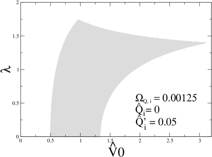
Figure 2: Region of parameter space that satisfies all observational constraints discussed in subsection 4.3. There is a reasonable region of parameters of the exponential potential that can explain all observations. In fact, all values of $\lambda$ that produce the tracking solutions satisfy the constraints. The uncertainty on $\hat{V}_{0}$ comes from the uncertainty on $\Omega_{M0}$.

Figures 3, 4 and 5 shows respectively how the energy densities, the equation of state of quintessence and density parameters varies with $u$. Initially, quintessence contributes to a small fraction of energy of the universe and decreases as $R^{-6}$, dominated by the kinetic term ($\omega_{Q}=1$), faster than matter and radiation densities. When the potential term becomes important, there is a rapid change in the equation of state from $\omega_{Q}=1$ to $\omega_{Q}=-1$ and the quintessence density freezes until today, when it becomes dominant. Afterwards, the quintessence reaches the fixed point regime, which is characterised by the quintessence density parameter going from as small value at $u\approx 2.5$ and reaching the fixed point, $\Omega_{Q}^{fp}=1$, when $u\approx-2.5$. In the fixed point regime (tracking solution), the ratio between kinetic and potential energy densities becomes constant and consequently $\omega_{Q}^{fp}$ is given by the equation (6). In this regime, the energy density decreases as $R^{-3(1+\omega_{Q}^{fp})}=R^{-\lambda^{2}}$.

Figure 4 shows the behavior of equation of state for various parameters. Initially they have the same behavior, but they evolve differently after quintessence enters the fixed point regime, because different parameters correspond to different frozen ratios between kinetic and potential energy densities. $\lambda$ is the parameter that determines what value $\omega_{Q}^{fp}$ will be frozen in: small values of $\lambda$ corresponds to small values of $\omega_{Q}^{fp}$ and vice versa. In particular, for $\lambda>\sqrt{2}$ the universe stops to accelerate in the tracking solution, since $\omega_{Q}^{fp}>-\frac{1}{3}$ in these cases. For small values ($\lambda\lesssim 0.15$) the quintessence behaves like a cosmological constant in the tracking solution.

Figure 3: Energy density as function of $u$ for quintessence, matter and radiation for a typical solution. Initially quintessence density decreases faster than matter and radiation. When the potential term becomes important, $\hat{\rho}_{Q}$ freezes. When the fixed point regime (tracking solution) is reached, the field changes again its behavior and decreases as $R^{-\lambda^{2}}$, lower than matter. Plot made with parameters $\hat{V}_{0}=1$ and $\lambda=1.3$.

Figure 4: Equation of state as function of $u$ for various parameters. Initially all have the same behavior. When quintessence reaches its fixed point, each solution is frozen in a specific value, depending mainly on $\lambda$: small values of $\lambda$ correspond to smaller values of $\omega_{Q}^{fp}$ and vice versa. For a small $\lambda$, quintessence behaves in the fixed point regime like a cosmological constant. For $\lambda>\sqrt{2}$, the universe does not accelerate in this regime.

Figure 5: Density parameters of quintessence, matter and radiation. The fixed point regime is characterised by quintessence density parameter equal to unity ($\Omega_{Q}^{fp}=1$). The fixed point solution was not yet reached today, which is a transition epoch. The parameters used were $\hat{V}_{0}=1$ and $\lambda=1.3$.

The correlation between the free parameter $\lambda$ and the equation of state today is shown in figure 6. Notice that there is a degeneracy for $\lambda\gtrsim 0.6$, namely, different values of $\lambda$ generate the same $\omega_{Q0}$. This degeneracy is mainly due the fact that the present value of equation of state is not its value in the fixed point regime, since the tracking solution was not yet reached. In the fixed point regime the degeneracy does not exist, since equation (6) is satisfied.

Figure 6: Allowed region of ($\lambda,\omega_{Q0}$) space. Notice that $\omega_{Q0}\leq-0.6$, according to constraint (25). This plot is independent on values of $\hat{V}_{0}$ and $\hat{Q}_{i}$ and changes only for “high” values of $\hat{Q^{\prime}}_{i}$ ($\hat{Q^{\prime}}_{i}\gtrsim 1.25$). The fact that different values of $\lambda$ are able to give the same $\omega_{Q0}$ comes from the fact that today the fixed point regime was not yet reached.

With better measurements of $\omega_{Q0}$, one could put severe constraints on the exponential potential model, specially if $\omega_{Q0}\lesssim-0.85$. This is the region of low $\lambda$ and, as it was commented before, in this region quintessence behaves as a cosmological constant today. It is important to realize that the figure 6 remains the same for almost all sets of values of $\hat{V}_{0}$, $\hat{Q}_{i}$ and $\hat{Q^{\prime}}_{i}$ that are able to produce a tracking solution we are interested here, since the value of equation of state depends mainly on $\lambda$. In fact, in order to have this plot unchanged, it is enough that exists a considerable region of $\lambda$ in the parameter space ($\hat{V}_{0},\lambda$). Later will be shown that the existence of this region only depends on $\hat{Q^{\prime}}_{i}$. Only for values of $\hat{Q^{\prime}}_{i}\gtrsim 1.25$ this plot will be changed.

Another important aspect is the dependence of these results on $\hat{Q}_{i}$. Figure 7 shows the region of parameter space that satisfies all observational constraints when one uses as initial conditions $\hat{Q}_{i}=1$ and $\hat{Q^{\prime}}_{i}=0.05$. When $\hat{Q}_{i}\neq 0$, the region of parameter space is deformed in $\hat{V}_{0}$ by a factor of $e^{\sqrt{3}\lambda\hat{Q}_{i}}$, because in these models $\hat{V}_{0}$ can always be rescaled as $\hat{v}_{0}=\hat{V}_{0}e^{-\sqrt{3}\lambda\hat{Q}_{i}}$, since $\hat{Q}_{0}\approx\hat{Q}_{i}$. Hence, in this sense, choosing another value of $\hat{Q}_{i}$ corresponds to just a rescaling of the “old” region.

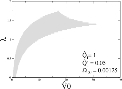
Figure 7: Region of parameter space that satisfies all observational constraints, when one is using as initial conditions $\hat{Q}_{i}=1$ and $\hat{Q^{\prime}}_{i}=0.05$. Note that using $\hat{Q}_{i}\neq 0$ just corresponds to rescale the parameter space in $\hat{V}_{0}$ by a factor of $e^{\sqrt{3}\lambda\hat{Q}_{i}}$.

As it was seen in equation (22), the initial condition $\hat{Q^{\prime}}_{i}$ corresponds to the initial value of density parameter of quintessence. The most likely value is $\hat{Q^{\prime}}_{i}=0.05$ because of the energy equipartition after inflation. However, one can argue that choosing this value could also be a fine tuning. For this reason, it is important to explore what happens with the allowed region of the parameter space if $\hat{Q^{\prime}}_{i}$ has a different value, keeping in mind that $0\leq|\hat{Q^{\prime}}_{i}|\leq\sqrt{2}$. The results are shown in figure 8.

The region of parameter space becomes smaller in $\hat{V}_{0}$ when $\hat{Q^{\prime}}_{i}$ increases. This happens because the field has to satisfy the constraint (23). When the density parameter of quintessence is large initially, in general the density parameter of quintessence contributes too much to the total energy density during the BBN epoch, and a smaller region of parameter space is able to satisfy the observational constraints. Nevertheless, a reasonable region of parameter space still exists for almost all values of $\hat{Q^{\prime}}_{i}$. In fact, the region of parameter space only vanishes when $\Omega_{Q,i}\gtrsim 0.75$. In other words, for almost all possible values of $\hat{Q^{\prime}}_{i}$ in a flat universe there still is a significant region of the parameter space able to satisfy all observational constraints.

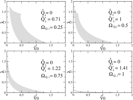
Figure 8: Regions of parameter space for various $\hat{Q^{\prime}}_{i}$ different from that of inflationary equipartition. Since the universe is flat, $|\hat{Q^{\prime}}_{i}|\leq\sqrt{2}$. For almost all possible values of $|\hat{Q^{\prime}}_{i}|$ a significant region on parameter space still exists. It only vanishes for $\Omega_{Q,i}\gtrsim 0.75$.

5 Conclusion

In this work we have studied the simplest quintessence model with an exponential potential. This potential is usually discarded because it cannot satisfy simultaneously all observational constraints. This is true in a regime where the field has already reached its fixed point regime. We have studied this model in a regime where the field has not yet reached its fixed point regime (tracking solution) today. We have shown that, contrary to common belief, this potential is able to satisfy all observational constraints for a reasonable region of parameter space ($\hat{V}_{0},\lambda$).

We have also shown that the resulting parameters and initial conditions are not unnatural. On the contrary, we showed that these parameters and initial conditions are not less natural than that used for other models of quintessence. For almost all possible values of $\hat{Q^{\prime}}_{i}$ there still is a significant allowed region of parameter space. $\hat{V}_{0}$ is determined by the measured value of $\Omega_{M0}$, the same feature used in all quintessence models. $\hat{Q}_{i}$ does not affect qualitatively the region of parameter space, since in the regime in which the field has not entered its tracking solution $\hat{Q}_{i}$ and $\hat{V}_{0}$ are related, and consequently $\hat{Q}_{i}$ just rescales the problem. The only free parameter of this model is $\lambda$, which determines the behavior of the field. All values of $\lambda$ that produce the tracking solution satisfy the observational constraints. Depending on $\lambda$, the universe may or may not accelerate forever.

The allowed regions that we found are essentially due to present experimental uncertainties: the region of $\hat{V}_{0}$ is due the uncertainties on measured value of $\Omega_{M0}$ and the region on $\lambda$ arises from the observational uncertainties on $\omega_{Q0}$. If the uncertainties were reduced, these regions would also be reduced. In this case, one would be able to determine the values of the parameters of the simple exponential potential using observations.

This potential cannot be discarded by any of the constraints discussed here, even if better measurements were made. The only way to discard this potential based on the constraints discussed in this work would be if constraint of BBN (23) had been more stringent. For example, if one had showed that $\Omega_{Q}(1\mathrm{MeV})\leq 10^{-6}$, probably the region of parameter space would become smaller, in such way that could not be possible to explain the measured value of $\omega_{Q0}$, for example. Another way to discard this potential is to include another constraint as, for instance, the value of $\Omega_{Q}$ during the epoch of formation of structure or in the last scattering surface, and verify that this model is not able to satisfy all constraints simultaneously. Therefore, we showed that at the moment there is no reason to discard the exponential potential or to consider it less natural than any other quintessence model.

- [1] For recent reviews, see e. g. V. Sahni, The Cosmological Constant Problem and Quintessence, Class. Quant. Grav. 19, 3435 (2002) [astro-ph/0202076]; S. M. Carroll, The Cosmological Constant, Living Rev. Rel. 4, 1 (2001) [astro-ph/0004075] and references therein.
- [2] R. R. Caldwell, R. Dave and P. J. Steinhardt, Cosmological Imprint of an Energy Component with General Equation of State, Phys. Rev. Lett. 80, 1582 (1998) [astro-ph/9708069].
- [3] B. Ratra and P. J. E. Peebles, Cosmological Consequences of a Rolling Homogeneous Scalar Field, Phys. Rev. D37, 3406 (1988); C. Wetterich, Cosmology and the Fate of Dilatation Symmetry, Nucl. Phys. B302, 668 (1988).
- [4] See, e.g., J. Halliwell, Scalar Fields in Cosmology with an Exponential Potential, Phys. Lett. B185, 341 (1987); Q. Shafi and C. Wetterich, Inflation from Higher Dimensions, Nucl. Phys. B289, 787 (1987) .
- [5] J. M. Cline, Quintessence, Cosmological Horizons, and Selftuning, JHEP 0108, 035 (2001) [hep-ph/0105251]; C. Kolda and W. Lahneman, Exponential Quintessence and the End of Acceleration, hep-th/0105300.
- [6] P. G. Ferreira and M. Joyce, Structure Formation with a Selftuning Scalar Field, Phys. Rev. Lett. 79, 4740 (1997) [astro-ph/9707286]; Cosmology with a Primordial Scaling Field, Phys. Rev. D58, 023503 (1998) [astro-ph/9711102].
- [7] E. J. Copeland, A. R. Liddle and D. Wands, Exponential Potentials and Cosmological Scaling Solutions, Phys. Rev. D57, 4686 (1998)[gr-qc/9711068].
- [8] See, e. g., M. C. Bento, O. Bertolami and N. C. Santos, A Two Field Quintessence Model, Phys. Rev. D65, 067301 (2002) [astro-ph/0106405].
- [9] T. Barreiro, E. J. Copeland and N. J. Nunes, Quintessence Arising from Exponential Potentials, Phys. Rev. D61, 127301 (2000) [astro-ph/9910214].
- [10] P. J. Steinhardt, L. Wang, I. Zlatev, Cosmological Tracking Solutions, Phys. Rev. D59, 123504 (1999) [astro-ph/9812313]; I. Zlatev, L. Wang, P. J. Steinhardt, Quintessence, Cosmic Coincidence, and the Cosmological Constant, Phys. Rev. Lett. 82, 896 (1999) [astro-ph/9807002].
- [11] R. Bean, S. H. Hansen, A. Melchiorri, Constraining the Dark Universe, Nucl. Phys. Proc. Suppl. 110, 167 (2002) [astro-ph/0201127].
- [12] See e. g. L. Wang, R. R. Caldwell, J. P. Ostriker, P. J. Steinhardt, Cosmic Concordance and Quintessence, Astrophys. J. 530, 17 (2000) [astro-ph/9901388].