Star Formation in Bright Rimmed Clouds. I. Millimeter and Submillimeter Molecular Line Surveys

Abstract

We present the results of the first detailed millimeter and submillimeter molecular line survey of bright rimmed clouds, observed at FCRAO in the CO ($J={1}\rightarrow{0}$), C¹⁸O ($J={1}\rightarrow{0}$), HCO⁺ ($J={1}\rightarrow{0}$), H¹³CO⁺ ($J={1}\rightarrow{0}$), and N₂H⁺ ($J={1}\rightarrow{0}$) transitions, and at the HHT in the CO ($J={2}\rightarrow{1}$), HCO⁺ ($J={3}\rightarrow{2}$), HCO⁺ ($J={4}\rightarrow{3}$), H¹³CO⁺ ($J={3}\rightarrow{2}$), and H¹³CO⁺ ($J={4}\rightarrow{3}$) molecular line transitions. The source list is composed of a selection of bright rimmed clouds from the catalog of such objects compiled by Sugitani et al. (1991). We also present observations of three Bok globules done for comparison with the bright rimmed clouds. We find that the appearance of the millimeter CO and HCO⁺ emission is dominated by the morphology of the shock front in the bright rimmed clouds. The HCO⁺ ($J={1}\rightarrow{0}$) emission tends to trace the swept up gas ridge and overdense regions which may be triggered to collapse as a result of sequential star formation. Five of the seven bright rimmed clouds we observe seem to have an outflow, however only one shows the spectral line blue-asymmetric signature that is indicative of infall, in the optically thick HCO⁺ emission. We also present evidence that in bright rimmed clouds the nearby shock front may heat the core from outside-in thereby washing out the normally observed line infall signatures seen in isolated star forming regions. We find that the derived core masses of these bright rimmed clouds are similar to other low and intermediate mass star forming regions.

1 Introduction

Triggered Star Formation is the process by which star formation is initiated or accelerated through compression of a clump in a molecular cloud by a shock front (Elmegreen, 1992). Although a basic understanding of the process of triggered star formation exists, only recently have numerical models becoming sophisticated enough to yield detailed comparisons with observations. Comparison of hydrodynamic shock induced star formation models to observations of potential triggered star formation regions is complicated by the fact that such regions can be very chaotic. Shocks, outflows, and core rotation all have kinematic signatures which may overwhelm the signatures associated with the triggering mechanism (Elmegreen, 1998). In order to alleviate this confusion somewhat, we choose to observe regions of potential small scale triggering. These regions typically involve one core in a cometary cloud, and a well defined shock front geometry.

Several numerical studies of shock triggered collapse have been undertaken recently (Boss, 1995; Foster & Boss, 1996, 1997; Vanhala & Cameron, 1998, hereafter VC). These studies have found that shocks with velocities less than 45 km s^-1 can cause cores to collapse, but fast shocks ($>100$ km s^-1) tend to destroy the principal cooling molecules, leading ultimately to the destruction of the cloud . These models also yield an appreciable number of binary and multiple star systems, which are common in our galaxy, yet difficult to form by spontaneous, isolated star formation. The VC models tend to reproduce characteristics of observed cometary clouds thought to be small scale triggered star formation regions (Elmegreen, 1992, 1998). This comparison between the models and the observations will be explored further in a forthcoming paper.

In order to perform a detailed study of sites of triggered star formation, which can be compared to models, we conducted a survey of bright rimmed clouds identified by Sugitani et al. (1991, hereafter, SFO). These are all molecular clouds which border expanding HII regions. At the boundary between the ionized gas within the Stromgren sphere, and the molecular cloud is an ionization front, which shows up as the bright rim identified by SFO. Embedded near the rim, and just within the molecular cloud in each of these sources is an IRAS source. The fact that the ionization front is collecting gas into a ridge or core in many of these sources makes them excellent candidates for the globule squeezing or collect and collapse mode of triggered star formation (Elmegreen, 1992, 1998). These clouds are also divided into three morphological types, shown schematically in Figure 1. The first is type A, which has a moderately curved rim, and looks much like a shield in three dimensions. The second is type B, which has a more tightly curved rim near the head of the cloud, but which tends to broaden near the tail. Type B is also known as an elephant trunk morphology. The third is type C which has a very tightly curved rim and a well defined tail. Type C is often called a cometary cloud. The shock induced collapse models of VC as well as observations of the expanding ionization front of the Orion OB 1 association (Ogura & Sugitani, 1998) suggest that these morphological types of bright rimmed clouds may actually be a time evolution sequence with clouds evolving from type A through type B to type C.

2 Observational Approach

2.1 Source Selection

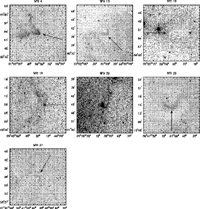
Figure 2: Digitized Sky Survey Image of SFO objects. These images show 20^′ by 20^′ sections of the sky centered on the embedded IRAS object. SFO used these images to classify these objects into their morphological scheme. The arrows indicates the direction of motion of the ionization front.

Potential triggered star formation regions have been selected from the catalog of bright-rimmed clouds with associated IRAS point sources by SFO. Each of these sources is associated with an HII region and is suspected to be forming stars via triggering. In all of these sources the geometry of the incoming shock region is obvious, as the shock emanates from the interface of the cloud and HII region. Since there are three different morphologies, or bright rim cloud types, we decided to chose at least two of each type. We also chose nearby sources, both to get the best possible resolution, and because most Bok globules that have been studied have been nearby objects. The bright rimmed clouds we observed have distances between 190 and 1900 pc, and include two type A bright rimmed clouds (SFO 16 and SFO 18), three type B bright rimmed clouds (SFO 4, SFO 13, and SFO 25), and two type C bright rimmed clouds (SFO 20 and SFO 37). We cannot hope to resolve the cores of the more distant sources with single dish millimeter or submillimeter observations, however we do resolve the structure of the swept up molecular gas cloud surrounding the core, which is greatly affected by the impacting ionization front. The embedded IRAS sources in the selected bright rimmed clouds have infrared luminosities which range from 5 to 1300 $L_{\odot}$, though all but one of the sources have a luminosity less that 110 $L_{\odot}$. These luminosities tend to be typical of low or intermediate mass star formation. Finally all but one of the bright rimmed clouds were chosen to have the IRAS colors of their embedded IRAS point source be consistent with Young Stellar Objects (YSOs) according to the color criteria presented in Beichman (1985). There are two exceptions to this rule. The first, SFO 4, was chosen because it is exceptionally nearby (190 pc). The second, SFO 13, was chosen because it is thought to be a region of cluster formation (Carpenter et al., 2000). Although SFO 4 and SFO 13 do not meet the IRAS color criteria of Beichman (1985) for inclusion in the population of YSOs, they do meet the criteria of Carpenter et al. (2000) for embedded star forming regions. Digitized Sky Survey observations of the bright rimmed clouds are shown in Figure 2. In most of the optical images the bright rim is clearly visible, enclosed within the rim is the molecular cloud. Several of the sources show high extinction on one side of the rim indicating the presence of the molecular cloud. We have drawn in an arrow indicating the direction of propagation of the ionization front from the ionizing source creating the HII region.

In order to compare potential triggered star formation regions with quiescent star formation regions, we also observed Bok globules with embedded IRAS sources in their cores from the Clemens & Barvainis (1988) catalog of small, optically selected molecular clouds. We chose Bok globules with properties that are similar to our bright rimmed clouds. They lie at distances between 250 and 2500 pc from us. They are believed to contain one star forming core with an embedded IRAS source, and their luminosities between 3 and 930 $L_{\odot}$. Observations of these sources allow for detailed comparisons between the observed properties of triggered and spontaneous star formation regions, and will allow us to isolate those observed properties unique to triggered star formation. The three Bok globules we have observed are B335, CB 3, and CB 224. The source list is summarized in table 1.

2.2 Choice of Molecular Transitions

One cannot obtain a complete picture of the physical conditions in a star forming cloud by observing one molecular line. It is only by combining observations of several molecular line transitions, sensitive to various physical conditions, that one can approach an accurate physical representation of the star forming cloud. As a result we chose several molecular transitions, in both the millimeter and submillimeter wave bands, in order to probe the conditions we felt would provide us with a basis for comparing bright rimmed clouds with Bok globules. The transitions we observed are summarized in table 2.

CO has traditionally been the main tracer of molecular clouds. It has a fairly high abundance and a low critical density, making it a very useful tracer of molecular gas. Our observations of CO were driven by the fact that both the CO ($J={1}\rightarrow{0}$) and the CO ($J={2}\rightarrow{1}$) emission are good tracers of molecular outflows. HCO⁺is a good tracer of moderate density ($\geq 10^{4}$ cm^-3). We observe the millimeter HCO⁺ ($J={1}\rightarrow{0}$) line to trace the morphology of the molecular gas swept up by the ionization front. The submillimeter HCO⁺ ($J={3}\rightarrow{2}$) and HCO⁺ ($J={4}\rightarrow{3}$) trace the denser clumps within the swept up gas. HCO⁺emission in all three tracers tends to be optically thick in the cores, making it a good tracer of infall as discussed in §5.3. N₂H⁺ has been shown to be a good tracer of the dense core material as it can only form in well-shielded regions (Turner, 1995). N₂H⁺ also remains relatively undepleated in cores (Bergin & Langer, 1997), making it especially useful in probing the densest regions of star forming clouds. The N₂H⁺ ($J={1}\rightarrow{0}$) transition has seven well measured hyperfine components resulting from the interaction of the molecular electric field gradient and the electric quadrupole moments of the nitrogen nuclei (Caselli et al., 1995). These components can be used to determine the optical depth of N₂H⁺ from which we can derive the column density of N₂H⁺. From this measurement we can infer the density of star forming cores.

2.3 Presentation of the Data

In §4 we will discuss our observations of each source in a systematic way. This section describes the order in which various observations will be described and also points out various features which we look for in these sources. For each source we present figures illustrating the line profiles at the IRAS source position, an integrated intensity map of each tracer which we mapped, a map of the centroid velocity of the HCO⁺ ($J={1}\rightarrow{0}$) transition, and a map of the molecular outflow if one is detected. Our rationale for presenting these figures is discussed below.

We begin by presenting the central line profiles of all the observed molecular transitions. These profiles are taken at the position of the IRAS source. There are several features in the line profiles which are of interest to us. The CO lines often have broad low intensity features called wings. These wings, which are especially prominent in the CO ($J={2}\rightarrow{1}$) transition, are usually the result of an outflow from the forming protostellar object. These outflows are often bipolar and are thought to arise from megnetohydrodynamic winds driven by infall and interaction with the forming star’s surrounding disk (see Bachiller (1996) and references therein). The shape of the line profile can also be of interest. The HCO⁺ transitions often have profiles which deviate significantly from gaussian shapes at line center. This is due to the high optical depth which results in self-absorption near the line center. Often this results in a profile with two distinct peaks. When this is indeed the result of self-absorption, the lower abundance H¹³CO⁺ lines are often still optically thin and tends to show their greatest intensity at a velocity between the twin peaks of their self-absorbed isotopomer HCO⁺. The relative size of each peak often indicates the kinematics of the gas within the beam. When the gas is collapsing to a point within the beam, the red-shifted gas is preferentially self-absorbed leaving a more intense blue-shifted peak and an overall blue-asymmetry with respect to the H¹³CO⁺ line. The reverse is true for gas expanding from a point within a beam (Snell & Loren, 1977; Zhou, 1992, 1995).

The integrated intensity maps provide a look at the two-dimensional morphology of the molecular cloud and cores as seen by the different tracers we mapped over the region surrounding the IRAS sources. The CO integrated intensity map gives a global look at the molecular gas in the region. One thing to note in the bright rimmed clouds we observe is that the boundary between the molecular cloud and the ionized gas is very sharp and well traced by the CO. The HCO⁺ tends to trace denser regions, but is also excited by shocks (Bachiller & Pérez Guitiérrez, 1997). As a result HCO⁺ ($J={1}\rightarrow{0}$) tends to trace both the star forming cores as well as the rim of the ionization front. The higher level HCO⁺ transitions tend to trace the dense gas. We overlay the N₂H⁺ half-power contour on the integrated intensity map of a higher level HCO⁺ transition in order to show the correspondence between the dense gas traced by N₂H⁺ and that traced by HCO⁺. There is often good agreement between the two tracers. Following the integrated intensity maps we present HCO⁺ ($J={1}\rightarrow{0}$) centroid velocity maps for most of the sources. Centroid velocity maps have been shown to be very effective in disentangling the underlying velocity fields in regions of complex kinematics (Narayanan & Walker, 1998). Often there is a velocity gradient which may correspond to rotation of the cloud or be a result of acceleration of the molecular gas due to the rocket effect which arises at the molecular cloud boundary.

The kinematic signature suggested by the HCO⁺ is often interesting when compared to the integrated intensity maps of the CO outflows, which we present next for many of the sources we observe. Often the bipolar outflow we detect in CO is perpendicular to the velocity gradient we detect in HCO⁺. This is evidence that we may be detecting rotation along the direction predicted in current models of star formation. We do not have the angular resolution, however, to probe this rotation down to the small scales of the star forming core.

3 Observations

3.1 FCRAO 14m

We performed observations at the Five College Radio Astronomy Observatory (FCRAO) 14 m telescope over the 1999–2000 and 2000–2001 observing seasons using the Second Quabbin Observatory Imaging Array (SEQUOIA) 16-beam array receiver, and the Focal Plane Array Autocorrelation Spectrometers (FAAS) which consists of 16 autocorrelating spectrometers. A summary of the observed molecular line transitions is shown in table 2. The C¹⁸O, HCO⁺, H¹³CO⁺, and N₂H⁺ transitions were observed using the frequency-switched mode, while CO was observed by position switching to a region that was reasonably clear of CO emission, though some CO contamination was found and considered acceptable in the offset positions as long as it was well separated in velocity from the line of interest. The HCO⁺and H¹³CO⁺ were frequency folded and 3^rd order baselines were removed, while for the N₂H⁺ data a 4^th order baseline was used. A 2^nd order baseline was subtracted from the position-switched CO data. HCO⁺ and N₂H⁺ were mapped with half-beam spacing, while CO and H¹³CO⁺ were mapped with full-beam spacing. The extent of the region mapped varies depending on the spatial extent of the source’s emission.

3.2 HHT 10m

We also performed submillimeter observations in April and December 2000 and in April 2001 with the 10 m Heinrich Hertz Telescope (HHT). CO $J={2}\rightarrow{1}$, HCO⁺, and H¹³CO⁺$J={3}\rightarrow{2}$ observations were conducted using the facility 230 GHz SIS receiver, while HCO⁺ and H¹³CO⁺ observations were conducted using the facility dual polarization 345 GHz SIS receiver. Several backends were used simultaneously, including a 1 GHz wide ($\sim 1$ MHz resolution) acousto-optical spectrometer (AOS), and three filterbanks with 1 MHz, 250 kHz, and 62.5 kHz resolutions. The results presented in this paper were processed using the 250 kHz filterbank. All observations were position-switched, and second order baselines were removed. H¹³CO⁺ observations were made of the star forming core at the IRAS source position, while HCO⁺ and CO observations were made using the on-the-fly (OTF) mapping technique. Observations of $120\mbox{${}^{\prime\prime}$}\times 60\mbox{${}^{\prime\prime}$}$ regions in OTF mode were combined into maps of various spatial extents depending on the source.

3.3 CSO 10.4m

We observed B335 in May of 1996 at the Caltech Submillimeter Observatory (CSO). HCO⁺ ($J={4}\rightarrow{3}$) mapping was performed using the OTF mapping technique. The OTF data was gridded into 49 positions with a spacing of 10^′′. H¹³CO⁺ ($J={4}\rightarrow{3}$) was observed at the IRAS source position. All observations were carried out with low-noise SIS waveguide receivers and a 1000 channel, 50 MHz wide acousto-optical spectrometer. The main beam efficiency at 345 GHz is $\sim 0.65$. Calibration of observations was done by the chopper wheel technique.

4 Results

4.1 Bright Rimmed Clouds

4.1.1 SFO 4

SFO 4 is a bright rimmed cloud with a type B morphology on the edge of the HII region S185 ($\gamma$ Cas) (SFO). IRAS source 00560+6037 is embedded within SFO 4. This IRAS source has been classified by SFO as having IRAS colors consistent with hot cirrus sources, and not a forming or newly formed star (SFO). However according to the criteria of Carpenter et al. (2000) SFO 4 fits the IRAS color profile of an embedded star forming region. SFO 4 is nearby (190 pc), and has no known associated outflows or HH objects.

Figure 3a shows the spectra of our observations towards the IRAS source in SFO 4. Although H¹³CO⁺ ($J={1}\rightarrow{0}$) was not detected, our observations limit the integrated intensity of that transition to less that 0.037 K km s^-1. Based on this limit, and the integrated intensity measurement of HCO⁺ ($J={1}\rightarrow{0}$), and an assumed C/¹³C abundance ratio of 64 we derive an upper limit to the column density of HCO⁺ to be $2\times 10^{13}$ cm^-2. The line profiles appear fairly gaussian, in all the observed transitions, with nearly identical centroid velocities. None of the isotopic lines of either CO or HCO⁺ were detected.

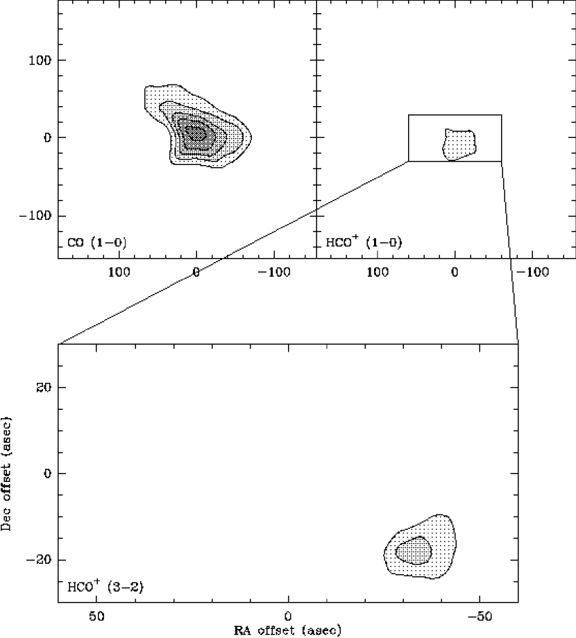
Figure 4: Integrated intensity maps of SFO 4 in various transitions and isotopomers of HCO⁺and CO. The IRAS source 00560+6037 is located at the center of each map. The CO ($J={1}\rightarrow{0}$) map has a lowest contour of 1.9 K km s^-1 ($3\sigma$) and increments of 1.3 K km s^-1 ($2\sigma$). The HCO⁺ ($J={1}\rightarrow{0}$) map has a lowest contour of 0.6 K km s^-1 ($3\sigma$) and increments of 0.2 K km s^-1 ($1\sigma$). The HCO⁺ ($J={3}\rightarrow{2}$) map has a lowest contour of 0.7 K km s^-1 ($2\sigma$) and increments of 0.3 K km s^-1 ($1\sigma$).

Figure 4 shows the HCO⁺ and CO integrated intensity maps. Neither the CO ($J={1}\rightarrow{0}$) map, nor the HCO⁺ maps show much structure. In the CO ($J={1}\rightarrow{0}$) map and the HCO⁺ ($J={1}\rightarrow{0}$) map the cloud core surrounding the embedded IRAS source is visible, but no gas traces the ionization front or the elephant trunk morphology seen in the DSS image in Figure 2. The HCO⁺ ($J={3}\rightarrow{2}$) map shows only one point whose integrated intensity is above 1.0 K km s^-1, the three sigma threshold for the map. This source is unusually weak compared to the other sources in the sample, which is unfortunate as it is also the most nearby source in the sample.

4.1.2 SFO 13

SFO 13 is classified as a type B bright rimmed cloud by SFO. Figure 2 shows the elephant trunk morphology characteristic of type B clouds. The initially cometary head of the cloud broadens into a wider structure as one follows the cloud away from the ionizing source. SFO 13 borders the HII region IC1848, and lies at a distance of 1.9 kpc from us, making it the most distant SFO source in the sample. A recent near-infrared survey reveals $\sim 20$ point sources whose spectral energy distributions are consistent with pre-main-sequence stars (Sugitani et al., 1995, 1999). $K^{\prime}$ band observations by Carpenter et al. (2000) also confirm the presence an embedded stellar cluster in this molecular cloud. These sources are distributed preferentially towards the HII region with respect to the IRAS source, and are probably older than the IRAS source indicating that this cloud may be an example of small scale sequential star formation.

The millimeter and submillimeter line profiles for SFO 13, shown in Figure 3b, are all fairly gaussian and also peak at approximately the same velocity. This is not entirely unexpected as the average infall region for individual cores in a star formation region is smaller than the FCRAO beamwidth, which is 0.5 pc at this distance, and the HHT beamwidth, of 0.3 pc, making it difficult to detect infall. The CO ($J={2}\rightarrow{1}$) line strength is almost twice as much as that of CO ($J={1}\rightarrow{0}$). This intensity difference may be due to excitation effects, but may also be the result of the small angular size of the core. Since the CO ($J={2}\rightarrow{1}$) transition is observed with a much smaller beam than the CO ($J={1}\rightarrow{0}$) transition, the beam dilution is much greater for the lower transition and can have significant effects on the intensities observed with such distant sources. The HCO⁺ and C¹⁸O line profiles are all fairly gaussian. N₂H⁺ ($J={1}\rightarrow{0}$) was not detected in this source, down to an rms level of 0.017 K km s^-1.

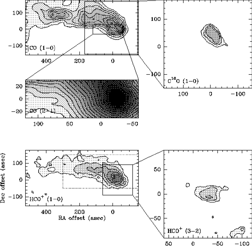
Figure 5: Integrated intensity maps of SFO 13 in various transitions and isotopomers of HCO⁺and CO. The IRAS source 02570+6028 is located at the center of each map. The CO ($J={1}\rightarrow{0}$) map has a lowest contour of 4.6 K km s^-1 ($3\sigma$) and increments of 4.6 K km s^-1 ($3\sigma$). The CO ($J={2}\rightarrow{1}$) map has a lowest contour of 2.1 K km s^-1 ($3\sigma$) and increments of 5.0 K km s^-1 ($7\sigma$). The C¹⁸O ($J={1}\rightarrow{0}$) map has a lowest contour of 0.6 K km s^-1 ($3\sigma$) and increments of 0.2 K km s^-1 ($1\sigma$). The HCO⁺ ($J={1}\rightarrow{0}$) map has a lowest contour of 0.4 K km s^-1 ($3\sigma$) and increments of 0.4 K km s^-1 ($3\sigma$). The HCO⁺ ($J={3}\rightarrow{2}$) map has a lowest contour of 1.7 K km s^-1 ($3\sigma$) and increments of 0.6 K km s^-1 ($1\sigma$). The dotted rectangle in the HCO⁺ ($J={1}\rightarrow{0}$) map indicates the region over which the HCO⁺ centroid is shown in Figure 6.

Although the spatial resolution of our observations are not good enough to trace individual infall regions, the overall gas morphology is resolved by the beam. Figure 5 shows integrated intensity maps of various transitions and isotopes of CO and HCO⁺. The CO ($J={1}\rightarrow{0}$) shows a distinct head, located at the IRAS source position upon which the map is centered. Lower intensity CO ($J={1}\rightarrow{0}$) emission continues from the core and spreads out to the north-east of the image, similar to the elephant trunk morphology seen in the optical (Figure 2). This is also consistent with the fact that the ionizing source is located to the south-west of the core. The region mapped in CO ($J={2}\rightarrow{1}$) shows a similar morphology to the CO ($J={1}\rightarrow{0}$) emission, however the core position is much more intense than the surrounding gas. The C¹⁸O ($J={1}\rightarrow{0}$) map shows emission mostly north of the HCO⁺ core, with very little north-east extension. This indicates that the large column density molecular gas may not correspond exactly with the star forming core in this source.

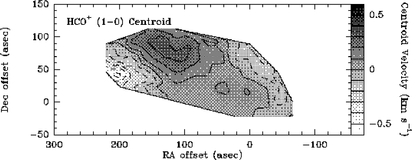
Figure 6: The SFO 13 centroid velocity integrated over the line core of HCO⁺ ($J={1}\rightarrow{0}$). The line of sight velocity has been subtracted out and the contours and greyscale are indicated on the wedge to the right of the figure.

The HCO⁺ ($J={1}\rightarrow{0}$) integrated intensity map (Figure 5) shows a more cometary morphology than the digitized sky survey image in Figure 2. The dense gas appears to be preferentially located along a ridge near the southern edge of the cloud. This could be a result of the preexisting density structure of the molecular cloud which was swept up by the ionization front or an effect of the geometry of the expanding HII region. However, these observations can not determine how the gas was swept into that ridge. The HCO⁺ ($J={3}\rightarrow{2}$) integrated intensity map only shows significant emission at the position of the star forming core. The HCO⁺ ($J={1}\rightarrow{0}$) centroid map (Figure 6) does not show a very coherent structure, however there is a significant velocity gradient across the tail in the HCO⁺ ($J={1}\rightarrow{0}$) map along the northwest-southeast direction. The CO ($J={2}\rightarrow{1}$) line profiles show distinct wings, which seem to form two lobes of an outflow (Figure 7). This outflow has not previously been observed, although SFO found line wings indicative of an outflow in their CO ($J={2}\rightarrow{1}$) observation of this source.

4.1.3 SFO 16

SFO 16, also known as L1634 and RNO40, is classified as a type A bright rimmed cloud by SFO, as it is a broad ionization front, with no tail. SFO 16 borders Barnard’s Loop, and is at a distance of 400 pc. The embedded IRAS source 05173–0555 has a spectral energy distribution in the IRAS bands consistent with an embedded YSO (SFO). Cohen (1980) describes this object as a purely nebulous elongated very Red source typical of Herbig-Haro objects. Emission lines which Cohen (1980) detects in this source include H$\alpha$, H$\beta$, H$\gamma$, [NII], [SII], [OI], [NI], [OIII], and HeI.

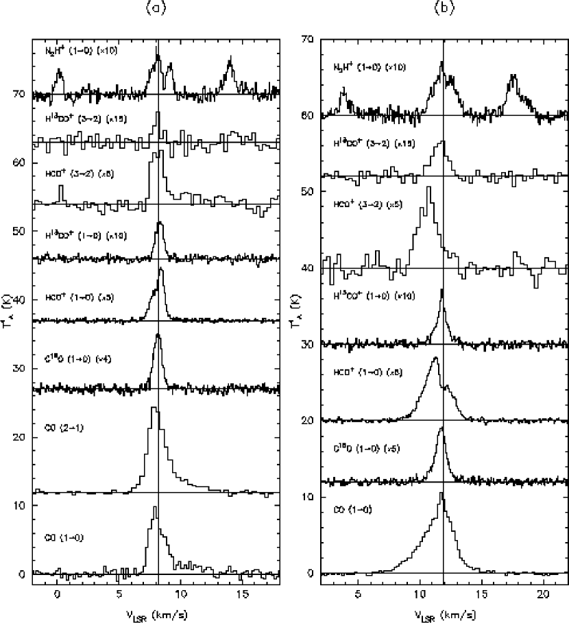
Figure 8: Line profiles of molecular transitions in the direction of the central IRAS source of SFO 16 (a) and SFO 18 (b).

Figure 8a shows the central line profiles towards the IRAS source 05173–0555. The vertical line indicates the best fit velocity of the N₂H⁺ ($J={1}\rightarrow{0}$) hyperfine ensemble. Both the CO ($J={1}\rightarrow{0}$) and the CO ($J={2}\rightarrow{1}$) lines show wings. These wings often indicate the presence of outflows. The C¹⁸O ($J={1}\rightarrow{0}$) line, however appears to have a fairly gaussian shape. The HCO⁺ line profiles, shown in Figure 8a, are a bit more enigmatic. The HCO⁺ ($J={3}\rightarrow{2}$) and H¹³CO⁺ ($J={3}\rightarrow{2}$) lines seem fairly well centered on the $V_{\rm LSR}$, but the HCO⁺ ($J={1}\rightarrow{0}$) shows a pronounced asymmetry. This asymmetric profile is not shared by the H¹³CO⁺ ($J={1}\rightarrow{0}$) line, indicating that the asymmetry observed in the HCO⁺ line is probably the result of a radiative transfer effect, and not an effect of the superposition of clouds along the line of sight. Line asymmetries can be produced by infall (Walker et al., 1994), however this produces a line which has greater emission blue-shifted from line center, and our example is red-shifted from line center. It is possible that the HCO⁺ ($J={1}\rightarrow{0}$) profile is caused by an outflow. Another possibility is that this red-asymmetric profile is due to infall in a region where the shock heating has inverted the excitation temperature profile of the infalling gas, so that is has a higher excitation temperature far from the core and a lower excitation temperature near the core. This hypothesis will be fully explored in §5.3.

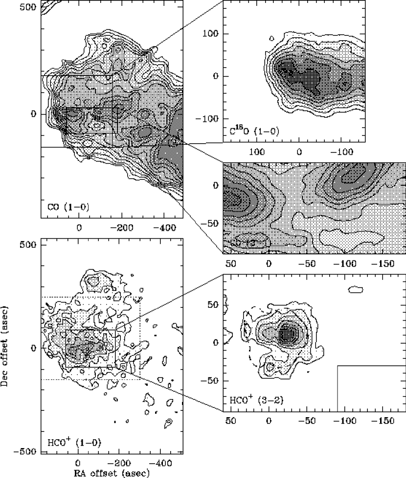
Figure 9: Integrated intensity maps of SFO 16 in various transitions and isotopomers of HCO⁺and CO. The IRAS source 05173–0555 is located at the center of each map. The CO ($J={1}\rightarrow{0}$) map has a lowest contour of 4.3 K km s^-1 ($3\sigma$) and increments of 1.4 K km s^-1 ($1\sigma$). The CO ($J={2}\rightarrow{1}$) map has a lowest contour of 6.0 K km s^-1 ($12\sigma$) and increments of 2.5 K km s^-1 ($5\sigma$). The C¹⁸O ($J={1}\rightarrow{0}$) map has a lowest contour of 0.6 K km s^-1 ($3\sigma$) and increments of 0.2 K km s^-1 ($1\sigma$). The HCO⁺ ($J={1}\rightarrow{0}$) map has a lowest contour of 0.4 K km s^-1 ($3\sigma$) and increments of 0.3 K km s^-1 ($2\sigma$). The HCO⁺ ($J={3}\rightarrow{2}$) map has a lowest contour of 0.9 K km s^-1 ($3\sigma$) and increments of 0.3 K km s^-1 ($1\sigma$). The dotted rectangle in the HCO⁺ ($J={1}\rightarrow{0}$) map indicates the region over which the HCO⁺ centroid is shown in figure 10. The dashed contour in the HCO⁺ ($J={3}\rightarrow{2}$) indicates the half power contour of the N₂H⁺ ($J={1}\rightarrow{0}$) emission.

The CO and HCO⁺ integrated intensity maps are shown in Figure 9. Although classified as a type A cloud by SFO, the CO ($J={1}\rightarrow{0}$) seems to show a well defined tail moving off to the south-west, however the ionization source is located directly to the east of the core. The C¹⁸O ($J={1}\rightarrow{0}$) integrated intensity map (Figure 9) shows the molecular core surrounding the IRAS source, and no evidence of the outflow lobes. It does appear that there is a tail traced by the C¹⁸O elongated to the west of the core. The HCO⁺ ($J={1}\rightarrow{0}$) integrated intensity image in Figure 9 is more indicative of a type A morphology that the CO integrated intensity maps. The majority of the gas traced by the HCO⁺ emission is in a fairly broad regions which is densest around the IRAS core, but shows another possible core 300^′′ north of the IRAS core. The HCO⁺ ($J={3}\rightarrow{2}$) integrated intensity map highlights the location of the core. Figure 10 shows the centroid velocity of the HCO⁺ ($J={1}\rightarrow{0}$) emission in the dense regions of the source. This centroid was calculated over the line core velocities, and do not include contributions from line wings if they are present. On average there appears to be a north-south velocity gradient which could indicate rotation of the cloud.

In both the CO ($J={1}\rightarrow{0}$) and CO ($J={2}\rightarrow{1}$) integrated intensity maps, lobes indicative of a bipolar outflow are evident. Figure 11 shows an integrated intensity map of the CO ($J={2}\rightarrow{1}$) line wings. This figure shows that there is an outflow, with the blue shifted lobe on the west side of the core and the red shifted lobe to the east of the core. Previous studies by Hodapp & Ladd (1995) and Fukui (1989) indicate the presence of this outflow and a second outflow, which we do not detect, aligned in the northwest-southeast direction. The axis of rotation, derived from the HCO⁺ centroid map, is aligned east-west, matching the alignment of outflow we detect. This alignment is predicted by current star formation theories that posit that outflows are located along the polar direction of a rotating protostar, in order to shed some angular momentum before material can fall into the protostar.

4.1.4 SFO 18

SFO 18, also known as B35A, is also a type A bright rimmed cloud . It borders the HII region $\lambda$ Ori at a distance of about 400 pc. The embedded IRAS source 05417+0907 has a spectral energy distribution consistent with an embedded YSO . Myers et al. (1988) have detected an outflow in CO ($J={1}\rightarrow{0}$) which extends in the northwest-southeast direction around the embedded IRAS source.

Our line profiles shown in Figure 8b show bright, extensive wings on the CO ($J={1}\rightarrow{0}$) line, when compared to its C¹⁸O counterpart. The HCO⁺ ($J={1}\rightarrow{0}$) and HCO⁺ ($J={3}\rightarrow{2}$) line profiles both show a significant blue asymmetry when compared to their H¹³CO⁺ isotopic counterparts. This may indicate that the gas is infalling around the core or cores (Walker et al., 1994).

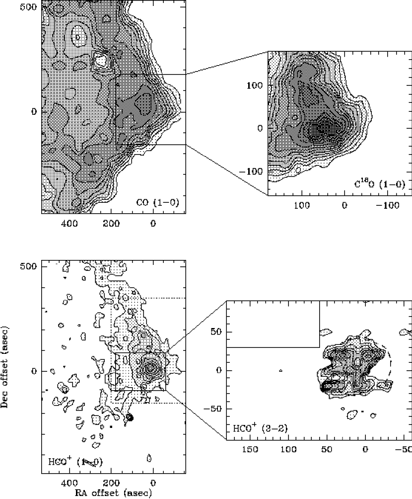
Figure 12: Integrated intensity maps of SFO 18 in various transitions and isotopomers of HCO⁺and CO. The IRAS source 05417+0907 is located at the center of each map. The CO ($J={1}\rightarrow{0}$) map has a lowest contour of 1.8 K km s^-1 ($3\sigma$) and increments of 1.8 K km s^-1 ($3\sigma$). The C¹⁸O ($J={1}\rightarrow{0}$) map has a lowest contour of 0.4 K km s^-1 ($3\sigma$) and increments of 0.1 K km s^-1 ($1\sigma$). The HCO⁺ ($J={1}\rightarrow{0}$) map has a lowest contour of 0.7 K km s^-1 ($3\sigma$) and increments of 0.5 K km s^-1 ($2\sigma$). The HCO⁺ ($J={3}\rightarrow{2}$) map has a lowest contour of 1.6 K km s^-1 ($3\sigma$) and increments of 0.5 K km s^-1 ($1\sigma$). The dotted rectangle in the HCO⁺ ($J={1}\rightarrow{0}$) map indicates the region over which the HCO⁺ centroid is shown in figure 13. The dashed contour in the HCO⁺ ($J={3}\rightarrow{2}$) indicates the half power contour of the N₂H⁺ ($J={1}\rightarrow{0}$) emission.

The CO $J={1}\rightarrow{0}$ integrated intensity map (Figure 12) shows the broad ionization front with a core at its apex, typical of type A sources. The CO emission cuts off fairly abruptly on the western edge of the cloud, where the ionization front is located. The ionizing source is located directly to the west of the core. Besides the increased emission at the core, one can see a general increase in CO ($J={1}\rightarrow{0}$) emission adjacent to the ionization front which is probably due to an increase in column density as gas gets swept up by the ionization front, a factor which ultimately enhances the density and leads to self-gravitating clumps (Elmegreen, 1992). The C¹⁸O ($J={1}\rightarrow{0}$) better traces the high column density gas around the core and shows what may be another core to the northeast of the first. The HCO⁺ ($J={1}\rightarrow{0}$) emission better traces the dense ridge, as seen in the integrated intensity map in Figure 12, and the core in which the IRAS source is embedded. This ridge of dense gas is consistent with the type A morphological classification by . Higher resolution HCO⁺ ($J={3}\rightarrow{2}$) observations of the core show several emission peaks, indicating that there may be several low mass stars forming simultaneously in that region. This is consistent with models of shock driven collapse (Vanhala & Cameron, 1998) in which multiple stars can be formed.

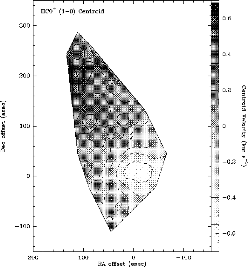
Figure 13: The SFO 18 centroid velocity integrated over the line core of HCO⁺ ($J={1}\rightarrow{0}$). The line of sight velocity has been subtracted out and the contours and greyscale are indicated on the wedge to the right of the figure.

Further evidence supporting a region of infall is seen in Figure 13 where we see that the entire core region has blue shifted HCO⁺ ($J={1}\rightarrow{0}$) centroid velocities relative to the rest of the cloud where emission is strong enough to accurately measure a centroid. This match between the core emission and the region of possible infall is further evidence of a collapsing, star forming, core (Narayanan et al., 2002). Figure 14 shows the integrated intensity map of the CO ($J={1}\rightarrow{0}$) line wings, and we see the outflow in the same direction as detected by Myers et al. (1988).

4.1.5 SFO 20

SFO 20 is a type C bright rimmed cloud. The long tail is visible in the optical image (Figure 2) pointing northwards, away from the HII region IC434, which is approximately 400 parsecs from us . The infrared spectral energy distribution of this source is consistent with an embedded YSO . Sugitani et al. (1989) discovered and mapped an outflow around the embedded IRAS source in SFO 20 using the NRO 45m telescope in the CO ($J={1}\rightarrow{0}$) transition.

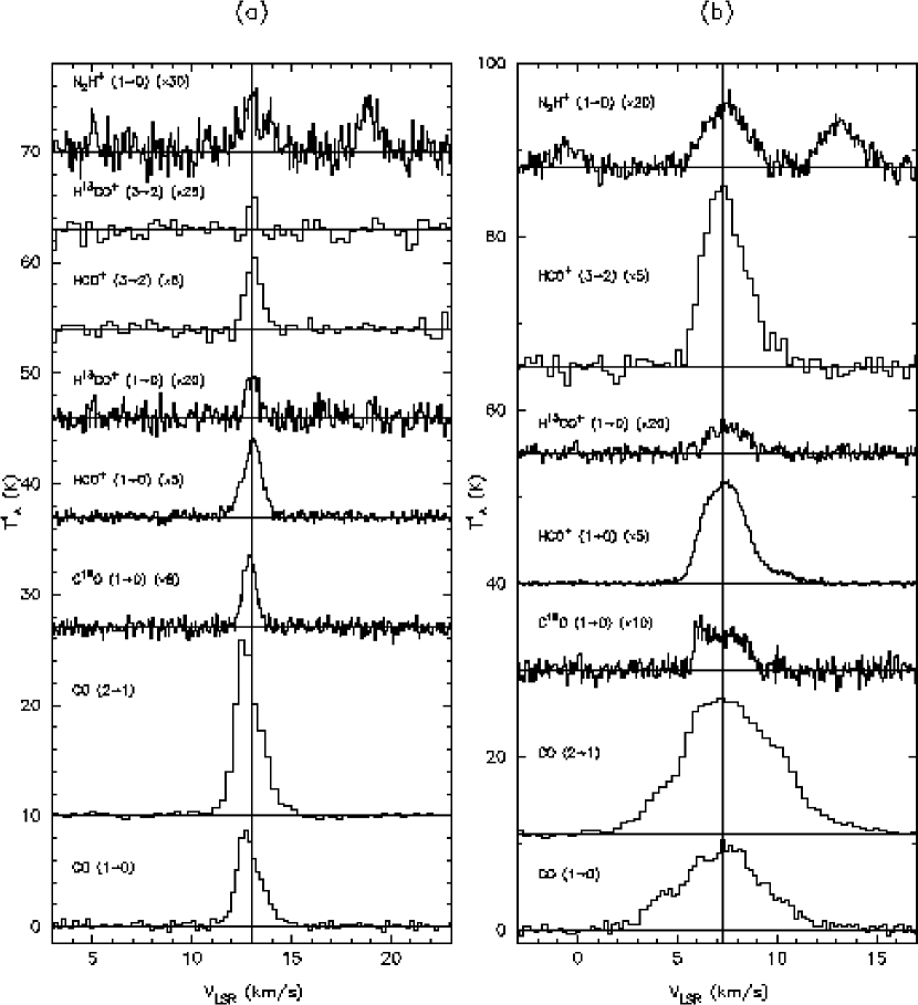
Figure 15: Line profiles of molecular transitions in the direction of the central IRAS source of SFO 20 (a) and SFO 25 (b).

The CO ($J={1}\rightarrow{0}$) and CO ($J={2}\rightarrow{1}$) line profiles shown in Figure 15a show a blue asymmetry and wings on the $J={2}\rightarrow{1}$ transition. The HCO⁺ line profiles are all fairly gaussian, and fairly well centered on the N₂H⁺ ($J={1}\rightarrow{0}$) $V_{\rm LSR}$. There is no clear evidence of infall from the HCO⁺ transitions.

The CO ($J={1}\rightarrow{0}$) integrated intensity map (Figure 16) shows the type C morphology, with a strong core and evidence of a tail trailing off to the north. The CO ($J={2}\rightarrow{1}$) emission also traces the core, though the emission peak does not match the HCO⁺ ($J={3}\rightarrow{2}$) core position exactly. The C¹⁸O ($J={1}\rightarrow{0}$) emission is also peaked on the core and relatively absent in the tail. The HCO⁺ ($J={1}\rightarrow{0}$) emission is mainly centered on the core with some emission tracing the tail. While many of the previous sources had substantial emission outside of the core region, this one does not. Under the assumption that the type C morphology is the most temporally evolved morphology, the ionization front may have long since passed this region and it is surrounded by ionized gas. As the core gas collapses the tail can be eaten away as it becomes less and less shielded. The HCO⁺ ($J={3}\rightarrow{2}$) traces only the core material.

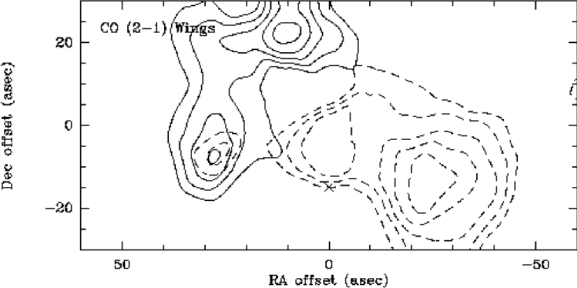
Figure 18: The SFO 20 CO ($J={2}\rightarrow{1}$) line wing emission. The blue lobe, indicated by dotted lines, is the integrated intensity in the range of 3 to 12 km s^-1. The red lobe, indicated by solid lines, is the integrated intensity in the range from 14 to 23 km s^-1. The lowest contour in each case is the half power contour. The x indicates the HCO⁺ ($J={3}\rightarrow{2}$) peak integrated intensity position.

Analysis of the HCO⁺ ($J={1}\rightarrow{0}$) centroid velocity, shown in Figure 17 indicates a small, but statistically significant gradient across the core. This gradient may indicate the cloud’s rotation. As an outflow has already been detected in this source by Sugitani et al. (1989) we chose to look at the CO ($J={2}\rightarrow{1}$) wing integrated intensity in order to try to verify the existing observation. Figure 18 shows that the line wings do show two lobes of emission, with the red lobe being predominantly northeast of the core and the blue lobe predominantly southwest of the core, similar to previous results. The cloud rotation shown in Figure 17 is perpendicular to the outflow, which is a prediction of current theories of star formation.

4.1.6 SFO 25

SFO 25, also known as HH124 (Walsh et al., 1992), is a type B cloud located at a distance of 780 pc. Embedded within is the IRAS source 06382+1017, whose spectral energy distribution is consistent with an embedded YSO . SFO 25 is associated with the HII region NGC 2264. Figure 2 shows a moderately curved rim arching northwards away from the ionizing source. However, although there is no tail visible in the optical, there is also no point at which the structure begins to broaden away from the ionizing source as there is for the other type B sources, SFO 4 and SFO 13. As we shall see below, this source bears many similarities with type C cometary clouds as well.

The CO ($J={1}\rightarrow{0}$) and CO ($J={2}\rightarrow{1}$) profiles show a wide (5 km s^-1), slightly asymmetric line (Figure 15b). The CO ($J={2}\rightarrow{1}$) profile shows line wings, which may indicate the presence of an outflow. The HCO⁺ line profiles show some asymmetry as well, mostly in the form of a redshifted tail.

The CO ($J={1}\rightarrow{0}$) integrated intensity map (Figure 19) shows a low level of CO emission throughout the region, which may be the result of contamination from nearby diffuse clouds which lie at nearly the same velocity of SFO 25. The C¹⁸O ($J={1}\rightarrow{0}$) traces the higher column density gas which forms the SFO 25 core and shows a molecular gas tail to the north. This morphology is more typical of a type C cometary cloud than a type B source. The CO ($J={2}\rightarrow{1}$) emission peaks strongly at the IRAS source position. The HCO⁺ ($J={1}\rightarrow{0}$) integrated intensity map (Figure 19) shows strongly peaked emission around the core with much weaker emission along the tail to the north of the source, which looks more typical of a type C source than a type B source. The HCO⁺ ($J={3}\rightarrow{2}$) emission is also strongly peaked at the IRAS source position.

We detected no coherent velocity structure in the HCO⁺ ($J={1}\rightarrow{0}$) velocity centroid observations. However the CO ($J={2}\rightarrow{1}$) line wings show evidence of an outflow oriented in the north-south direction (Figure 20), though unrelated emission near the same velocity makes it hard to separate the outflow emission from emission due to other sources.

4.1.7 SFO 37

SFO 37, also known as GN 21.38.9, is a type C cloud (SFO). It’s cometary structure is quite striking in the optical (Figure 2). SFO 37 is associated with the HII region IC1396 located at a distance of 750 pc. Embedded within is the IRAS source 21388+5622 whose spectral energy distribution is consistent with an embedded YSO. An investigation of this region by Duvert et al. (1990) revealed H$\alpha$ and [SII] emission on the northeast side of the molecular emission core. This emission is consistent with an ionization front driven by the strong UV field of a neighboring O6 star.

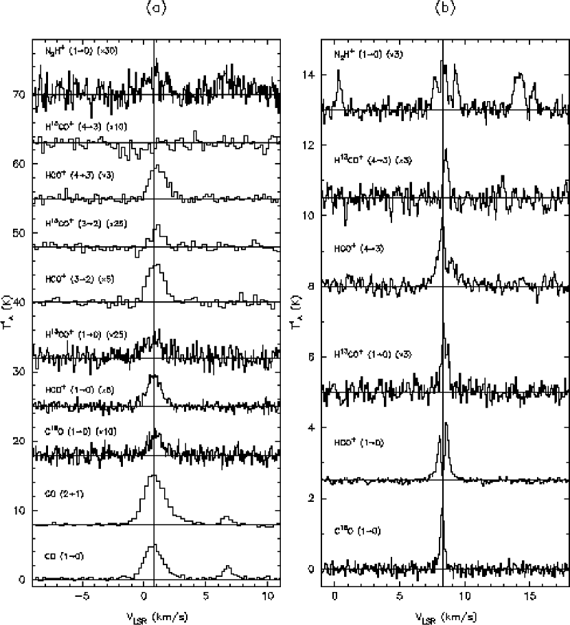
Figure 21: Line profiles of molecular transitions in the direction of the central IRAS source of SFO 37 (a) and B 335 (b).

The CO ($J={1}\rightarrow{0}$) and CO ($J={2}\rightarrow{1}$) line profiles (Figure 21a) shows a fairly gaussian shape centered at a line of sight velocity of approximately 1 km s^-1. A second component is visible at a line of sight velocity of approximately 7 km s^-1. Duvert et al. (1990) speculate that this second component may be a remnant of the low density gas shell in which the core formed, however we find this to be unlikely; the second component’s spatial distribution appears unrelated to that of the main component, and the low density gas surrounding the SFO 37 core has most likely been ionized. Both the HCO⁺ and H¹³CO⁺ profiles in Figure 21a appear fairly gaussian and share approximately the same centroid velocity. As is the case for many of these bright rimmed clouds, there is little or no indication of infall, despite the presence of a previously detected outflow (Duvert et al., 1990).

The integrated intensity map of the CO ($J={1}\rightarrow{0}$) emission shows the cometary cloud structure stretching from the center of the plot down to the southwest. There also appears to be a spur of gas 120^′′ south of the core extending west out of the tail of the cometary cloud (Figure 22). The CO ($J={2}\rightarrow{1}$) integrated intensity map also shows a cometary structure running northwest-southeast. Although we detected no outflow, the higher resolution survey of Duvert et al. (1990) detected a bipolar outflow with a 20^′′ separation between the red and blue lobes and a north-south orientation.

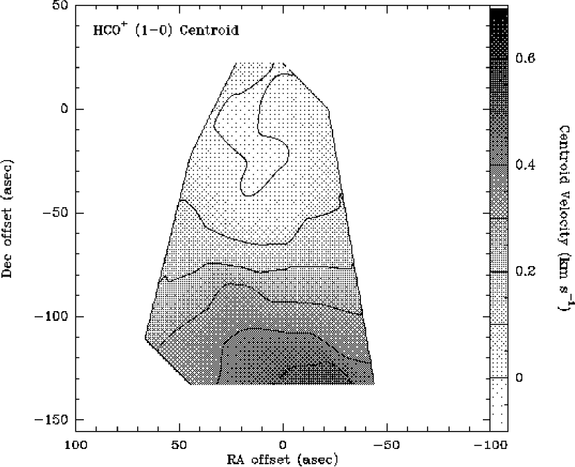
Figure 23: The SFO 37 centroid velocity integrated over the line core of HCO⁺ ($J={1}\rightarrow{0}$). The line of sight velocity has been subtracted out and the contours and greyscale are indicated on the wedge to the right of the figure.

The HCO⁺ ($J={1}\rightarrow{0}$) integrated intensity map (Figure 22) shows emission from the IRAS core, as well as an extension to the southeast. There is a centroid velocity gradient of the HCO⁺ ($J={1}\rightarrow{0}$) emission along the length of the cometary cloud (Figure 23). This velocity gradient may be due to the interaction of the ionization front and the cometary cloud. Recent near-infrared observations of this source have also shown several point sources which may be pre-main-sequence stars which lie on a line extending from the embedded IRAS source in the opposite direction as the tail (Sugitani et al., 1995, 1999). These young stars, and their extremely regular arrangement along the line which bisects the ionization front, which would be the line along which the dense core would travel in a radiation driven cometary globule (Lefloch & Lazareff, 1994), make this source an excellent candidate for small scale sequential star formation (Sugitani et al., 1999). The HCO⁺ ($J={1}\rightarrow{0}$) map shows evidence of some fragmentation of the tail of the cometary cloud into what could potentially seed the cores of new sequentially driven star formation. The HCO⁺ ($J={3}\rightarrow{2}$) and HCO⁺ ($J={4}\rightarrow{3}$) integrated intensity maps pick up the dense gas surrounding the central IRAS source. The second core, located approximately 100^′′ behind the IRAS source, has a lower excitation temperature than the core surrounding the IRAS source, which may indicate that it is much less dense. Once the ionization front moves past the IRAS source, it could continue on to this second core, inducing star formation once again. The IRAS source would become another young star in the line of young stars which originated in this sequential star forming region.

4.2 Bok Globules

4.2.1 B335

The dark cloud B335 has been well studied. The embedded IRAS source 19345+0727 appears to be a protostellar core which is the source of a bipolar outflow which is oriented in the east-west direction on the plane of the sky. The central source shows an elongation in the far-infrared and submillimeter continuum in the north-south direction, orthogonal to the outflow (Chandler et al., 1990). The high visual extinction and lack of near-infrared emission (Chandler & Sargent, 1993; Anglada et al., 1992) indicates that it may be a class 0 source. Zhou et al. (1993) provide evidence for protostellar collapse in B335 using H₂CO and CS observations. Subsequently, Zhou (1995) improved upon the infall models for B335 by including rotation and confirmed the earlier suggestion of infall. B335 is one of the best studied infall candidates, which is why we chose to observe it and compare it with the bright rimmed clouds.

The B335 line profiles (Figure 21b) are very narrow compared to the other sources we’ve observed. The optically thin lines show a velocity width of only about 1 km s^-1. This comparably narrow line width is more typical of nearby isolated star forming regions than the large line widths we see in the bright rimmed clouds. This is probably due to the fact that bright rimmed clouds are on average more distant and larger than many of the Bok globules observed in millimeter and submillimeter wavelengths. As a result of the relationship between cloud size and velocity dispersion (Larson, 1981; Myers & Goodman, 1988) we expect the bright rimmed clouds to have generally larger line widths than smaller clouds such as B335 or CB 224.

The HCO⁺ ($J={1}\rightarrow{0}$) profile shows a large self-absorption trough, however the centroid is not blue shifted, as one would expect for infall, but red-shifted. This is a result of the core rotation (Zhou, 1995) and the large beam of FCRAO. The HCO⁺ ($J={4}\rightarrow{3}$) line profile also shows self absorption, which results in a double-peaked spectrum. This spectrum, however, shows a considerable blue-shifted centroid relative to its isotopic counterpart. The H¹³CO⁺ ($J={1}\rightarrow{0}$) and H¹³CO⁺ ($J={4}\rightarrow{3}$) show single peaks right at the point where the HCO⁺ lines are most self-absorbed, indicating that there is a high optical depth of HCO⁺ at those velocities, and not that there are two different molecular cloud structures with slightly differing velocities in that direction.

The C¹⁸O ($J={1}\rightarrow{0}$) and N₂H⁺ ($J={1}\rightarrow{0}$) emission is confined to the core, which does not seem to be resolved by our beam (Figure 24). The HCO⁺ ($J={1}\rightarrow{0}$) emission is resolved by the FCRAO beam, and seems to peak at the position of the IRAS core. The HCO⁺ ($J={1}\rightarrow{0}$) centroid map (Figure 25) does not indicate any coherent structure across the cloud. The HCO⁺ ($J={4}\rightarrow{3}$) emission is elongated in the east-west direction, along the outflow (Figure 24). The centroid velocity of HCO⁺ ($J={4}\rightarrow{3}$) has a coherent gradient running north-south indicating that B335 may be rotating around the axis defined by its outflow (Narayanan, 1997).

4.2.2 CB 3

CB 3 (Clemens & Barvainis, 1988), also known as L 594 (Lynds, 1965), is a Bok globule located approximately 2500 pc from us (Launhardt & Henning, 1997). Embedded within it is the IRAS source 00259+5625, which has an extremely high luminosity (930 $L_{\sun}$) and appears to be a source of isolated intermediate- or high- mass star formation, not typically associated with Bok globules (see Codella & Bachiller (1999) and references therein). Because this source is so distant and has such a high luminosity IRAS source it is not typically studied as a source of low-mass star formation, but it may be a good counterpart for the more distant bright rimmed clouds, such as SFO 13, SFO 25, or SFO 37.

The CB 3 CO central line profiles (Figure 26a) are more complex than many of the bright rimmed cloud’s line profiles. Both the CO ($J={1}\rightarrow{0}$) and CO ($J={2}\rightarrow{1}$) profiles show a component near the N₂H⁺ line center velocity, and a second component red shifted by a couple of km s^-1 from the first. The C¹⁸O ($J={1}\rightarrow{0}$) line does not show two components, but does have a significant red shifted tail. The HCO⁺ ($J={1}\rightarrow{0}$) central line profile is blue-shifted relative to both the N₂H⁺ ($J={1}\rightarrow{0}$) line as well as the H¹³CO⁺ ($J={1}\rightarrow{0}$) line, which could indicate infall in the core. The HCO⁺ ($J={3}\rightarrow{2}$) line shows less self-absorption on the red-shifted side of the line, but still has a centroid velocity which is slightly blue relative to the N₂H⁺ profile.

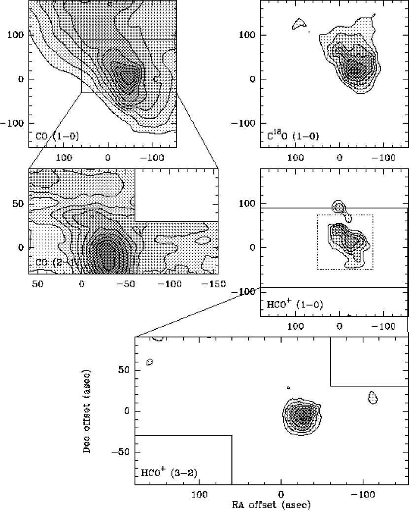
Figure 27: Integrated intensity maps of CB 3 in various transitions and isotopomers of HCO⁺and CO. The IRAS source 00259+5625 is located at the center of each map. The CO ($J={1}\rightarrow{0}$) map has a lowest contour of 2.2 K km s^-1 ($3\sigma$) and increments of 2.2 K km s^-1 ($3\sigma$). The CO ($J={2}\rightarrow{1}$) map has a lowest contour of 3.1 K km s^-1 ($3\sigma$) and increments of 5.1 K km s^-1 ($5\sigma$). The C¹⁸O ($J={1}\rightarrow{0}$) map has a lowest contour of 0.5 K km s^-1 ($3\sigma$) and increments of 0.2 K km s^-1 ($1\sigma$). The HCO⁺ ($J={1}\rightarrow{0}$) map has a lowest contour of 0.5 K km s^-1 ($3\sigma$) and increments of 0.2 K km s^-1 ($1\sigma$). The HCO⁺ ($J={3}\rightarrow{2}$) map has a lowest contour of 1.5 K km s^-1 ($3\sigma$) and increments of 0.5 K km s^-1 ($3\sigma$). The dotted rectangle in the HCO⁺ ($J={1}\rightarrow{0}$) map indicates the region over which the HCO⁺ centroid is shown in figure 28.

The CO ($J={1}\rightarrow{0}$) integrated intensity map (Figure 27) shows a ridge of gas running northeast–southwest, but no peak at the core, however the CO ($J={2}\rightarrow{1}$) map clearly shows the core, which is displaced from the (0,0) position, but remains consistent with the error position of the IRAS source. The C¹⁸O ($J={1}\rightarrow{0}$) also highlights the position of the dense core along the low-density molecular gas ridge. The HCO⁺ ($J={1}\rightarrow{0}$) integrated intensity map shows the gas core, with some extension along the ridge, however the HCO⁺ ($J={3}\rightarrow{2}$) emission is centered only on the core position.

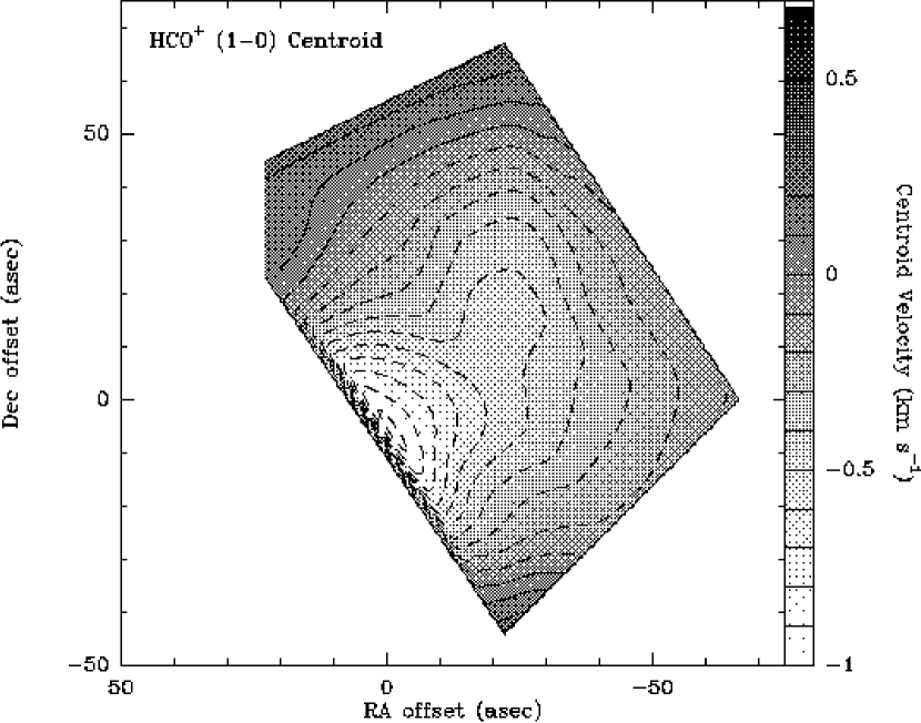
Figure 28: The CB 3 centroid velocity integrated over the line core of HCO⁺ ($J={1}\rightarrow{0}$). The line of sight velocity has been subtracted out and the contours and greyscale are indicated on the wedge to the right of the figure.

The HCO⁺ ($J={1}\rightarrow{0}$) emission does not show a linear velocity gradient, but does have some structure (Figure 28). The CO ($J={2}\rightarrow{1}$) line wing map (Figure 29) shows a bipolar structure with the blue-shifted line wing to the south of the core and the red-shifted wing to the north. This indicates the probable presence of a bipolar outflow in this core. Our detection of this outflow is consistent with the outflow detected by Codella & Bachiller (1999).

4.2.3 CB 224

CB 224 (Clemens & Barvainis, 1988) is a Bok globule located at a distance of approximately 450 pc, and it’s embedded IRAS source, 20355+6343, has a luminosity of 3.9 $L_{\sun}$ (Launhardt & Henning, 1997). This is very comparable to many of the SFO sources discussed above, making CB 224 a good isolated source to compare with the potentially triggered SFO sources. CB 224, however, has very weak molecular emission lines.

The CO ($J={1}\rightarrow{0}$) central line profile shows evidence of a blue-shifted wing, which is not present in the C¹⁸O ($J={1}\rightarrow{0}$) profile. This may indicate the presence of an outflow (Figure 26b). The HCO⁺ ($J={1}\rightarrow{0}$) line profile is blue-shifted relative to both the N₂H⁺ emission, and the H¹³CO⁺ ($J={1}\rightarrow{0}$) emission profile. The HCO⁺ ($J={1}\rightarrow{0}$) profile shows a knee right where the H¹³CO⁺ emission peaks indicating a fairly classical self-absorption profile typical of infall regions. The HCO⁺ ($J={3}\rightarrow{2}$) profile shows some evidence of a slight centroid blue-shift relative to the H¹³CO⁺ ($J={3}\rightarrow{2}$) line and the N₂H⁺ ($J={1}\rightarrow{0}$) line, but it is not as convincing an infall signature as the lower energy transition.

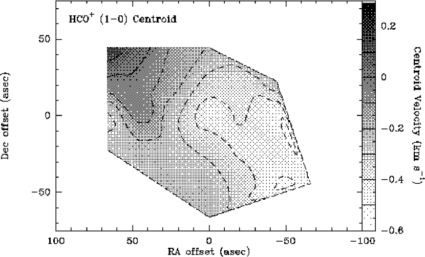
Figure 31: The CB 224 centroid velocity integrated over the line core of HCO⁺ ($J={1}\rightarrow{0}$). The line of sight velocity has been subtracted out and the contours and greyscale are indicated on the wedge to the right of the figure.

The CO ($J={1}\rightarrow{0}$) integrated intensity map shows molecular emission is fairly ubiquitous around this source (Figure 30), however there are two CO peaks, one north and one south of the IRAS core. The HCO⁺ ($J={1}\rightarrow{0}$) integrated intensity map clearly highlights the core gas surrounding the IRAS source at the center of the map. There is a gradient running northeast–southwest in the HCO⁺ ($J={1}\rightarrow{0}$) centroid velocity which could indicate rotation in the core (Figure 31).

5 Discussion

5.1 Core Masses

Of the seven bright rimmed clouds observed and the three Bok globules, all the sources show evidence of a very dense core with the exception of SFO 4, which is unusual in that it appears to be a fairly diffuse cloud. Turner (1995) has shown that the N₂H⁺ ($J={1}\rightarrow{0}$) transition can be a good probe of the properties of star forming cores. While CO, HCO⁺, and other molecules have a tendency to freeze on to grains in the low temperature, high density environment of cores, N₂H⁺ remains relatively undepleted (Bergin & Langer, 1997) in dark cloud cores, making it a good probe of the density profile. N₂H⁺ ($J={1}\rightarrow{0}$) also has several fine structure lines (Caselli et al., 1995) which can be used to derive the excitation temperature of the N₂H⁺ ($J={1}\rightarrow{0}$) line. We use the “hyperfine structure (hfs) method” in CLASS (Forveille et al., 1989) to derive these properties from the N₂H⁺ emission, using the component separations observed by Caselli et al. (1995). The excitation temperature and the optical depth derived from the hyperfine line ratios can be used to derive the column density of gas within the telescope beam, which can be related to the gas mass in the beam, assuming a relative abundance ratio between N₂H⁺ and molecular hydrogen (Benson et al., 1998). We have performed this analysis for the objects in our sample, and the results are shown in Table 3. The column densities of N₂H⁺ fall within the same range of column densities observed in the cores of dark clouds (Benson et al., 1998).

The mass of the core can also be derived by comparing the emission of HCO⁺ ($J={1}\rightarrow{0}$) to H¹³CO⁺ ($J={1}\rightarrow{0}$), under the assumption that the H¹³CO⁺ emission is optically thin. The optical depth can be derived from assuming an abundance ratio between the C and ¹³C isotopes, and comparing the ratio of H¹³CO⁺ emission to HCO⁺ emission. Then the excitation temperature is derived by assuming a filling factor of unity, and the excitation temperature and optical depth are used to derive the column density of gas. The results of this analysis are presented in table 4. It is encouraging to see that even though N₂H⁺ and HCO⁺ do not trace exactly the same gas they produce fairly comparable results for the overall core mass. These clouds tend to have cores with masses on the order of tens of solar masses.

5.2 Outflows

Outflows appear to be fairly ubiquitous in our sample. We detected outflows in nearly all the sources we surveyed. This is to be expected, since a star is forming and the cloud must dissipate its angular momentum in order to collapse. However, in the case of shock triggered regions, the ionization front does dissipate some of the angular momentum of the collapsing cloud (Elmegreen, 1992), though the ionization front would probably not have a noticeable effect on the scale of the accretion disk.

We have analyzed the energy in the detected outflows and present the results in table 5. We derived the mass of the lobes by averaging the integrated intensity of the line-wing emission over the spatial extend of the lobe. We then derived a column density from this integrated intensity assuming that the emission is optically thin and an excitation temperature of 30K. The momentum ($P$) and kinetic energy (KE) of an outflow can be derived by computing

$$P=\sum_{\rm ch}m_{\rm ch}v_{\rm ch},\ {\rm and}\ {\rm KE}=\frac{1}{2}\sum_{\rm ch}m_{\rm ch}v_{\rm ch}^{2}$$

along the spatially averaged spectrum of the outflow lobe. Unless the outflow is along the line of sight, this method underestimates these quantities by a factor of $\sin(i)$ where $i$ is the inclination of the outflow relative to the plane of the sky. As this method tends to underestimate the momentum and kinetic energy of the outflow, and since these estimates have fairly large uncertainties we chose not to integrate over the averaged spectrum, but instead to calculate the momentum to be $M_{\rm total}V_{\rm max}$ and kinetic energy to be $\frac{1}{2}M_{\rm total}V_{\rm max}^{2}$ where $M_{\rm total}$ is the total mass of the outflow lobe, and $V_{\rm max}$ is the maximum measured velocity of the outflow lobe relative to the line center. This assumes that all the material in the flow is moving at the maximum observed velocity, and that the lower velocities are the result of projection effects. This technique results in upper limit estimates of the flow’s momentum and energy (Walker et al., 1988). The dynamical age ($\tau_{d}$) of the flow is found by calculating the distance from the core to the edge of the outflow lobe and dividing by $V_{\rm max}$, while the kinetic luminosity ($L$) is derived by deviding the kinetic energy of the lobe by the dynamical age of the flow.

The dynamical ages and kinetic luminosities of these outflows tend to agree with those of previously observed outflow sources (Saraceno et al., 1996). The outflow ages all tend to be greater than $10^{4}$ years, which may indicate that the embedded objects are class I sources rather than class 0 sources, which typically have outflow ages less than $10^{4}$ years (Saraceno et al., 1996).

We compare the mechanical luminosity and force needed to accelerate the outflow to the luminosity and radiant pressure of the IRAS source driving the outflow in Figure 32. We find that the bright rimmed clouds occupy similar regions in the two plots indicating that they are probably driven by similar processes as the other outflows around forming stars that have been observed to date. We find that the embedded IRAS source has sufficient energy to drive the outflows we observe, but that the radiant pressure of the IRAS source is not sufficient to accelerate the outflows to the velocities we observe. This confirms similar observations of Lada (1985).

5.3 Infall Motion

Although several outflows were detected, and the presence of outflows implies infalling gas, there were few line asymmetries indicative of infall in the bright rimmed clouds. Mardones et al. (1997) have defined a parameter to quantify the line asymmetry in terms of the line center velocity of an optically thick line, the line center velocity of an optically thin line, and the width of the optically thin line. The asymmetry ($\delta V$) is then defined as

$$\delta V=\left(V_{\rm thick}-V_{\rm thin}\right)/\Delta V_{\rm thin}.$$

Mardones et al. (1997) find the line center velocities of both the thick and thin lines by fitting a gaussian to the lines, however this does not yield a very robust estimator of the asymmetry in my opinion. As the optical depth increases, the thick line does immediately separate into two distinguishable components. At moderate optical depths a knee forms in the line profile as the peak becomes blue-shifted. A gaussian fit to this type of profile is very inaccurate, however the centroid of this profile is well determined. Therefore we use the centroid velocity of the thick line when calculating the line asymmetry.

We tabulate our line asymmetry values in table 6. The millimeter asymmetry is derived from observations of the HCO⁺ ($J={1}\rightarrow{0}$) optically thick line and the H¹³CO⁺ ($J={1}\rightarrow{0}$) optically thin line. The submillimeter asymmetry value is derived from the observations of the HCO⁺ ($J={3}\rightarrow{2}$) optically thick line and the H¹³CO⁺ ($J={3}\rightarrow{2}$) optically thin line. Mardones et al. (1997) suggest that a $\delta V$ between –0.25 and 0.25 be considered symmetric. All the bright rimmed clouds, with the exception of SFO 18, show no significant asymmetry in their central line profiles according to this criterion.

Previous studies of class 0 and class I sources performed using the millimeter CS ($J={2}\rightarrow{1}$) transition (Mardones et al., 1997) and the submillimter HCO⁺ ($J={3}\rightarrow{2}$) transition (Gregersen et al., 2000) show preferentially blue asymmetric line profiles, thought to be the result of infall in these star forming cores. Mardones et al. (1997) quantify the overall predilection of the observed sources to have blue asymmetric line profiles in terms of a parameter they call the “blue excess” which is defines as

$$\mbox{blue excess}=\frac{N_{\rm blue}-N_{\rm red}}{N_{\rm total}}.$$

where $N_{\rm blue}$ is the number of sources with $\delta V<-0.25$, $N_{\rm red}$ is the number of sources with $\delta V>0.25$, and $N_{\rm total}$ is the total number of sources. Gregersen et al. (2000) find a blue excess of 0.28 for the class 0 and class I sources they observe, and an overall blue excess of 0.31 for all the sources in the literature. The bright rimmed clouds have a blue excess of 0.2 measured in both the millimeter and submillimeter transitions, however that is measured with a sample of only 6 sources. A scatter plot, comparing the asymmetry of the bright rimmed clouds and Bok globules we observed with those observed by Mardones et al. (1997) and Gregersen et al. (2000) is shown in Figure 33. We see that the bright rimmed clouds show asymmetry values comparable to those of other star forming regions. The bright rimmed clouds, however, do not show as wide a deviation of asymmetry values, and tend to have $\delta V$s which are closer to 0 than typical star formation regions, whose $\delta V$s tend to be negative. A wider survey of bright rimmed clouds is required to determine if they indeed have significantly less blue excess than other YSOs.

Why do we not detect infall in more bright rimmed clouds? Does the incoming shock front produce conditions that alter the shape of the emergent line profile? An isolated Bok globule usually has an excitation temperature profile which drops from a value on the order of 20–50K at the core center to 10K at the edge of the core. Bright rimmed clouds, however, are stripped of their molecular envelopes and heated by UV flux from O stars. This may be expected to flatten or in some cases invert the temperature profile, so that the cloud core center may still have a physical temperature around 20K, but the edge of the cloud core may have a physical temperature of several hundred K. Since the gas throughout the core is fairly excited, it would eliminate the self-absorption which characterizes the blue line asymmetry typically associated with infall. This inversion of the excitation temperature gradient could even lead to absorption of the blue-shifted gas by denser, yet less excited gas closer to the core. Figure 34 illustrates the effect of inverting the temperature gradient on a free-falling infall region. The model presented in that figure is a collapsing region, with a peak density of $10^{7}$ cm^-3 which drops down to a density of $10^{4}$ cm^-3 near the edge of the beam. The infall region is confined to an area which is roughly 50% of the beam size. We assume a free-fall collapse models, with infall velocities increasing towards the center of the collapsing sphere. The only difference between the model which generates the double peaked solid line and the single peaked dashed line is the temperature gradient across the infalling region. The solid line is the result of a linear temperature gradient which peaks in the center at 40 K and drops off towards the edge of our beam to 10 K. The dashed line also is a linear temperature gradient, but the temperature increases from 40 K at the center of the sphere to 300 K at the outer edge. The approximates more closely the behavior of infalling gas clouds under the influence of wind-triggered collapse as modeled by VC. Our model shows that heating of the envelope of a collapsing cloud can lessen or remove entirely the blue-asymmetric line signature of a collapsing molecular cloud.

In order to test the assumption that the ionization front may be raising the excitation temperature near the edge of the cloud, we have smoothed the HCO⁺ ($J={3}\rightarrow{2}$) map to the same resolution as the HCO⁺ ($J={1}\rightarrow{0}$) in both a bright rimmed cloud (SFO 25) and a Bok globule (CB 3) which we observed. We assume thermodynamic equilibrium between these transitions, as well as a low optical depth in order to derive the excitation temperature across the core. SFO 25 has fairly gaussian lines, centered at the same velocity as their isotopic counterparts, indicating that the HCO⁺ emission for this source may be optically thin. In CB 3, as in all the Bok globules we observed, we know the HCO⁺ emission is not optically thin, however this would tend to wash out the excitation temperature to the cloud core, so in regions where the emission is optically thick we can consider the derived excitation temperature to be a lower limit. Towards the edge of the CB 3 core the HCO⁺ emission does become optically thin making this a good assumption. In the case of SFO 25 we derive the excitation temperature along a line which cuts through both the ionization front and the star forming core, and plot that excitation temperature profile in Figure 35a. The center (0^′′) offset represents the star forming core position, and the ionization front is in the negative direction. Figure 35b shows the excitation temperature profile around the core of CB 3, however we averaged annuli around the central core in order to derive the plotted values, rather than take a cut straight across in order to maximize our signal to noise ratio. In the case of SFO 25, the excitation temperature peaks near the edge of the cloud core, while in CB 3 the excitation temperature peaks near the center. Although it is likely that the cores of these bright rimmed clouds are collapsing in a similar manner to other class 0 or class I sources, the heating due to the nearby HII region may dampen their spectral line infall signature.

6 Conclusions

Our observations constitute the first detailed millimeter and submillimeter multitransition study of bright rimmed clouds. Among the 7 bright rimmed clouds we observe, 6 seem to share traits similar with other low to intermediate mass star forming regions. Our analysis of these bright rimmed clouds has yielded the principal results that follow.

1. New FCRAO CO ($J={1}\rightarrow{0}$), C¹⁸O ($J={1}\rightarrow{0}$), HCO⁺ ($J={1}\rightarrow{0}$), H¹³CO⁺ ($J={1}\rightarrow{0}$), and N₂H⁺ ($J={1}\rightarrow{0}$) observations along with new HHT CO ($J={2}\rightarrow{1}$), HCO⁺ ($J={3}\rightarrow{2}$), HCO⁺ ($J={4}\rightarrow{3}$), H¹³CO⁺ ($J={3}\rightarrow{2}$), and H¹³CO⁺ ($J={4}\rightarrow{3}$) observations of 7 bright rimmed clouds and 3 Bok globules were presented. These observations constitute the most detailed millimeter and submillimeter study of bright rimmed clouds to date.

2. The millimeter CO and HCO⁺ emission tends to terminate abruptly at the ionization front. As a result, the overall morphology of the CO and HCO⁺ millimeter integrated intensity maps are similar with the optical morphologies identified by SFO.

3. The millimeter HCO⁺ tends to show the dense swept up ridge behind the ionization front, as well as the star forming core around the embedded IRAS source. In some of the bright rimmed clouds the HCO⁺ ($J={1}\rightarrow{0}$) emission also traces other overdense clumps which may later be triggered to collapse by the ionization front, resulting in sequential star formation.

4. The millimeter and submillimeter HCO⁺ lines from many of the bright rimmed clouds appear nearly gaussian, with little evidence of infall asymmetry. The only exceptions to this are SFO 18, which shows significant blue asymmetry, and SFO 16 which shows a slight red asymmetry relative to optically thin tracers.

5. The core masses derived for the bright rimmed clouds using both N₂H⁺ and HCO⁺ are typical for low and intermediate mass star formation regions. The N₂H⁺ and HCO⁺ results also tend to agree to within an order of magnitude.

6. The overall blue excess of the sample of bright rimmed clouds is slightly less than that of the class 0 and class I sources observed by Mardones et al. (1997) and Gregersen et al. (2000), though the small number of bright rimmed clouds we observed does not make this difference statistically significant. A larger survey of bright rimmed clouds is required to determine if this is a significant finding. We do however make a case for the fact that the heating of the collapsing cloud by the adjacent HII region could dampen the infall signature, lowering the blue excess of bright rimmed clouds.

7. We observed outflows around 5 of the 7 bright rimmed clouds, including new detections of outflows around SFO 13 and SFO 25. These outflows appear to have similar properties to other outflows detected in millimeter and submillimeter emission.

We do not see direct evidence of triggering in these sources. We can not determine if star formation was induced in these clouds or if we are seeing the collapse of pre-existing clumps. We do know that the environment has a profound effect on these regions. Although we have found similarities and differences between Bok globules and bright rimmed clouds, a detailed understanding of the effects of an ionization front on star formation can only be achieved by theoretically modeling this process, and then comparing that model to observations. In a forthcoming paper we will compare these observations with models of shock driven collapse derived by VC. In addition to bright rimmed clouds, these models could explain the effect of outflows and other environmental effects on star formation. Development of the techniques and models which will help us understand star formation in complex environments is in progress.

We gratefully acknowledge the staff of the HHT for their excellent support. In particular we wish to thank Harold Butner for his assistance with setting up our OTF observations at the HHT and Mark Heyer for his many helpful comments. C. H. De Vries and G. Narayanan are supported by the FCRAO under the National Science Foundation grant AST 01-00793.

Figure 1: This schematic shows a planar shock from approaching a dense clump (0). As the shock front hits the clump it slows down, and the clump flattens out, this corresponds to the type A morphology. The clump contracts under the influence of the shock front, and shields the gas behind it from ionization as the shock front passes, this corresponds to the type B morphology. The clump continues to contract and shield the gas behind it, forming a cometary morphology, this correspondes to the type C morphology.

Figure 3: Line profiles of molecular transitions in the direction of the central IRAS source of SFO 4 (a) and SFO 13 (b).

Figure 7: The SFO 13 CO ($J={2}\rightarrow{1}$) line wing emission. The blue lobe, indicated by dotted lines, is the integrated intensity in the range of –48 to –39.5 km s^-1. The red lobe, indicated by solid lines, is the integrated intensity in the range from –37.5 to –28 km s^-1. The lowest contour in each case is the half power contour. The x indicates the HCO⁺ ($J={3}\rightarrow{2}$) peak integrated intensity position.

Figure 10: The SFO 16 centroid velocity integrated over the line core of HCO⁺ ($J={1}\rightarrow{0}$). The line of sight velocity has been subtracted out and the contours and greyscale are indicated on the wedge to the right of the figure.

Figure 11: The SFO 16 CO ($J={2}\rightarrow{1}$) line wing emission. The blue lobe, indicated by dotted lines, is the integrated intensity in the range of –2 to 7.2 km s^-1. The red lobe, indicated by solid lines, is the integrated intensity in the range from 9 to 18 km s^-1. The lowest contour in each case is the half power contour. The x indicates the HCO⁺ ($J={3}\rightarrow{2}$) peak integrated intensity position.

Figure 14: The SFO 18 CO ($J={1}\rightarrow{0}$) line wing emission. The blue lobe, indicated by dotted lines, is the integrated intensity in the range of 2 to 11 km s^-1. The red lobe, indicated by solid lines, is the integrated intensity in the range from 13 to 22 km s^-1. The lowest contour in each case is the half power contour. The x indicates the C¹⁸O ($J={1}\rightarrow{0}$) peak integrated intensity position.

Figure 16: Integrated intensity maps of SFO 20 in various transitions and isotopomers of HCO⁺and CO. The IRAS source 05173–0555 is located at the center of each map. The CO ($J={1}\rightarrow{0}$) map has a lowest contour of 1.1 K km s^-1 ($3\sigma$) and increments of 1.1 K km s^-1 ($3\sigma$). The CO ($J={2}\rightarrow{1}$) map has a lowest contour of 1.0 K km s^-1 ($3\sigma$) and increments of 3.4 K km s^-1 ($10\sigma$). The C¹⁸O ($J={1}\rightarrow{0}$) map has a lowest contour of 0.4 K km s^-1 ($3\sigma$) and increments of 0.1 K km s^-1 ($1\sigma$). The HCO⁺ ($J={1}\rightarrow{0}$) map has a lowest contour of 0.4 K km s^-1 ($3\sigma$) and increments of 0.1 K km s^-1 ($1\sigma$). The HCO⁺ ($J={3}\rightarrow{2}$) map has a lowest contour of 0.6 K km s^-1 ($3\sigma$) and increments of 0.2 K km s^-1 ($1\sigma$). The dotted rectangle in the HCO⁺ ($J={1}\rightarrow{0}$) map indicates the region over which the HCO⁺ centroid is shown in figure 17.

Figure 17: The SFO 20 centroid velocity integrated over the line core of HCO⁺ ($J={1}\rightarrow{0}$). The line of sight velocity has been subtracted out and the contours and greyscale are indicated on the wedge to the right of the figure.

Figure 19: Integrated intensity maps of SFO 25 in various transitions and isotopomers of HCO⁺and CO. The IRAS source 06382+1017 is located at the center of each map. The CO ($J={1}\rightarrow{0}$) map has a lowest contour of 3.6 K km s^-1 ($3\sigma$) and increments of 6.1 K km s^-1 ($5\sigma$). The CO ($J={2}\rightarrow{1}$) map has a lowest contour of 1.7 K km s^-1 ($3\sigma$) and increments of 5.6 K km s^-1 ($10\sigma$). The C¹⁸O ($J={1}\rightarrow{0}$) map has a lowest contour of 0.5 K km s^-1 ($3\sigma$) and increments of 0.4 K km s^-1 ($2\sigma$). The HCO⁺ ($J={1}\rightarrow{0}$) map has a lowest contour of 0.5 K km s^-1 ($3\sigma$) and increments of 0.8 K km s^-1 ($5\sigma$). The HCO⁺ ($J={3}\rightarrow{2}$) map has a lowest contour of 1.2 K km s^-1 ($3\sigma$) and increments of 2.0 K km s^-1 ($5\sigma$). The dashed contour in the HCO⁺ ($J={3}\rightarrow{2}$) indicates the half power contour of the N₂H⁺ ($J={1}\rightarrow{0}$) emission.

Figure 20: The SFO 25 CO ($J={2}\rightarrow{1}$) line wing emission. The blue lobe, indicated by dotted lines, is the integrated intensity in the range of –2 to –5.5 km s^-1. The red lobe, indicated by solid lines, is the integrated intensity in the range from 9 to 18 km s^-1. The lowest contour in each case is the half power contour. The x indicates the HCO⁺ ($J={3}\rightarrow{2}$) peak integrated intensity position.

Figure 22: Integrated intensity maps of SFO 37 in various transitions and isotopomers of HCO⁺and CO. The IRAS source 21388+5622 is located at the center of each map. The CO ($J={1}\rightarrow{0}$) map has a lowest contour of 1.4 K km s^-1 ($3\sigma$) and increments of 1.4 K km s^-1 ($3\sigma$). The CO ($J={2}\rightarrow{1}$) map has a lowest contour of 1.6 K km s^-1 ($3\sigma$) and increments of 2.6 K km s^-1 ($5\sigma$). The HCO⁺ ($J={1}\rightarrow{0}$) map has a lowest contour of 0.4 K km s^-1 ($3\sigma$) and increments of 0.2 K km s^-1 ($1\sigma$). The HCO⁺ ($J={3}\rightarrow{2}$) map has a lowest contour of 0.8 K km s^-1 ($3\sigma$) and increments of 0.3 K km s^-1 ($1\sigma$). The HCO⁺ ($J={4}\rightarrow{3}$) map has a lowest contour of 0.9 K km s^-1 ($3\sigma$) and increments of 0.3 K km s^-1 ($1\sigma$). The dotted rectangle in the HCO⁺ ($J={1}\rightarrow{0}$) map indicates the region over which the HCO⁺ centroid is shown in figure 23.

Figure 24: Integrated intensity maps of B335 in various transitions and isotopomers of HCO⁺and CO. The IRAS source 19345+0727 is located at the center of each map. The C¹⁸O ($J={1}\rightarrow{0}$) map has a lowest contour of 0.6 K km s^-1 ($3\sigma$) and increments of 0.2 K km s^-1 ($1\sigma$). The HCO⁺ ($J={1}\rightarrow{0}$) map has a lowest contour of 0.3 K km s^-1 ($3\sigma$) and increments of 0.1 K km s^-1 ($1\sigma$). The HCO⁺ ($J={4}\rightarrow{3}$) map has a lowest contour of 0.8 K km s^-1 ($3\sigma$) and increments of 0.3 K km s^-1 ($1\sigma$). The dotted rectangle in the HCO⁺ ($J={1}\rightarrow{0}$) map indicates the region over which the HCO⁺ centroid is shown in figure 25. The dashed contour in the C¹⁸O ($J={1}\rightarrow{0}$) indicates the half power contour of the N₂H⁺ ($J={1}\rightarrow{0}$) emission.

Figure 25: The B335 centroid velocity integrated over the line core of HCO⁺ ($J={1}\rightarrow{0}$). The line of sight velocity has been subtracted out and the contours and greyscale are indicated on the wedge to the right of the figure.

Figure 26: Line profiles of molecular transitions in the direction of the central IRAS source of CB 3 (a) and CB 224 (b).

Figure 29: The CB 3 CO ($J={2}\rightarrow{1}$) line wing emission. The blue lobe, indicated by dotted lines, is the integrated intensity in the range of –49 to –39.5 km s^-1. The red lobe, indicated by solid lines, is the integrated intensity in the range from –37 to –29 km s^-1. The lowest contour in each case is the half power contour. The x indicates the HCO⁺ ($J={3}\rightarrow{2}$) peak integrated intensity position.

Figure 30: Integrated intensity maps of CB 224 in various transitions and isotopomers or HCO⁺and CO. The IRAS source 20355+6343 is located at the center of each map. The CO ($J={1}\rightarrow{0}$) map has a lowest contour of 2.4 K km s^-1 ($3\sigma$) and increments of 0.8 K km s^-1 ($1\sigma$). The HCO⁺ ($J={1}\rightarrow{0}$) map has a lowest contour of 0.3 K km s^-1 ($3\sigma$) and increments of 0.1 K km s^-1 ($1\sigma$). The dotted rectangle in the HCO⁺ ($J={1}\rightarrow{0}$) map indicates the region over which the HCO⁺ centroid is shown in figure 31. The dashed contour in the HCO⁺ ($J={1}\rightarrow{0}$) indicates the half power contour of the N₂H⁺ ($J={1}\rightarrow{0}$) emission.

Figure 32: The energetics of the outflow are compared with those of the photons arising from the embedded IRAS sources we observed. The open squares represent the bright rimmed clouds we observed, the open circle is CB 3 and the closed circles are data from Lada (1985). Figure (a) shows the outflow mechanical luminosity compared to the luminosity of the IRAS source. Figure (b) compares the force needed to accelerate the molecular outflows to the total radiant pressure of the central object. The dashed lines indicate where forces or luminosities are equal. The bright rimmed clouds share similar properties with previously observed outflows, namely that although there exists enough energy in the central source to drive the outflows, radiative scattering is not the source of the outflow’s acceleration.

Figure 33: The line asymmetry parameter ($\delta V$) towards the star forming core measured in both millimeter (x–axis) and submillimeter (y–axis) molecular transitions. The open triangles are the bright rimmed clouds reviewed in this paper observed in the millimeter transition HCO⁺ ($J={1}\rightarrow{0}$) and the submillimeter transition HCO⁺ ($J={3}\rightarrow{2}$). The filled triangles are the Bok globules we observed in the same transitions as the bright rimmed clouds. The filled circles are class I and class 0 sources observed in the millimeter CS ($J={2}\rightarrow{1}$) transition by Mardones et al. (1997) and in the submillimeter HCO⁺ ($J={3}\rightarrow{2}$) transition by Gregersen et al. (2000).

Figure 34: The blue-asymmetric line profile is very dependent on temperature. The solid line is an LTE radiative transfer model of a spherical cloud in free fall collapse with a linear temperature gradient of 40 K at the center and 10 K at the edge. The dashed line is the same collapsing sphere with a temperature gradient of 40 K at the center and 300 K at the edge. The characteristic blue-asymmetric two-humped line profile disappears when the temperature gradient is reversed, and in fact is replaced with a slight red-asymmetry.

Figure 35: Under the assumption of thermodynamic equilibrium and low optical depth we derive the excitation temperature profiles across both a bright rimmed cloud (SFO 25, a) and a bok globule (CB 3, b). For the bright rimmed cloud our cut ran along the line from the ionizing source to the core, with the shock front on the negative side of the core. For the Bok globule we averaged annuli around to core and calculated the excitation temperature in each annulus.

Table 1: Source List

			Distance		Associated		IRAS Luminocity
Source	$\alpha$(2000)	$\delta$(2000)	(pc)	Type	HII Region	IRAS Source	($L_{\odot}$)
SFO 4	00h 59m 04.1s	60∘53′32′′	190	B	S185	00560+6037	5.2
SFO 13	03h 01m 00.7s	60∘40′20′′	1900	B	IC1848	02570+6028	1300
SFO 16	05h 19m 48.9s	–05∘52′05′′	400	A	Barnard’s Loop	05173–0555	16
SFO 18	05h 44m 29.8s	09∘08′54′′	400	A	$\lambda$ Ori	05417+0907	18
SFO 20	05h 38m 04.9s	–01∘45′09′′	400	C	IC434	05355–0146	9.8
SFO 25	06h 41m 03.3s	10∘15′01′′	780	B	NGC2264	06382+1017	100
SFO 37	21h 40m 29.0s	56∘35′58′′	750	C	IC1396	21388+5622	110
B335	19h 37m 01.4s	07∘34′02′′	250	Bok	none	19345+0727	2.6
CB 3	00h 28m 46.0s	56∘42′06′′	2500	Bok	none	00259+5625	930
CB 224	20h 36m 17.2s	63∘53′15′′	450	Bok	none	20355+6343	3.9

Table 2: Observed Transitions

		Frequency	Velocity Res.	Beam Size
Transition	Telescope	(GHz)	(km s-1)	(″)
H13CO+($J={1}\rightarrow{0}$)	FCRAO	86.754330	0.068	56
HCO+($J={1}\rightarrow{0}$)	FCRAO	89.188523	0.066	54
N2H+($J={1}\rightarrow{0}$)	FCRAO	93.173777	0.063	52
CO ($J={1}\rightarrow{0}$)	FCRAO	115.271203	0.203	46
CO ($J={2}\rightarrow{1}$)	HHT	230.538471	0.325	32
H13CO+($J={3}\rightarrow{2}$)	HHT	260.557619	0.288	29
HCO+($J={3}\rightarrow{2}$)	HHT	267.557625	0.280	28
H13CO+($J={4}\rightarrow{3}$)	HHT	346.998531	0.216	22
HCO+($J={4}\rightarrow{3}$)	HHT	356.734281	0.210	21
H13CO+($J={4}\rightarrow{3}$)	CSO	346.998531	0.042	22
HCO+($J={4}\rightarrow{3}$)	CSO	356.734281	0.040	21

Table 3: Observations of N₂H⁺

	$T_{\rm ex}$	$V_{\rm LSR}$	$\Delta V$		$N$	$M_{\rm H_{2}}$
Source	(K)	(km s-1)	(km s-1)	$\tau$	(cm-2)	(M⊙)
SFO 13	$\cdots$	$\cdots$	$\cdots$	$\cdots$	$\cdots$	$\cdots$
SFO 16	5.4 (1.0)	8.190 (0.002)	0.589 (0.017)	2.3 (0.9)	$5\times 10^{12}$	12
SFO 18	4.2 (0.2)	11.912 (0.015)	0.964 (0.038)	4.1 (0.6)	$10\times 10^{12}$	25
SFO 20	$\cdots$	13.007 (0.036)	0.589 (0.093)	0.6 (0.2)	$1\times 10^{12}$	3
SFO 25	5.0 (1.3)	7.287 (0.025)	1.832 (0.082)	0.8 (0.5)	$5\times 10^{12}$	50
SFO 37	$\cdots$	0.829 (0.103)	1.499 (0.503)	0.3 (0.2)	$1\times 10^{12}$	13
B335	3.6 (0.2)	8.362 (0.005)	0.376 (0.017)	11 (2)	$8\times 10^{12}$	8
CB 3	5.2 (8.6)	-38.843 (0.104)	1.789 (0.367)	0.459 (1.603)	$3\times 10^{12}$	270
CB 224	8.0 (6.4)	-2.729 (0.007)	0.450 (0.020)	0.785 (0.946)	$2\times 10^{12}$	8

Note. — These are the star formation core properties. $\eta_{\rm MB}$ is 0.5, $X$(N₂H⁺) is $7\times 10^{-10}$, beamwidth is 52 arc seconds.

Table 4: Observations of HCO⁺

	$T_{\rm main}$	$T_{\rm iso}$	$\Delta V$	$T_{\rm ex}$	$N_{\rm main}$	$M_{\rm H_{2}}$
Source	(K)	(K)	(km s-1)	(K)	(cm-2)	(M⊙)
SFO 4	0.221 (0.023)	$<0.037$	3.0	$\cdots$	$<2\times 10^{13}$	$<2$
SFO 13	0.464 (0.020)	0.012 (0.014)	4.0	4.2	$1\times 10^{13}$	54
SFO 16	0.717 (0.007)	0.234 (0.007)	2.0	4.3	$1\times 10^{14}$	28
SFO 18	0.980 (0.007)	0.272 (0.006)	2.0	4.9	$1\times 10^{14}$	27
SFO 20	0.841 (0.013)	0.082 (0.008)	1.5	4.6	$3\times 10^{13}$	6
SFO 25	1.241 (0.015)	0.071 (0.012)	5.0	5.5	$7\times 10^{13}$	55
SFO 37	0.436 (0.014)	0.047 (0.006)	3.0	3.7	$5\times 10^{13}$	34
B335	0.786 (0.012)	0.280 (0.017)	1.0	4.4	$8\times 10^{13}$	6
CB 3	0.222 (0.043)	0.017 (0.019)	2.5	3.2	$2\times 10^{13}$	185
CB 224	0.664 (0.018)	0.302 (0.011)	0.8	4.2	$8\times 10^{13}$	21

Note. — These are the star forming core properties. $\eta_{\rm MB}$ is 0.46, $X$(HCO⁺) is $1\times 10^{-8}$, beamwidth is 54.0 arc seconds, C/¹³C ratio is 64.0 (TMC-1 paper).

Table 5: Outflow Characteristics

	$M_{\rm tot}$	$P$	KE	$V_{\rm max}$	$\tau_{d}$	$\dot{M}$	$\dot{P}$	$L$
Source	($M_{\odot}$)	($M_{\odot}$ km s-1)	($M_{\odot}$ km2 s-2)	(km s-1)	(yr)	($M_{\odot}$ yr-1)	($M_{\odot}$ yr-1 km s-1)	($L_{\odot}$)
SFO 13 RL	8.9	75	310	8.4	80000	$1.1\times 10^{-4}$	$9.3\times 10^{-4}$	0.6
SFO 16 BL	0.3	2.4	10	8.2	35000	$8.6\times 10^{-6}$	$7.1\times 10^{-5}$	$4.7\times 10^{-2}$
SFO 16 RL	0.4	2.3	6.7	5.8	49000	$8.1\times 10^{-6}$	$4.7\times 10^{-5}$	$2.2\times 10^{-2}$
SFO 18 BL	0.5	2.4	6.0	4.9	39000	$1.3\times 10^{-5}$	$6.3\times 10^{-5}$	$2.5\times 10^{-2}$
SFO 18 RL	0.4	2.4	7.4	6.1	37000	$1.1\times 10^{-5}$	$6.5\times 10^{-5}$	$3.3\times 10^{-2}$
SFO 20 BL	0.01	0.03	0.04	3.0	25000	$4.0\times 10^{-7}$	$1.2\times 10^{-6}$	$2.9\times 10^{-4}$
SFO 20 RL	0.01	0.02	0.02	2.0	38000	$2.6\times 10^{-7}$	$5.3\times 10^{-7}$	$8.6\times 10^{-5}$
SFO 25 RL	2.3	24	130	10.7	24000	$9.4\times 10^{-5}$	$1.0\times 10^{-3}$	0.88
CB 3 BL	7.0	22	36	3.2	130000	$5.4\times 10^{-5}$	$1.7\times 10^{-4}$	$4.5\times 10^{-2}$
CB 3 RL	3.2	9.0	13	2.8	150000	$2.2\times 10^{-5}$	$6.1\times 10^{-5}$	$1.4\times 10^{-2}$

Note. — Assumes $\eta_{\rm MB}$ is 0.8, $X$(CO) is $1\times 10^{-4}$, $T_{\rm ex}$ is 30 K.

Table 6: Line Asymmetries

Source	Millimeter Asymmetry	Submillimeter Asymmetry
SFO 13	$-0.11\pm 0.10$	$-0.32\pm\phantom{0}0.19$
SFO 16	$-0.14\pm 0.01$	$\phantom{-}0.20\pm\phantom{0}0.13$
SFO 18	$-0.48\pm 0.02$	$-0.59\pm\phantom{0}0.06$
SFO 20	$-0.01\pm 0.05$	$\phantom{-}0.38\pm\phantom{0}1.34$
SFO 25	$-0.01\pm 0.02$	$\phantom{-}0.03\pm\phantom{0}0.12$
SFO 37	$\phantom{-}0.08\pm 0.05$	$-0.15\pm\phantom{0}0.06$
B 335	$-0.09\pm 0.03$	$-0.13\pm\phantom{0}0.04$
CB 3	$-0.84\pm 0.14$	$-3.79\pm 11.83$
CB 224	$-1.20\pm 0.06$	$-0.27\pm\phantom{0}0.16$

References

- Anglada et al. (1992) Anglada, G., Rodríguez, L. F., Cantó, J., Estalella, R., & Torrelles, J. M. 1992, ApJ, 395, 494
- Bachiller (1996) Bachiller, R. 1996, ARA&A, 34 111
- Bachiller & Pérez Guitiérrez (1997) Bachiller, R., & Pérez Guitiérrez, M. 1997, ApJ, 487, L93
- Benson et al. (1998) Benson, P. J., Caselli, P., & Myers, P. C. 1998, ApJ, 506, 743
- Bergin & Langer (1997) Bergin, E. A., & Langer, W. D. 1997, ApJ, 486, 316
- Beichman (1985) Beichman, C. A. 1985, in Light on Dark Matter, ed. F. P. Israel (Dordrecht: Reidel), 279
- Boss (1995) Boss, A. P. 1995, ApJ, 439, 224
- Carpenter et al. (2000) Carpenter, J. M., Heyer, M. H., & Snell, R. L. 2000, ApJS, 130, 381
- Caselli et al. (1995) Caselli, P., Myers, P. C., & Thaddeus, P. 1995, ApJ, 455, L77
- Chandler et al. (1990) Chandler, C. J., Gear, W. K., Sandell, G., Hayashi, S., Duncan, W. D., Griffin, M. J., & Hazell, A. S. 1990, MNRAS, 243, 330
- Chandler & Sargent (1993) Chandler, C. J., & Sargent, A. I. 1993, ApJ, 414, L29
- Clemens & Barvainis (1988) Clemens, D. P., & Barvainis, R. E. 1988, ApJS, 68, 257
- Codella & Bachiller (1999) Codella, C., & Bachiller, R. 1999, A&A, 350, 659
- Cohen (1980) Cohen, M. 1980, AJ, 85, 29
- Duvert et al. (1990) Duvert, G., Cernicharo, J., Bechiller, R., Gómez-González, J. 1990, A&A, 233, 190
- Elmegreen (1992) Elmegreen, B. G. 1992, in Star Formation in Solar Systems III Canary Islands Winter School of Astrophysics, ed. G. Tenorio-Tagle, M. Prieto, & F. Sánchez (Cambridge: Cambridge University Press), 381
- Elmegreen (1998) Elmegreen, B. G. 1998, in Origins, ed. C. E. Woodward, J. M. Shull, & H. A. Thronson, Jr. (San Fransisco: ASP), 150
- Forveille et al. (1989) Forveille, T., Guilloteau, S., & Lucas, R. 1989, CLASS manual (Grenoble: IRAM)
- Foster & Boss (1996) Foster, P. N., & Boss, A. P. 1996, ApJ, 468, 784
- Foster & Boss (1997) Foster, P. N., & Boss, A. P. 1997, ApJ, 489, 346
- Fukui (1989) Fukui, Y. 1989, in Workshop on Low-Mass Star Formation and Pre-Main-Sequence Objects, ed. B. Reipurth (ESO Conf. and Workshop Proc. 33), 2
- Gregersen et al. (2000) Gregersen, E. K., Evans, N. J., II, Mardones, D., Myers, P. C. 2000, ApJ, 533, 440
- Hodapp & Ladd (1995) Hodapp, K.–W., & Ladd, E. F. 1995, ApJ, 453, 715
- Lada (1985) Lada, C. J. 1985, ARA&A, 23, 267
- Larson (1981) Larson, R. B. 1981, MNRAS, 194, 809
- Launhardt & Henning (1997) Launhardt, R., & Henning, Th. 1997, A&A, 326, 329
- Lefloch & Lazareff (1994) Lefloch, B., & Lazareff, B. 1994, A&A, 289, 559
- Lynds (1965) Lynds, B. T. 1965, ApJS, 12, 163
- Mardones et al. (1997) Mardones, D., Myers, P. C., Tafalla, M., Wilner, D. J., Bachiller, R., & Garay, G. 1997, ApJ, 489, 719
- Myers & Goodman (1988) Myers, P. C., & Goodman, A. A. 1988, ApJ, 329, 392
- Myers et al. (1988) Myers, P. C., Heyer, M., Snell, R. L., & Goldsmith, P. F. 1988, ApJ, 324, 907
- Narayanan (1997) Narayanan, G. 1997, Ph.D. thesis, Univ. Arizona
- Narayanan et al. (2002) Narayanan, G., Moriarty-Schieven, G., Walker, C. K., & Butner, H. M. 2002, ApJ, 565, 319
- Narayanan & Walker (1998) Narayanan, G., & Walker, C. K. 1998, ApJ, 508, 780
- Ogura & Sugitani (1998) Ogura, K., & Sugitani, K. 1998, Publ. Astron. Soc. Australia, 15, 91
- Saraceno et al. (1996) Saraceno, P., André, P., Ceccarelli, C., Griffin, M., & Molinari, S. 1996, A&A, 309, 827
- Snell & Loren (1977) Snell, R. L., & Loren, R. B. 1977, 211, 122
- Sugitani et al. (1989) Sugitani, K. Fukui, Y, Mizuno, A., & Ohashi, N. 1989, ApJ, 342, L87
- Sugitani et al. (1991) Sugitani, K., Fukui, Y., & Ogura, K. 1991, ApJS, 77, 59
- Sugitani et al. (1995) Sugitani, K., Tamura, M., & Ogura, L. 1995, ApJ, 455, L39
- Sugitani et al. (1999) Sugitani, K., Tamura, M., & Ogura, K. 1999, in Star Formation 1999, ed. T. Nakamoto (Nobeyama, Japan: Nobeyama Radio Observatory), 358
- Tomita et al. (1979) Tomita, Y., Saito, T., & Ohtani, H. 1979, PASJ, 31, 407
- Turner (1995) Turner, B. E. 1995, ApJ, 449, 635
- Vanhala & Cameron (1998) Vanhala, H. A. T., & Cameron, A. G. W. 1998, ApJ, 508, 291
- Walker et al. (1988) Walker, C. K., Lada, C. J., Young, E. T., & Margulis, M. 1988, ApJ, 332, 335
- Walker et al. (1994) Walker, C. K., Narayanan, G., & Boss, A. P. 1994, ApJ431, 767
- Walsh et al. (1992) Walsh, J. R., Ogura, K., & Reipurth, B. 1992, MNRAS, 257, 110
- Zhou (1992) Zhou, S. 1992, ApJ, 394, 204
- Zhou (1995) Zhou, S. 1995, ApJ, 442, 685
- Zhou et al. (1993) Zhou, S., Evans, N. J., Kömpe, C., & Walmsley, C. M. 1993, ApJ, 404, 232