On the Nature of X-ray Variability in Ark 564

We use data from a recent long ASCA observation of the Narrow Line Seyfert 1 galaxy Ark~564 to investigate in detail its timing properties. We show that a thorough analysis of the time series, employing techniques not generally applied to AGN light curves, can provide useful information to characterize the engines of these powerful sources. We searched for signs of non–stationarity in the data, but did not find strong evidences for it. We find that the process causing the variability is very likely nonlinear, suggesting that variability models based on many active regions, as the shot noise model, may not be applicable to Ark~564. The complex light curve can be viewed, for a limited range of time scales (as indicated by the breaks in the structure and power density spectrum), as a fractal object with non–trivial fractal dimension and statistical self–similarity. Finally, using a nonlinear statistic based on the scaling index as a tool to discriminate time series, we demonstrate that the high and low count rate states, which are indistinguishable on the basis of their autocorrelation, structure and probability density functions, are intrinsically different, with the high state characterized by higher complexity.

1 Introduction

Active Galactic Nuclei (AGN) are variable in every observable wave band. The X-ray flux exhibits variability on time scales shorter than any other energy band, indicating that the emission occurs in the innermost regions of the central engine. Therefore, a study of the X-ray variability provides an additional powerful tool to probe the extreme physical processes operating in the inner parts of the accretion flow close to the accreting black hole. Although X-ray variability has been observed in AGN for more than two decades, its origin and nature is still poorly understood. Until recently, there were no sufficiently long observations of AGN with good signal to noise to allow a thorough analysis. Secondly, the temporal analysis is frequently limited to calculations in the Fourier domain of the power density spectrum (or, equivalently, in the time domain of the structure function) which, although useful for detecting possible periodicities or typical time scales in a signal, does not exploit all the potential information contained in a time series. The reason is that this technique uses only the first two moments (namely the mean and the variance) of the probability distribution function associated with the physical processes underlying the signal. However, only a Gaussian distribution can be completely described by the first two moments, and there are several indications that probability density functions associated with X-ray light curves both in AGN and in Galactic black hole systems, are not Gaussian (e.g. Leighly leig1 (1999), Greenhough et al. (2002)). Finally, the light curves, i.e. the starting point for any kind of temporal analysis, have been often considered as a by-product of the spectral analysis, which still catalyzes most of the attention and efforts, in particular now that high resolution X-ray spectroscopy of AGN is possible thank to Chandra and XMM-Newton. Spectral analysis proved to be very useful in providing constraints on the physical parameters of the accretion flow around black holes but it must be pointed out that, due to low signal-to-noise data, spectral models are often applied to time-averaged spectra, despite the fact that sources show rapid variability. Thus the additional information provided by timing observations can be crucial to break the degeneracy among spectral models.

One of the most critical open questions, related to the X-ray variability in AGN, concerns the nature of the variability: is it linear or nonlinear? In a mathematical sense linearity means that the value of the time series at a given time can be written as a linear combination of the values at previous times plus some random variable. A positive detection of nonlinearity would have an immediate and very important consequence for the modeling of the region producing X-rays: all the variability models based on many independent active regions, as the shot noise model (Terrel 1972) or magnetic flares (e.g. Galeev et al. 1979) would be ruled out in favor of inherently nonlinear models as the self-organized criticality disk model (Mineshige et al. 1994) or the emission of X–ray radiation from a putative jet.

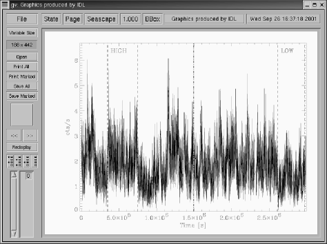
Figure 1: ASCA SIS0 light curve of Ark564. The dot–dashed thick line divides the light curves in two halves used to investigate stationarity. The dashed lines define two intervals used to characterize the timing behavior during the low and high count rate states.

In an attempt to answer this question and, more generally, to investigate the nature of the X-ray variability, we focus on a prominent object of a particular class of AGN, the Narrow-Line Seyfert 1 galaxies (NLS1), which often display rapid, large amplitude X-ray variability as well as extreme long-term changes (Forster & Halpern forst (1996), Boller et al. (1997), Brandt et al. (1999)), and therefore represent the ideal objects for an X-ray temporal analysis. In particular we analyze a recent long ASCA observation of Ark~564, the brightest NLS1 in the 2-10 keV band, using non-standard (at least for X-ray astronomy) analysis techniques.

The outline of this paper is the following. In Sect. 2 we describe the data used for the timing analysis. In Sect. 3 we investigate the important issue of the stationarity of a time series, by dividing the light curve into two equal parts and by computing and comparing the mean, the variance, the auto-correlation and structure functions and the power spectra of the two halves. Sect. 4 deals with the search for nonlinearity. To this end, we choose two parts of the light curve with reasonable length ($\sim$ 4 days), when the source was at a high and low count rate state, respectively. We use a new technique based on the constrained randomization of a time series and the nonlinear prediction error as an indicator of nonlinearity, in order to test the hypothesis that the light curve is a realization of a linear process. In Sect. 5 we first investigate the variability behavior of the source, utilizing both standard (excess variance, probability density function) and non–standard (fractals) techniques. Then, in order to investigate further whether the behavior of the source is identical in the two states (high and low) we used techniques like the phase space reconstruction and the scaling index method. Finally, in Sect. 6 we draw the main conclusions.

Figure 2: ASCA SIS0 light curves of Ark564 during the high (top panel) and the low (bottom panel) count rate state. Time bins are 16s. Both light curves contain 10000 data points each.

2 Data

Ark~564 was observed by ASCA from 2000 June 01 11:51:27 to 2000 July 05 23:57:54. We extracted the X-ray data from the public archive at ISAS and applied standard criteria for the data analysis in order to create light curves. Source counts were accumulated from a $\sim 8\arcmin\times 8\arcmin$ rectangle in detector coordinates to maximize the X-ray signal for the SIS0. The background was estimated from the source free region on the same chip and its level was less than 3% of the source count rate. During the analysis it became apparent that all instruments suffered from unexpected light leaks. This is probably due to an expansion of the atmosphere caused by recent solar activity and to the low satellite orbit during the observation. We investigated this light leak effect using energy spectra, low energy light curves, and DFE curves for each of the individual data sets (each FRF file). We found that in the data screening the BR_EARTH criterion for the SIS data had to be changed from $20^{\rm o}$ to $35^{\rm o}$ for the 0.55–10 keV data. The background-subtracted light curve is plotted in Fig. 1. The reason for the selection of two sub-intervals with high and low mean count rate is explained in Section 3. Fig. 2 shows a blow-up of the light curves during the high (top panel) and low count rate state (bottom panel). In the following, we restrict our analysis to the energy range 0.7–10 keV, completely free of the light leak problem, and use data only from the SIS0 detector, which is the most sensitive (and therefore has the highest count rate).

3 Stationarity Check

A time series, as any other scientific measurement, has to provide enough information to allow the determination of the quantity of interest unambiguously and it is useful only if reproducible, at least in principle. In other words, all statistical properties derived from the time series analysis should be invariant under a shift of the time origin. This is the definition of a completely stationary process.

However for most of the physical processes, in particular in astrophysics, this severe requirement is not applicable and two weaker conditions (which nevertheless describe roughly the same physical behavior) are applied. As first requirement, the time series should cover a stretch of time which is much longer than the characteristic time scale of the system. A second important requirement is that the properties of the system generating the signal must not change during the observation period. This can be checked in principle by measuring statistical properties, as the mean and the variance for the first and the second half of the data available and verifying that their variations are within their statistical fluctuations.

However, in case of AGN X-ray light curves, these requirements are usually not fulfilled for the following two reasons. First, X-ray observations of AGN have typically a duration ranging between a few hours to a few days (in the best cases). This time interval is usually sufficient to accumulate energy spectra with good signal-to-noise ratio, but not to reveal the characteristic time scale of an AGN. Second, the AGN power density spectrum is characterized by a “red noise” power law component $P(f)\propto f^{-\alpha}$ (with $\alpha\sim 1.5$; e.g. Lawrence & Papadakis 1993), indicating the presence of temporal correlations. Therefore, even if the parameters of the power density spectrum do not change, other parameters as the mean can change. However, as demonstrated by Press (1978) and, more recently for NLS1 galaxies, by Leighly (leig1 (1999)), the differences in excess variance between the first and the second half of the light curve can be entirely ascribed to the weak nonstationary inherent in the red noise.

Table 1: Statistical comparison between first and second half of the light curve

Property	First half	Second half
Mean	$1.893\pm 0.004$	$1.727\pm 0.003$
Variance	$0.600\pm 0.004$	$0.440\pm 0.003$
Skewness	$0.663\pm 0.013$	$0.625\pm 0.013$
Kurtosis	$0.732\pm 0.026$	$0.696\pm 0.025$

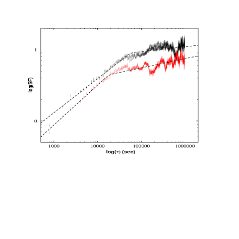
Figure 3: Structure function of Ark~564. The black error bars (upper curve) correspond to the first half of the light curve, the gray ones (lower curve) to the second half. The dotted lines show the best fitting “broken power law” model to the data.

Figure 4: Autocorrelation function of Ark~564. The filled circles correspond to the first half of the light curve, the open squares to the second half.

The long light curve of Ark~564 allows an accurate investigation of the stationarity of the source. For this reason, we divided the light curve into two equal parts, and computed not only the usual parameters, as the mean and the variance, but also the skewness and kurtosis (listed in Table 1) and estimated the structure and auto–correlation functions of the two halves.

The errors quoted in Table 1 were computed assuming that the data distribution is normal and the data are a collection of independent measurements. However, in the time series considered (and in general in all the AGN light curves) the measurements are not independent, but correlated. In this case, the actual errors, which might be much larger than the errors computed as explained above, cannot be easily quantified, since they depend on unknown quantities. For example, the actual error of the observed mean and variance depends on the true variance, on the true autocorrelation function of the underlying process and on the value of the power density spectrum at zero frequency (see Priestley 1989). Therefore, since the difference of the mean and variance between the two halves could be the result of the fact that red-noise processes are weakly non-stationary, we consider this difference as an indication, not as a proof, for stationarity.

To further investigate this issue we performed an analysis based on the structure function (e.g. Simonetti et al. (1985), Hughes et al. (1992)), which has the ability to discern the range of time scales that contribute to the variations in the data set. It is well known that structure functions are affected by the strong correlation between the points in the light curve. As with other statistics in the time domain, like auto and cross correlation functions, the points in the structure function are not independent, and the degree of their dependence is not easy to be determined in advance. However, the structure functions are not affected by the presence of missing parts in the light curves, therefore, their use can provide us with useful information in the case of unevenly sampled data, like in our case. For that reason, we computed the structure functions for the first and second half of the light curve. The results are plotted in Fig 3 (black and grey curve, respectively). The most important difference in Fig 3 is the time at which the structure functions reach a plateau state. By fitting a broken power law model to both structure functions, the best fit break time scale is $5.6^{+2.7}_{-1.8}\times 10^{4}{\leavevmode\nobreak\ \rm s}$ for the first part of the light curve and $1.8^{+1.2}_{-0.8}\times 10^{4}{\leavevmode\nobreak\ \rm s}$ during the second interval (the errors correspond to a 68% confidence level). This intrinsic difference in the temporal properties of the two halves of the light curve seems also to be reflected in the difference of the auto–correlation functions, estimated by using the Discrete Correlation Function (DCF) of Edelson & Krolik (1988). The rate at which the auto–correlation function decays to zero may be interpreted as a measure of the “memory” of the process and thus Fig 4 indicates that the “memory” of the second part of the light curve is shorter than that of the first part.

Like the mean and variance, the structure function and autocorrelation function of the first and second half of the light curve show differences. However, before reaching the conclusion that the light curve of Ark~564 is non–stationary, we should caution that it is very difficult to determine appropriate errors for the structure and autocorrelation functions and thus to assess the statistical significance of the apparent difference. (the reported errors basically give information about how many points contribute to each time scale.) We therefore tried to investigate further the stationarity using the power density spectrum (e.g. Papadakis & Lawrence pap2 (1995)) which, being the counterpart of the structure function in the Fourier domain, should provide the same information. In fact, detailed analysis of the power spectrum of the whole ASCA light curve of Ark 564 (Papadakis et al. 2002), together with the results of Pounds et al. (2001), shows that the power spectrum actually starts to flatten below $\sim 10^{-5}$ Hz, in agreement with the structure functions plotted in Fig 3. However, things are a bit more complicated when we divide the total light curve in two parts and compute their power spectra. The power spectrum is a much “noisier” function, when compared to the structure function. As a result, significant binning of the “raw” power spectrum is needed in order to investigate its shape. Without going into details of how the power spectrum was computed (see Papadakis et al. 2002), we simply mention that for a time series of 15 days length (corresponding to a minimum frequency of $7.7\times 10^{-7}$ Hz), after the necessary binning of the spectrum, the lowest accessible frequency is higher than $10^{-5}$ Hz. Therefore, all information about the possible presence of a break above $10^{5}$s is inaccessible and we cannot investigate if the location is different between the two parts of the light curve. Nevertheless, the overall power spectra of the two parts are consistent within the errors, a result that argues in favor of the the light curve being stationary.

Concluding, we can say that we find no strong evidence for non-stationarity. The mean, variance, structure function and autocorrelation functions of the two parts of the light curve do show differences, but these could be the result of the red-noise character of the observed variations. In fact, the power spectra of these parts show no statistically significant differences. However, since non-stationarity can affect the identification of genuine nonlinearity present in the data, and because of the presence of indications for non-stationarity (although not statistically significant) we decided not to utilize the whole data set for an investigation of the question of linearity of the light curve. Instead, we chose two parts that are “locally” stationary (meaning that after dividing them in two halves, no significant difference was found between the mean, variance, autocorrelation and structure functions of the first and second part), have reasonable length ($\sim 4$ days), and have different mean count rates. The selected “high” and “low” intervals, plotted in Fig 2, contain 10000 data points each (using a bin size of 16 s) with mean count rates of $2.14\pm 0.01{\rm\leavevmode\nobreak\ cts\leavevmode\nobreak\ s^{-1}}$ and $1.32\pm 0.01{\rm\leavevmode\nobreak\ cts\leavevmode\nobreak\ s^{-1}}$, respectively. In this way, apart from checking whether the light curve is nonlinear or not, we can also test if the source behaves differently in different flux states.

4 Search for nonlinearity

The search for nonlinearity in a time series is not only important but unavoidable in order to progress in the understanding of the origin of X-ray variability in AGN. In fact, various kinds of models (Gaussian, non-Gaussian, or nonlinear) have been proposed to explain the AGN variability. All of them are able to explain the red–noise power spectrum and other temporal characteristics such as the auto- and cross-correlation functions. However, it is important to stress that neither the power density spectrum nor the auto-/cross-correlation or structure functions are able to distinguish whether a process is linear or nonlinear (e.g. Vio et al. 1992).

Figure 5: Normalized real time series (top panel; mean = 0, $\sigma=1$) for the high state of Ark~564 and corresponding surrogate time series (bottom), which preserves the linear properties of the original data as mean, variance and auto–correlation function.

A relatively simple but sensitive method to test the presence of nonlinearity in a signal is the so called method of surrogate data (e.g. Theiler et al. 1992), which is based on the following ideas. First, one has to conceive a null hypothesis (for example, that the surrogates have the same linear properties as the real data) that we want to test against. Second, a level of significance for the test must be specified (a test valid at 95% significance level means that with a chance of $\alpha=0.05$ the null hypothesis is erroneously rejected). Then one creates a number of surrogate data according to the chosen null hypothesis ( $N_{\rm surr}=1/\alpha-1$ are created for a one–sided test, where the null hypothesis is rejected if the data deviate from the surrogates in a specified direction, whereas $N_{\rm surr}=2/\alpha-1$ are created in case of a two-sided test, where the data can deviate from the surrogates on either side). Finally one has to compare the real data with the surrogate time series using nonlinear statistics. If the real data differ significantly from the surrogates, nonlinearity can be inferred.

Standard surrogate methods (Theiler et al. 1992), make use of the Fourier transformation to conserve the auto–correlations of the original data: the original time series is rescaled to a Gaussian distribution first; then, the Fourier phases are randomized and the Fourier transformation is inverted. Finally, a rescaling to the original distribution is performed. However, such a method cannot be applied to unevenly sampled data (as the ASCA light curve of Ark~564), because it utilizes Fourier transformations and their inverses. Therefore, a more general approach based on the constrained randomization of a time series (Schreiber 1998) was used. In this new method, the desired properties (e.g. auto–correlations) of the surrogates are imposed by constraints: the surrogates start as a randomized distribution of the original data, and then are annealed until they match the ACF of the original data, at which point they are accepted as surrogates. The constraints are implemented as a cost function $E$ (e.g. Schmitz & Schreiber 1999), which is constructed to have a global minimum when the constraint is fulfilled (in simple words, if the constraint chosen is that surrogate data have the same auto–correlation as the real data, $E$ will be a function of the difference between the auto–correlations of real and surrogate data). Combinatorial minimization by complete enumeration is not feasible in case of long time series, since the computational effort grows exponentially with the length of the time series. Instead, we use the so called simulated annealing (e.g. Metropolis et al. 1953, Kirkpatrick et al. 1983), a powerful method for minimization in presence of many false (local) minima, that is expected to find an approximate solution in polynomial time.

Figure 6: Nonlinear prediction errors calculated from the surrogate data (shorter lines) and from the real data (longer thick dashed line) during the high state. The horizontal error bar indicates the standard deviation around the mean of the statistic computed from the surrogates.

The main idea behind the method of simulated annealing is to interpret the cost function $E$ as the energy in a thermodynamic system. Minimizing $E$ then is equivalent to finding the ground state of the system, and typically, for a glassy solid, this state is reached by first heating and subsequently cooling it (a procedure called “annealing”, hence the name of the method). In order to anneal the system to the “ground state”, that is, to the minimum cost function, we first “melt” the system at a high temperature $T$, and then decrease $T$ slowly. In practice, we started with a random permutation of the original time series and defined the starting cost function in the following way:

$$E=\left\{\sum_{i}\left[ACF_{\rm real}(i)-ACF_{\rm surr}(i)\right]^{2}\right\}^{1/2},$$ (1)

where $ACF_{\rm real}$ is the binned auto-correlation function of the real data and $ACF_{\rm surr}$ of surrogates. The surrogate is successively modified by exchanging randomly chosen pairs of elements and thus also the value of the cost function changes. The modification will be accepted with a probability $p=1$ if the energy decreases ($\Delta E<0$) and with $p=\exp(-\Delta E/T)$, where $T$ is a free parameter, if $\Delta E\geq 0$. Such updating scheme, proposed by Metropolis and collaborators (1953), allows the system to be close to the “thermodynamic equilibrium” at each stage. To summarize: the simulated annealing is performed by exchanging pairs of points (in the time domain) in each iteration step. Therefore, the surrogates have exactly the same distribution as the real data, i.e. they are “amplitude adjusted”. By keeping their autocorrelation function close to that of the original data all linear properties of the initial time series are preserved.

We repeated the whole procedure several times and created 39 independent surrogate data sets, necessary to perform a two–sided test for nonlinearity valid at 95% significance level or a one-sided test at 97.5% significance level (see below). Fig 5 shows the comparison between the real normalized time series (normalized to a mean$=0$ and $\sigma=1$) during the high state of Ark~564 and a corresponding surrogate time series (bottom), which preserves the linear properties of the original data like mean, variance and auto–correlation function.

After having produced randomized versions of unevenly sampled time series with given linear correlations, we use such surrogates to test for nonlinearity in the original data. In principle, any nonlinear statistic might be used, however, many statistics useful for evenly sampled time series cannot be easily generalized to unevenly spaced data. First we tried a simple but robust statistic which measures the time reversibility : $\gamma\propto\sum[y_{n}-y_{n-1}/(t_{n}-t_{n-1})]^{3}$, where $y_{n}$ denotes the count rate at time $t_{n}$ (e.g. Schmitz & Schreiber 1999). For a time series generated by a linear process, as in the case of surrogates, we expect $\gamma\simeq 0$. Since the measure of time reversibility of a time series generated by a nonlinear process can be either smaller or bigger than zero, we have performed a two–sided test. We found no statistically significant differences between real data and surrogates for both the low and high count rate states, i.e., the analysis does not support the hypothesis of a non-linear time series.

However, it must be pointed out that asymmetry under time reversal is a sufficient but not a necessary condition for nonlinearity. In addition, it has been demonstrated (Schreiber & Schmitz 1997) that, although the time reversibility is usually a good indicator of nonlinearity, in cases of very noisy data it can fail completely. According to Schreiber & Schmitz (1997), who systematically evaluated the abilities of different observables to detect nonlinearity, one of the best indicators is the nonlinear prediction error (e.g. Kantz & Schreiber 1997), which relies on the time delay embedding of a scalar time series, described in section 5.3.

The results of a one–sided test (the nonlinear prediction error for a nonlinear time series is expected to have lower values compared to the case of a linear time series) for the high count rate state are shown in Fig 6, where the value of the nonlinear prediction error for the original data is plotted with a longer thick dashed line, the mean and the standard deviation of the statistic obtained from the surrogates are represented by a cross and an error bar, respectively. It is evident that the original data are singled out by the estimate of the nonlinear prediction error and, therefore, the null hypothesis of a linear stationary process has to be rejected at 97.5% significance level. Applying the same procedure to the interval of the light curve corresponding to the low state of Ark~564, we reach a similar conclusion: nonlinearity is detected, although at a slightly lower (95%) significance level.

It must be noticed that also Edelson and collaborators (2002) searched for nonlinearity in this source and claimed a weakly significant (less than 1.5 $\sigma$) detection of nonlinearity. However, as the authors themselves remark, the method they used (the standard surrogate method) is not the best suited for the ASCA data of Ark~564.

Figure 7: Autocorrelation function of Ark~564 during the high (filled circles) and low (open squares) count rate states. Note that the range of the horizontal axis is a factor five smaller than that in Fig. 4.

Figure 8: Probability density function, normalized with respect to the average count rate $<cts>$ and standard deviation $\sigma$ for time series in the high (top) and low (bottom panel) count rate states.

5 Time Series Analysis of Ark~564

5.1 Standard Analysis

Detailed temporal and spectral variability analyses of the 35 day ASCA observation of Ark~564, based on power density spectra, cross–correlation functions are reported elsewhere (e.g. Turner et al. 2001, Edelson et al. 2002, Papadakis et al. 2002) and are beyond the scope of this work. Here, we investigate whether there are differences in the variability behavior of the source during the low and high state. We use standard techniques like the auto–correlation function and excess variance analysis, linear techniques that are not frequently applied to AGN light curves like the probability density function and, finally, fractal and nonlinear analysis techniques.

An analysis of the discrete auto–correlation functions (see Fig. 7), for the two chosen intervals seems to indicate that the high state (filled circles) is characterized by a slightly shorter characteristic time scale than the low count rate state (open squares), according to the narrower core of the former ACF. However, the most relevant quantity, the time lag at which the ACF decays to zero, is the same ($\tau\sim 2.5\times 10^{4}$ s) for both states.

To compare the degree of variability during the high and the low state (Fig. 2) we used the fractional variability amplitude $F_{\rm var}=\sqrt{(S^{2}-\langle\sigma^{2}_{\rm err}\rangle)/\langle X\rangle^{2}}$, where $S^{2}$ is the total variance, $\sigma^{2}_{\rm err}$ the mean error squared and $\langle X\rangle$ the mean count rate (e.g. Edelson et al. 2002). We found that during the low state the variability of the source was higher, $F_{\rm var}=(0.373\pm 0.003)$, than during the high state $(0.300\pm 0.002)$. It is worth noticing that from a recent temporal analysis based on $F_{\rm var}$ recently carried out on the ASCA light curve of Ark~564, Turner et al. (2001) found no clear correlation between the fractional variability and the X-ray flux.

We have compared the probability density functions for the time series of Ark~564 normalized with respect to the average count rate $<cts>$ and standard deviation $\sigma$ during the high and low state (see Fig 8). The two distributions look quite similar and differ from a Gaussian distribution (direct consequence of time correlations in the signal): both are characterized by a rather normal left-hand tail (related to the small amplitude events in the time series) and a right-hand tail following a power law trend. It is worth noticing that a qualitatively similar probability density function is displayed by two Galactic accreting objects, the micro-quasar GRS~1915+105 and the black hole candidate Cygnus X-1 and not by a non–accreting object as the Crab nebula (Greenhough et al. 2002).

5.2 Fractal Analysis

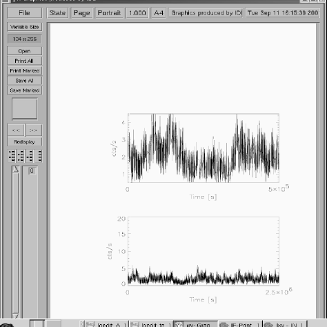
Figure 9: Interval of the light curve of Ark~564 shown with high resolution (top panel) and low resolution (bottom). Both axes are scaled by a factor of 5.

Fractals are now widely used in the modeling and interpretation of many different natural phenomena (see, e.g., Mandelbrot 1982, Pietronero & Tosatti 1986), including astrophysical phenomena (see, e.g., Heck & Perdang 1991). In this section, we use methods tailored for fractal analysis only as tools for extracting information from the signal, without considering the dynamical implications of the fractality. Our purpose is to go deeper into the comparison between the high and low count rate states, started in the previous section with standard techniques, by utilizing concepts characteristic of fractal analysis. In particular, after showing in a rather qualitative way that the light curve of Ark~564 can be considered as a fractal object (characterized by self-similarity and fractal dimension), we perform a quantitative comparison of their fractal properties based on the Hurst exponent (e.g. Kantz & Schreiber 1997)

AGN light curves, sampled with sufficiently high resolution, can be extremely complex and the scalar signal can be considered as a fractal, in the sense that its graph, as a function of time, has a nontrivial dimension. This means that the length of the graph seen at a finite resolution increases “forever” when the resolution on the time axis is increased, since more and more fluctuations are resolved. A priory there should not be a minimum time scale of variability in an AGN, apart from causality reasons. For example, a process which is the result of adding exponential shots will have a power density spectrum with a slope $-2$ extending towards infinite positive frequencies. Its dimension is, however, not an integer but lies anywhere between one and two, depending on the resolution. To visualize this concept let us consider a portion of the light curve of Ark~564 scaled in time and space by the same factor (see Fig 9). In the limit of high resolution (top panel), the graph tends to fill the plane and approaches dimension two, whereas in the opposite limit, it degenerates towards a horizontal line and thus to a dimension of one. Note that in this case the scaling factor is limited not by intrinsic physical reasons but by instrumental reasons (gaps due to earth occultation and low sensitivity). Moreover, approaching the resolution limit, the omnipresent noise component would hide the small-scale structures and the fluctuations would be washed out by measurement errors.

It must be noted that fractal properties, as the fractal length and dimension of the X-ray light curve of an AGN (the Seyfert 2 galaxy NGC~5506) were already investigated by McHardy and Czerny (1987), who derived some constraints on the emission mechanisms producing X-rays. Here, our main aim is not to repeat a similar kind of analysis, but to investigate the source’s behavior at low and high flux state, by comparing their fractal properties (i.e. their Hurst exponent, see below).

Figure 10: Flare of Ark~564 shown with increasing time resolution. The data points are connected with a line to show the averaged flare shapes.

In addition to a nontrivial dimension, fractals are characterized by self-similarity. A structure is said (strictly) self-similar if it can be broken into arbitrarily small pieces, each of which is a small replica of the entire structure. However, there are several variants of the mathematical definition of self–similarity. Dealing with erratic signals typical of AGN X-ray light curves, we are mainly interested in the “statistical self-similarity” and self–affinity, where the small “replica” may be somewhat distorted (for example skewed) with respect to the whole.

In the case of the light curve of Ark~564 this property can be evidenced by considering the same portion of the light curve with different resolution factors (i.e. with different time binning). In Fig 10 we focus on one of the many flares which occurred during the ASCA observation of Ark~564. It is shown that a rather smooth flare at low resolution (we started with a time binning equal to the orbital period) looks more and more complex when seen with increasing time resolution: each single flare observed at higher resolution is composed of several sub–flares. It can be seen that from 1408 s bins to 704 s bins the points start to cluster, indicating that the amount of variability on time scales shorter than 1000s is smaller. This is also reflected in the power density spectrum (Papadakis et al. 2002), which shows a break to a steeper slope around $\nu=10^{-3}$ Hz.

Figure 11: Logarithmic plot of the growth of range $\langle\Delta cts\rangle$. The filled circles refer to the high state while the diamonds to the low state.

The frequent gaps caused by earth occultation and the statistical fluctuations associated with measurement do not allow to use smaller time bins in the scaling down process. It is worth noting that also Tanihata et al. (tani (2001)) noticed a similar behavior in a recent study on time variability of blazars: none of the observed large flares show a smooth rise or decay but exhibit substructures, with smaller flares having shorter time scales.

Statistical self-similarity, although only for a limited time interval (as indicated by the breaks in the structure function and power density spectrum), seems to occur independently of the state of the source. In order to investigate quantitatively the scaling behavior of the light curve on short time scales (which are not accessible to visual inspection) during the high and low count rate states, we have calculated, for different time intervals $\Delta t$ (ranging from 32 to 1600 s), the difference between the maximum and the minimum count rates $\Delta cts$. Running this procedure over the portions of the light curve corresponding to the high and the low states for each $\Delta t$, an array of $\Delta cts$ is created from which the mean $\langle\Delta cts\rangle$ is found. For self–similar data $\langle\Delta cts\rangle\propto\Delta t^{H}$, where $H$ is called Hurst exponent (e.g. Kantz & Schreiber 1997) and ranges between 0 (for functions constant over time) and 1 (for functions increasing or decreasing linearly with time). Intermediate values of $H$ are generated by fractal functions, random Gaussian noise ($H\simeq 0.2$) and Gaussian random walk ($H\simeq 0.5$; typical for Brownian motion and normal diffusion process), whose increments possess a finite variance for every $\Delta t$ and are uncorrelated at successive time steps.

It is worth noticing that very different processes (e.g. hydrodynamical turbulence, standard and anomalous diffusion) are able to produce signals characterized by scaling laws and that they can be discriminated on the basis of their Hurst exponent. For example, this method has been used to quantify solar magnetic complexity (Adams et al. 1997), and the persistence of solar activity (Lepreti et al. 2000). Fig 11 shows the growth of range of $\langle\Delta cts\rangle$ for Ark~564 during the high (filled circles) and the low (open diamonds) state. The slopes, obtained from a linear least square fit, are very similar for the high ($0.29\pm 0.03$) and the low state ($0.28\pm 0.03$), indicating that the processes at work during the high and low state are of the same nature.

A similar analysis was performed by Greenhough and collaborators (2002) on very long RXTE light curves of three galactic objects: the Crab nebula, Cygnus X-1 and the micro-quasar GRS~1915+105. Interestingly enough, only the latter, which is thought to be a scaled down version of an AGN, had a Hurst exponent ($H\simeq 0.3$) consistent with the values found for Ark~564.

5.3 Nonlinear Analysis

Linear methods intrinsically assume that the dynamics of the system is governed by the linear paradigm: small causes lead to small effects. Since linear equations can only lead to exponentially growing (or decaying) solutions or to periodic oscillations, an irregular behavior of the system has to be attributed to some random external input. However nonlinear, chaotic systems can produce very irregular data with purely deterministic equations of motion. In other words, the apparently irregular and unpredictable behavior typical of X-ray light curves of AGN is not necessarily due to stochastic dynamics (i.e the action of a large number of excited degree of freedom). It might be also generated by chaotic dynamics of a limited number of collective modes: dissipation, coupling between different degrees of freedom and the action of an external field may lead to collective behavior (e.g. Eckmann & Ruelle 1985). The presence of nonlinearity in the X–ray light curve of Ark~564 leaves open the possibility that the light curve is produced by a chaotic system. However, it must be noted that nonlinearity is a necessary but not sufficient condition for a light curve to be produced by a chaotic system (Vio et al. 1992). In any case our main aim is not to discriminate chaos from stochasticity, but to compare the source’s behavior in the low and high state using nonlinear statistics. The scaling index method, the nonlinear statistics that we describe below, could be used even in the case of linear time series, since its ability to discern underlying structures in noisy data is not directly based on the nonlinear nature of the underlying process.

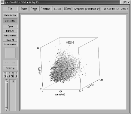
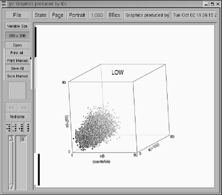
Figure 12: 3D–phase space portraits of the investigated portions of the light curve of Ark~564, with 10000 data points each. The time delay used to generate the artificial phase space is 100 times the temporal resolution of the time series. The units represent the number of photons contained in the smallest time bin (i.e. in 16s).

When methods of nonlinear dynamics are applied to time series analysis, the concept of phase space reconstruction represents the basis for most of the analysis tools. In fact, for studying chaotic deterministic systems it is important to establish a vector space (the phase space) such that specifying a point in this space specifies a state of the system, and vice versa. However, in order to apply the concept of phase space to a time series, which is a scalar sequence of measurements, one has to convert it into a set of state vectors. This is called phase space reconstruction and it is technically solved via the method of time delays and embedding. Starting from the original time series $X[t_{\rm i}]$ and introducing a time delay $\Delta t$, one can construct $d-1$ additional data sets $X[t_{\rm i}+\Delta t]$,…,$X[t_{\rm i}+(d-1)\Delta t]$, where $d$ is the dimension of the embedding space (the so called“embedding dimension”). The resulting $d$-dimensional artificial phase space represents all topological properties of the system in the real phase space, as long as the embedding dimension is twice the dimension of the real phase space (Takens 1981).

For illustration purposes we show in Fig 12 the three–dimensional pseudo phase space portraits of the light curve of Ark~564 during the high (top panel) and the low (bottom) state. Roughly speaking, the location of each point in the 3–D pseudo phase space (which is the simplest case, for a visual comparison between two data sets) is defined by three data points in the time series, which are separated by 100 and 200 steps, respectively ($X_{i+100}$ means an element displaced by 100 positions in the time series with respect $X_{i}$). The time delay is almost arbitrary. However, using too small time delays causes a clustering of the state vectors around the diagonal (due to the strong time correlations existing between successive elements of the vectors) and thus hamper the discrimination between the two data set under examination. On the other hand, the choice of a large delay value would reduce the number of points in the phase space, lowering the statistical significance of the analysis. Note that discontinuities in the time series due to earth occultation do not represent a problem for this kind of analysis, as far as the number of data points is sufficiently large for the reconstruction.

Figure 13: Spectrum of the scaling index distribution of Ark~564 during the high (solid line) and low (dashed line) states.

In order to quantify the difference between the phase space portraits in the high and low states, a suitable quantity is the correlation integral $C(r)$, which basically counts the number of pairs of points with distances smaller than $r$. This algorithm was introduced by Grassberger & Procaccia (1983) and was first used in astronomy to analyze light curves of variable stars (Auvergne & Baglin 1986) and binary systems (e.g. Voges et al. 1987), in order to put constraints on the origin of the irregular variability. An exhaustive description of the correlation integral method and its application to X–ray light curves of AGN is given by Lehto and collaborators (1993). An important property is that $C(r)$ at small r behaves as a power law and the exponent is closely related to the correlation dimension $D^{(2)}$ (Grassberger & Procaccia 1983), which for deterministic dynamical systems provides an estimate of the number of the degree of freedom excited, and more generally gives an indication of the “complexity” of the system.

The scaling index method (e.g. Atmanspacher et al. atma (1989)), which is based on the local estimate of the correlation integral for each point in the phase space, has been employed successfully in very different fields of the science for its ability to discern underlying structure in noisy data. A detailed description of this method and its application to astrophysics has been given by Williams et al. (willi (1998)). In practice, the scaling index method characterizes quantitatively the data point distribution by estimating the “crowding” of the data around each data point. For each of the N points, the cumulative number function is calculated

$$N_{i}(r)=\#\{j|d_{ij}\leq r\},$$ (2)

where $\#\{j\}$ indicates the number of points $j$, whose distance $d_{ij}$ from a point $i$ is smaller than $r$. The function $N_{i}(r)$ for each $i$ in a given range of radii (which are related to the typical distances between the data points, that, in turn, depend on the choice of the embedding space dimension) is approximated with a power law

$$N_{i}(r)\sim r^{\alpha_{i}}\,\,\,(r_{1}<r<r_{2}),$$ (3)

where $\alpha_{i}$ are the scaling indices. Explicitly, the $\alpha_{i}$ are given by

$${\alpha_{i}}=\frac{\log N_{i}(r_{1})-\log N_{i}(r_{2})}{(\log r_{1}-\log r_{2})},$$ (4)

Note that for a purely random process the average scaling index tends to the value of the embedding dimension, whereas for regular and for deterministic (chaotic) processes the value of $\langle\alpha\rangle$ is always smaller than the dimension of the embedding space.

It has been pointed out by Vio and collaborators (1992) that a naive application of the correlation integral method may lead to conceptual errors (as the detection of low–dimensional dynamics from signals produced by stochastic processes) and that this method must not be used in isolation, but as one of a collection of tests to discriminate chaos from stochasticity. Here we stress once more that the nonlinear statistics based on the scaling index is used only as a statistical test to discriminate between two states of the system, not to determine any kind of dimension, which would be meaningless for non-deterministic systems. The only requirement for the nonlinear discrimination of time series data, as for any statistical test, is that it must yield significant results.

We have calculated the scaling index for all the points of the two selected parts in the light curves using an embedding space of dimension 4 and suitable radii. There are no strong prescriptions for the choice of the embedding dimension. The discriminating power of the statistic based on the scaling index is enhanced using high embedding dimensions (this can be easily understood in the following way: if the data are embedded in a low-dimension phase-space many of them will fall on the same position, losing in this way part of the information). On the other hand, the choice of too high embedding dimensions would reduce the number of points in the pseudo phase-space, lowering the statistical significance of the test. We performed the scaling index analysis by increasing systematically the embedding dimension from 2 to 10, and found that a dimension of 4 is the best choice for the two investigated portions of the light curve with 10,000 data points each. The choice of the radii is also rather arbitrary, provided that Eq. (3) holds.

The resulting histograms are plotted in Fig 13. There is a remarkable difference between the two distributions, both in shape and location of the centroid. Such a difference cannot be ascribed to the fact that the data point distribution in the low state occupies a lower region in the pseudo phase-space with respect to the high space distribution. In fact the scaling index analysis is sensitive only to the relative positions of the data points within a distribution, not to their absolute positions in the phase space. For this kind of analysis the most important quantity is the location of the maximum of the histogram, which is related to the correlation dimension. Bearing in mind that the correlation dimension of a purely random data distribution tends to the value of the embedding dimension, the location of the maximum in the high state at a larger value indicates that the high state is “more random” or more “complex” (using a term borrowed from nonlinear dynamics) than that of the low count rate state. In other words, the high state is characterized by the action of a larger number of excited degrees of freedom.

6 Conclusions

We have carried out a thorough analysis of the timing properties of the NLS1 Ark~564, using the data from a recent long observation performed by the ASCA satellite.

The first important result is that we searched for signs of non–stationarity, without finding any strong evidence for it, although the differences in the structure function and autocorrelation functions between the first and the second part of the light curve give some indications in favor of a non–stationarity of the total light curve. To asses the stationarity of a time series is also important for a different aspect: the non-stationarity of the signal can strongly affect the identification of genuine nonlinearity possibly present in the data, and lead to wrong interpretations of results obtained from nonlinear statistical analyses.

As sensitive light curves long enough to cover several transitions between high and low states are presently not available, we concentrated on two sub–intervals of the Ark~564 light curve, which are locally stationary, contain a sufficiently large number of data points (10000, using a bin size of 16 s) for a meaningful statistical analysis, and which have significantly different mean count rates in order to characterize the intrinsic temporal differences from the low and the high state of the source.

We then carefully addressed the issue of the possible presence of nonlinearity, (often invoked as cause of giant flares in AGN light curves), which is crucial for breaking the degeneracy of models able to reproduce time-averaged spectra and some general timing properties. The result, obtained by utilizing a generalized surrogate method (well suited for unevenly sampled data) and the nonlinear prediction error, indicates the presence of nonlinearity both in the high and, at a slightly lower significance level, in the low count rate states. As a consequence, intrinsically linear models, where the variability is caused by many independent active regions, as magnetic flares or the traditional “shot noise” should be ruled out for Ark~564. Generalizations of these models, where the spatial and temporal distributions of flares are not random (e.g. Merloni & Fabian 2001) might still be a viable solution. The presence of nonlinearity favors nonlinear models as the self-organized criticality model or the emission from the base of a putative X-ray jet, as recently found in several radio-loud AGN. This last hypothesis seems to be supported also by two independent arguments: 1) the need of relativistic beaming effects to explain the extreme values for the efficiency in the conversion of gravitational potential energy into X-ray emission in several NLS1 galaxies (e.g. PKS~0558-504, Remillard et al.(1991); PHL~1092, Brandt et al. (1999); RX J1702.5+3247, Gliozzi et al.(2001)). 2) The recent discovery that, in a sample of 62 NLS1 detected in the FIRST VLA radio survey (Becker et al. (1995)), $\sim 40\%$ of the objects are radio–loud ($R>10$) and the remainder fall in the radio-intermediate range ($1<R<10$) (Whalen et al. 2002).

We then tried to characterize the timing behavior during the low and high count rate states of Ark~564. First, we used standard techniques (like the auto–correlation function and excess variance analysis) and linear techniques that are not frequently applied to AGN light curves (like the probability density function), without finding any significant difference between the two states. After showing that, for a limited time interval, the complex light curve of Ark~564 might be viewed as fractal objects with a non–trivial fractal dimension and statistical self–similarity, we tried to discriminate the two states with the help of the Hurst exponent. Also with this analysis no intrinsic differences were found, leading to the conclusion that the physical processes during the high and low state are of the same nature.

Finally, we have introduced the scaling index spectrum, based on phase space reconstruction, as a tool to discriminate time series. Based on this nonlinear statistic, we showed that the low and high states of Ark~564, apparently quite similar with respect to their linear properties, are intrinsically different, with the high state characterized by a higher degree of complexity, meaning that the number of degrees of freedom during the high state is larger that during the low state. However, in order to obtain firmer and more general conclusions we have to await further observations, in particular from the new X–ray missions, with sensitive, high time resolution instruments and the possibility of long continuous observations.