An analysis of gamma-ray burst spectral break models

Abstract

Typical gamma-ray burst spectra are characterized by a spectral break, $E_{p}$, which for bright BATSE bursts is found to be narrowly clustered around 300 keV. Recently identified X-ray flashes, which may account for a significant portion of the whole GRB population, seem to extend the $E_{p}$ distribution to a broader range below 40 keV. Positive correlations among $E_{p}$ and some other observed parameters have been noticed. On the other hand, within the cosmological fireball model, the issues concerning the dominant energy ingredient of the fireball as well as the location of the GRB emission site are still unsettled, leading to several variants of the fireball model. Here we analyze these models within a unified framework, and critically reexamine the $E_{p}$ predictions in the various model variants. Attention is focused on the predictions of the narrowness of the $E_{p}$ distribution in different models, and the correlations among $E_{p}$ and some other measurable observables. These model properties may be tested against the current and upcoming GRB data, through which the nature of the fireball as well as the mechanism and site of the GRB emission will be identified. In view of the current data, various models are appraised through a simple Monte-Carlo simulation, and a tentative discussion about the possible nature of X-ray flashes is presented.

1. Introduction

Gamma-ray burst (GRB) sub-MeV spectra contain most of the prompt information available from these mysterious sources. Progress in understanding the origin of such spectra, however, has been slow. A typical GRB spectrum is non-thermal, and can be fitted by a so-called Band-function (Band et al. 1993) with three parameters: a low energy power law photon index $\alpha$, a high energy power law photon index $\beta$, and the spectral break energy $E_{p}$ which defines the smooth transition between the two power laws. Since generally $\beta<-2$, $E_{p}$ is related to the peak of the $\nu F_{\nu}$ spectrum, and therefore is also called “E-peak”. Within the framework of the commonly considered cosmological fireball model, there are a number of variants (invoking different fireball contents, different emission sites, or different emission mechanisms) proposed to explain the GRB data. An important quantity which characterizes the GRB is $E_{p}$, which for 156 bright BATSE bursts in the 4B sample is found to be narrowly clustered around 300 keV, with a log-normal distribution with full width at half maximum of less than a decade (Preece et al. 1998; 2000). Theoretically, the value of $E_{p}$ is expected to be correlated with some other observational parameters, but such correlations could vary significantly in different models. These provide important criteria to evaluate the correctness of the models by comparing such correlations found in the data.

This topic has received heightened attention in view of two recent developments. On the one hand, a new category of X-ray transients, known as X-ray flashes (XRFs) has been identified (Heise et al. 2001; 2002, in preparation). The XRFs resemble normal GRBs in many respects, with the novelty that the peak energies are distributed from 100 keV to below 40 keV. These objects appear to form a natural extension of the GRB population in the softer and fainter regime (Kippen et al. 2001; 2002), which widens the narrow $E_{p}$ distribution found in the BATSE data, and it is estimated that XRFs represent a large portion (e.g. $\lower 4.0pt\hbox{$\buildrel<\over{\sim}$}1/3$) of the whole GRB population. It is therefore interesting to see how present theories can accommodate this new category of GRBs. On the other hand, GRB light-curve variabilities (Fenimore & Ramirez-Ruiz 2000; Reichart et al. 2001) and spectral lags (Norris et al. 2000; Norris 2002) have been proposed as Cepheid-like luminosity indicators for the long duration ($t_{b}\lower 4.0pt\hbox{$\buildrel>\over{\sim}$}2$ s) GRBs. These offer the exciting prospect of a direct relation between observable quantities and some of the theoretically most relevant parameters, such as the wind luminosity $L$, GRB intrinsic durations, emission-site magnetic fields, as well as the characteristic of the synchrotron or inverse Compton energies (which in many models are linked to the observed $E_{p}$). Empirically, some such correlations have been noticed. Lloyd-Ronning & Ramirez-Ruiz (2002) discovered a positive dependence of $E_{p}$ on the GRB variability (or luminosity). When combining this with the luminosity - variability correlation (Fenimore & Ramirez-Ruiz 2000; Reichart et al. 2001), one infers a positive correlation between $E_{p}$ and the burst luminosity $L$. Indeed, such a correlation has been seen in the BeppoSAX bursts with known redshifts (Amati et al. 2002). Thus, it is timely to critically revisit the physical $E_{p}$ predicted in various models, as a first step towards the goal of constraining or even identifying the nature of the fireball as well as the relevant emission site and mechanism for the GRB prompt emission. This is the purpose of the present paper. In §2.1, we present a synthesis of the current GRB model variants within a unified framework, and define the parameter regimes in which each model variant applies. In the rest of §2, we revisit these model variants, focusing specifically on the $E_{p}$ predictions. In §3, these predictions, as collected in Table 2, are used to evaluate the current models through a simple Monte-Carlo simulation, and the possible nature of the X-ray flashes is tentatively discussed. Conclusions are drawn in §4.

2. GRB models and $E_{p}$ predictions

2.1. GRB model synthesis

Cosmological fireball models invoke a brief release of energy $\sim 10^{51}-10^{53}~{}{\rm ergs}$ within a short duration of time $\sim 10^{-3}-10^{3}$ s. The fireball must be clean (low baryon load) so that after initial acceleration, the fireball is relativistic. The non-thermal spectrum requires the emission to be optically-thin, so that the emission site should be above the photosphere defined by the baryon content. The fireball eventually decelerates by the interstellar medium when the afterglow starts. The site of the GRB emission is therefore limited to the regime

$$r_{ph}\lower 4.0pt\hbox{$\buildrel<\over{\sim}$}r\leq r_{dec},$$ (1)

where $r_{ph}$ (e.g. eq.[3], see eq.[5] of Mészáros  et al. 2002 for a more general treatment) and $r_{dec}$ (eq.[2]) are the baryonic photosphere radius and the deceleration radius, respectively. The non-thermal nature of GRB emission also requires that the emission energy is not directly coming from the hot fireball (which gives a thermal-like spectrum), but derives from some other forms, e.g., the kinetic energy of the baryon bulk or the magnetic energy of the fireball. Generally, the GRB central engine involves a rapidly spinning and possibly highly magnetized object such as a black hole - torus system or a millisecond magnetar.

The fireball luminosity therefore may be broadly divided into two components. The first component, which is the component conventionally invoked in the simplest fireballs, is initially composed of thermal photons, pairs and a small amount of baryons. This component, which we call the hot component, essentially stores its energy in the form of the kinetic energy of the baryons after initial acceleration, apart from (usually) a small fraction of energy leaking at the baryonic photosphere. The second component, which we call the cold component, is carried by a Poynting-flux and low-frequency waves associated with the central engine spin. For ease of discussion below, we broadly define the hot and the cold luminosity components as $L_{h}\simeq L_{K}$ and $L_{c}\simeq L_{P}$, respectively, so that the total fireball luminosity is $L=L_{h}+L_{c}=L_{K}+L_{P}$. We also define the ratio of the cold-to-hot components as $\sigma\equiv L_{c}/L_{h}\simeq L_{P}/L_{K}$ following the convention of pulsar wind nebula theories (e.g. Rees & Gunn 1974; Kennel & Coroniti 1984). A fireball may be then defined as Poynting-flux-dominated if $\sigma\lower 4.0pt\hbox{$\buildrel>\over{\sim}$}1$ or as kinetic-energy-dominated if $\sigma\lower 4.0pt\hbox{$\buildrel<\over{\sim}$}1$. In principle $\sigma$ decreases with increasing radius due to conversion of part of the Poynting flux into the kinetic energy, especially when magnetic reconnection is operating, though the effect is likely not to be large (Lyubarsky & Kirk 2001; Contopoulos & Kazanas 2002). In any case, in the following discussions $\sigma$ refers to the specific value at the relevant radius in the problems.

The deceleration radius is defined by the kinetic energy of the fireball, $E_{K}=E/(1+\sigma)$, if the kinetic energy is decoupled from the magnetic energy by the time of deceleration, so that

$$r_{dec}=\left({3E_{K}}/{4\pi n_{ext}m_{p}c^{2}\Gamma^{2}}\right)^{1/3}$$

$$=5.4\times 10^{16}~{}{\rm cm}~{}E_{52}^{1/3}(1+\sigma)^{-1/3}n_{ext}^{-1/3}\Gamma_{2}^{-2/3},$$ (2)

where $n_{ext}$ is the density of the interstellar medium, $\Gamma$ is the bulk Lorentz factor of the fireball before deceleration, and hereafter the convention $Q_{n}=Q/10^{n}$ is adopted. The photosphere radius depends on a number of factors and has been discussed in Mészáros  et al. (2002) (see also §2.4). For a very clean fireball in which the opacity is defined by the thermal pairs rather than baryonic electrons,

$$r_{ph,\pm}=r_{0}(\Theta_{0}/\Theta^{\prime}_{\pm})=1.9\times 10^{9}~{}{\rm cm}~{}L_{52}^{1/4}(1+\sigma)^{-1/4}t_{v,m,-3}^{1/2},$$ (3)

where $\Theta^{\prime}_{\pm}\sim 0.03$ is the normalized (in unit $m_{e}c^{2}$) comoving temperature of the fireball when the pairs drop out of equilibrium (Shemi & Piran 1990; Paczyński 1986; Goodman 1986), and

$$\Theta_{0}=(k/m_{e}c^{2})(L_{h}/4\pi r_{0}^{2}\bar{\sigma})^{1/4}=1.9L_{52}^{1/4}(1+\sigma)^{-1/4}t_{v,m,-3}^{-1/2}$$ (4)

($\bar{\sigma}$ is the Stefan-Boltzmann constant, hereafter symbols like $m_{e}$, $m_{p}$, $c$, $e$, $\hbar$, etc. denote fundamental physical constants with conventional meanings) is the initial temperature of the fireball at the radius $r_{0}\sim ct_{v,m}=3\times 10^{7}~{}{\rm cm}~{}t_{v,m,-3}$ ($t_{v,m}$ is the minimum variability timescale of the central engine, which defines the width of each mini-shell to be $ct_{v,m}$), and $L_{h}=L/(1+\sigma)$ is the luminosity of the hot component. In the case where the baryon load is somewhat larger and the opacity is dominated by baryonic electrons, the photosphere radius is given instead by eq.(5) of Mészáros  et al. (2002). In any case, equation (3) marks the radius above which the pairs are no longer in equilibrium.

Another radius of interest is the critical radius where the MHD treatment breaks down, i.e., $r_{{}_{\rm MHD}}$. A convenient way to define $r_{{}_{\rm MHD}}$ is to require that the local plasma density, $n=n_{b}+n_{\pm}$ which includes both the baryon density and the pair density, to be equal to the Goldreich-Julian (1969, hereafter GJ) density, $n_{GJ}$, which is the minimum density required for the plasma to be frozen in the magnetic field (Usov 1994). The GJ density drops as $\propto r^{-3}$ within the light cylinder, $r_{lc}=c/\Omega$ (where $\Omega$ is the angular frequency of the central engine), but as $\propto r^{-1}$ beyond $r_{lc}$, so that at large distances, the GJ density is $n_{GJ}=(\Omega B_{s}/2\pi ec)(R/r_{lc})^{3}(r_{lc}/r)=(B_{s}R^{3}\Omega^{3}/2\pi ec^{3}r)$, where $R$ is the radius of the magnetized central engine. Assuming that the spin-down energy of the central engine is mainly carried by the Poynting flux, one has $L_{P}=B_{s}^{2}R^{6}\Omega^{4}/6c^{3}$. The GJ density in the rest frame of the fireball can be then expressed in terms of the measurable parameters (hereafter the primed quantities denote those measured in the rest frame of the fireball)

$$n^{\prime}_{GJ}=1.0\times 10^{8}~{}{\rm cm}^{-3}~{}[\sigma/(1+\sigma)]^{1/2}L_{52}^{1/2}t_{v,m,-3}^{-1}r_{13}^{-1}\Gamma_{2}^{-1},$$ (5)

where $t_{v,m}\sim 2\pi/\Omega\sim 10^{-3}$ s, and the value has been normalized to $r\sim 10^{13}$ cm which is the typical radius for the “internal” $\gamma$-ray emission (e.g. from the internal shocks). The comoving plasma density at the distance $r$ is $n^{\prime}=n^{\prime}_{b}+n^{\prime}_{\pm}$. For a continuous wind, the comoving baryon density $n^{\prime}_{b}=L_{K}/4\pi r^{2}m_{p}c^{3}\Gamma^{2}$ is

$$n^{\prime}_{b}=1.8\times 10^{13}~{}{\rm cm}^{-3}~{}L_{52}(1+\sigma)^{-1}r_{13}^{-2}\Gamma_{2}^{-2}.$$ (6)

The pair density is much lower than this. While they are in equilibrium, which is below $r_{ph,\pm}$ (eq.[3]) and generally somewhere below the baryonic photosphere, the pair number density is $n^{\prime}_{\pm}(th)\simeq 4.41\times 10^{30}{\rm cm}^{-3}{\Theta^{\prime}}^{3/2}\exp(-{\Theta^{\prime}}^{-1})$ (Paczński 1986). At the radius where $\Theta^{\prime}_{\pm}\sim 0.03$, this is $n^{\prime}_{\pm}(th)=7.6\times 10^{13}~{}{\rm cm}^{-3}$. Beyond the pair-freeze radius, $n^{\prime}_{\pm}$ drops as $\propto r^{-2}$, so that at the fiducial radius $r_{13}=1$, one has (cf. Usov 1994)

$$n^{\prime}_{\pm}\sim 2.8\times 10^{6}~{}{\rm cm}^{-3}~{}L_{52}^{1/2}(1+\sigma)^{-1/2}t_{v,m,-3}^{-1}r_{13}^{-2}.$$ (7)

In principle, further annihilation of these pairs is possible. In the context of the current problem, the annihilation time scale is much longer than the expansion timescale, so (7) generally applies. While $n^{\prime}_{\pm}<n^{\prime}_{GJ}$, the baryon density $n^{\prime}_{b}\gg n^{\prime}_{GJ}$ at small radii, although it will drop below $n^{\prime}_{GJ}$ at a large enough radius due to the different $r$-dependence of $n^{\prime}_{b}$ and $n^{\prime}_{GJ}$. By requiring $n^{\prime}_{b}\sim n^{\prime}_{GJ}$, one can define the radius where the MHD approximation breaks down, i.e.,

$$r_{{}_{\rm MHD}}=1.8\times 10^{18}~{}{\rm cm}~{}L_{52}^{1/2}[\sigma(1+\sigma)]^{-1/2}t_{v,m,-3}\Gamma_{2}^{-1}.$$ (8)

This radius is usually beyond the deceleration radius $r_{dec}$ (so that MHD approximation never breaks) unless

$$\sigma>\sigma_{c2}=190L_{52}^{3/4}E_{52}^{-1/2}t_{v,m,-3}^{3/2}n_{ext}^{1/2}\Gamma_{2}^{-1/2}$$ (9)

By setting $n^{\prime}_{b}=n^{\prime}_{\pm}$, one can also define a critical value

$$\sigma=\sigma_{c3}=4.1\times 10^{9}L_{52}t_{v,m,-3}^{2}\Gamma_{3}^{-4}~{},$$ (10)

above which the electrons associated with baryons are negligible.

Finally, there is another critical value of

$$\sigma=\sigma_{c1}\sim(0.1-1)~{},$$ (11)

which separates the regimes where strong shocks can or cannot develop. Strong shocks are only possible for low $\sigma$ flows. For $\sigma>\sigma_{c1}$, the shocks are quite weak, mainly because the three speeds on both sides of the shock are close to the speed of light (Kennel & Coroniti 1984).

A fireball may be classified into several sub-categories depending on the value of $\sigma$. Table 1 lists the characteristics of different fireball variants. GRB models can be also naturally classified into three categories based upon the proposed location of the GRB prompt emission. Within each category, several subtypes are defined according to the regime of $\sigma$, as follows.

1. Internal models, with $r_{ph}<r<r_{dec}$. In the standard scenario the energy input is an unsteady, kinetic-energy-dominated wind which undergoes dissipation in internal shocks (Rees & Mészáros  1994), which applies for $\sigma<\sigma_{c1}$. For $\sigma>\sigma_{c1}$, the source of energy dissipation may be from the strong magnetic fields in the fireball. For $\sigma>\sigma_{c2}$, the MHD approximation breaks down beyond the radius $r_{{}_{\rm MHD}}<r_{dec}$, and a global energy dissipation is expected to occur. For the extreme case of $\sigma>\sigma_{c3}$, the baryon content is negligible, and the process is analogous to a relativistic pulsar wind (Usov 1994; Lyutikov & Blackman 2001). For $\sigma_{c1}<\sigma<\sigma_{c2}$, the global MHD approximation applies all the way to the deceleration radius. Some local breakdown of the MHD condition is required (and possible), probably through magnetic reconnection (e.g. Drenkhahn & Spruit 2002).

2. External models, with $r=r_{dec}$. The standard picture is that of an external shock model (Rees & Mészáros 1992; Mészáros  & Rees 1993; Dermer, Chiang & Böttcher 1999). A variant of this model invokes the magnetic wind-medium interaction in the high-$\sigma$ regime (Smolsky & Usov 2000).

3. Innermost models, with $r\lower 4.0pt\hbox{$\buildrel>\over{\sim}$}r_{ph}$. Although the thermal nature of the photosphere emission seems to preclude its role as the main GRB emission mechanism, a few bursts are known to have quasi-thermal $\gamma$-ray spectra. A non-thermal character may also appear in the photospheric emission through Comptonization during the emergence of the spectrum (Goodman 1986). Also, with a strong magnetic component (not necessarily of very high $\sigma$), Alfvén turbulence induced and propagated from the deep layers beneath the baryonic photosphere can also lead to a non-thermal Compton tail (Thompson 1994; Mészáros  & Rees 2000). Even without Comptonization, both the baryonic and the pair photosphere components can provide additional components to the optically-thin component, and under certain circumstances even play a dominant role, which have been suggested to be responsible for the recently identified X-ray flashes (Mészáros  et al. 2002).

The most natural radiation mechanism in the optically thin region (both for the internal and the external models) is the synchrotron radiation (or its variants, e.g., jitter radiation, synchro-Compton radiation, random electric field radiation, etc.) and its self-inverse Compton (IC) emission, although the acceleration mechanism and the distribution function of the emitting electrons may vary in different models. For the baryonic photosphere Comptonization model, the $E_{p}$ is essentially defined by the thermal peak although the spectral shape is modified. Below we revisit the $E_{p}$ predictions in these model variants.

2.2. Internal models

Generally, the characteristic synchrotron emission energy (which is naturally connected to the $E_{p}$ energy in this model) of the electrons with typical energy $\gamma_{e}m_{e}c^{2}$ in a relativistic ejecta of bulk Lorentz factor $\Gamma$ is $E_{p}^{syn}=(4\Gamma/3)(3/2)\gamma_{e}^{2}(\hbar eB^{\prime}/m_{e}c)\sin\Psi(1+z)^{-1}$, or

$$E_{p}^{syn}\simeq 2\times 10^{-8}~{}{\rm eV}~{}(\Gamma B^{\prime})\gamma_{e}^{2}\sin\Psi(1+z)^{-1}.$$ (12)

where $B^{\prime}$ is the comoving magnetic fields, $\Psi$ is the mean pitch angle of the electrons, and $z$ is the source redshift. The factor $(\Gamma B^{\prime})$ is the Lorentz-boosted magnetic field strength, whose energy density should be proportional to the fireball energy density in the observer’s frame as long as the magnetic energy density is a constant fraction of the total energy density. This gives $\Gamma B^{\prime}\propto U^{1/2}\propto(L/r^{2})^{1/2}\propto L^{1/2}r^{-1}$, where $U$ and $L$ are the total energy density and the luminosity of the fireball. In principle there could be two components that contribute to the co-moving magnetic field in the emission region. The wind itself usually carries some “primordial” magnetic field ($B^{\prime}_{w}$) from the magnetized central engines, the lab-frame energy density of which can be estimated as $U_{B}=B_{w}^{2}/8\pi=L_{P}/4\pi cr^{2}$. The comoving field strength is then

$$B^{\prime}_{w}=[{2L\sigma}/{(1+\sigma)cr^{2}}]^{1/2}/\Gamma$$

$$\simeq 8.2\times 10^{5}~{}{\rm G}~{}[\sigma/(1+\sigma)]^{1/2}L_{52}^{1/2}r_{13}^{-1}\Gamma_{2}^{-1}.$$ (13)

Although such a large scale wind field is globally organized, we assume that in the dissipation regions (internal shocks or the reconnection sites) such a field is re-distributed randomly with comparable strength. Alternatively, magnetic fields could be generated in-situ ($B^{\prime}_{s}$) if the energy dissipation is through the internal shocks (e.g. Medvedev & Loeb 1999). Assuming that each proton gains a mean random energy $\theta_{p}m_{p}c^{2}$ from the internal shocks, the co-moving thermal energy density is $u^{\prime}=n^{\prime}\theta_{p}m_{p}c^{2}$, where $n^{\prime}$ is the comoving baryon number density in the shock-heated region. The parameter $\theta_{p}\sim(\gamma_{ij}-1)$ depends on the relative Lorentz factor between the shells, $\gamma_{ij}\simeq(\gamma_{i}/\gamma_{j}+\gamma_{j}/\gamma_{i})/2$, where $\gamma_{i}$ and $\gamma_{j}$ are the Lorentz factors of the two colliding shells, respectively. Though uncertain, $\theta_{p}$ is of order unity for typical parameters, and is not expected to be sensitive to the absolute value of $\Gamma$. When a collision occur, the slow shell enters the spreading phase due to the internal velocity difference within the shell itself. In this regime, the density in the shock-heated region evolves as $n^{\prime}\simeq\zeta M_{0}\Gamma/(4/3)\pi r^{3}m_{p}\sim\zeta Lt_{v}/(4/3)\pi r^{3}m_{p}c^{2}\propto r^{-3}$, where $M_{0}=Lt_{v}/\Gamma c^{2}$ is the total mass in the colliding shell, $t_{v}$ is the typical injection duration of the mini-shells, so that $\Delta_{0}\sim ct_{v}$ is the typical initial shell width, and $\zeta$ is the compressive ratio (at least 7 for strong shocks). If the shock-generated magnetic fields reach an equipartition fraction $\epsilon_{B}$ of the total thermal energy in the shock heated region, the co-moving field strength in the forward shocked region (in the slow shell) is then

$$B^{\prime}_{s}=(8\pi\epsilon_{B}n^{\prime}\theta_{p}m_{p}c^{2})^{1/2}$$

$$\simeq 1.4\times 10^{6}~{}{\rm G}~{}(\zeta_{1}\epsilon_{B,-1}\theta_{p})^{1/2}L_{52}^{1/2}r_{13}^{-1}\Gamma_{2}^{-1},$$ (14)

where $r\sim\Gamma^{2}\Delta_{0}$ (the internal shock radius) has been used. By comparing $B^{\prime}_{w}$ and $B^{\prime}_{s}$, we find that the wind component and the shock component of the magnetic fields have a similar amplitude for reasonable parameters, and share the same dependences on the parameters such as $L_{52}$, $r_{13}$ and $\Gamma$. This is understandable, since both the wind magnetic density and the shock magnetic density are assumed to be a constant fraction of the total energy density of the fireball (through $\sigma$ and $\epsilon_{B}$, respectively). For typical parameters, the co-moving field strength is $B^{\prime}=B^{\prime}_{w}+B^{\prime}_{s}=10^{6}~{}{\rm G}~{}\epsilon_{x1}L_{52}^{1/2}r_{13}^{-1}\Gamma_{2}^{-1}$, where $\epsilon_{x1}=0.82[\sigma/(1+\sigma)]^{1/2}+1.4(\zeta_{1}\epsilon_{B,-1}\theta_{p})^{1/2}$ for the internal shock models, or $\epsilon_{x1}=0.82[\sigma/(1+\sigma)]^{1/2}$ for the magnetic field dissipation models. We then have

$$\Gamma B^{\prime}=10^{8}~{}{\rm G}~{}\epsilon_{x1}L_{52}^{1/2}r_{13}^{-1},$$ (15)

which removes the apparent $\Gamma$-dependence (although $r_{13}$ is still dependent on $\Gamma$ in the internal shock models). Notice that even if $\epsilon_{B}\ll 1$ (as shown in the afterglow fits), $\epsilon_{x1}$ can be still close to unity given a large enough wind component (e.g. $\sigma>0.1$). Equation (15) is essentially model-independent.

The characteristic Lorentz factor of the emitting electrons $\gamma_{e}$, however, depends on the poorly understood mechanisms of particle acceleration. Conventionally, given a typical magnetic field at the acceleration site (eq.[15]), there are two characteristic $\gamma_{e}$’s from simple scalings. One is defined through the simple equipartition argument, i.e., to parameterize the random electron energy density to be proportional to the comoving thermal energy. Due to usually the same scaling laws of both densities, the typical electron Lorentz factor obtained using this method, denoted as $\gamma_{e}^{(1)}$, generally does not depend on the radius of emission and particle acceleration. A second estimate of $\gamma_{e}$, denoted as $\gamma_{e}^{(2)}$, is obtained by limiting the maximum gyro-acceleration at the local magnetic field by the synchrotron (and/or IC) cooling. For the simplest case, the typical acceleration time is $t^{\prime}_{a}=2\pi\gamma_{e}(m_{e}c/eB^{\prime})$, and the typical cooling time is $t^{\prime}_{c}=(\gamma_{e}m_{e}c^{2})/[(4/3)\gamma_{e}^{2}\sigma_{T}c({B^{\prime}}^{2}/8\pi)]$, where $\sigma_{T}$ is the Thomson cross section. Solving $t^{\prime}_{a}=t^{\prime}_{c}$, the maximum achievable electron Lorentz factor is

$$\gamma_{e}^{(2)}=(3/2)m_{e}c^{2}/[(2\pi)^{1/2}e^{3/2}B^{\prime 1/2}]=4.7\times 10^{4}{B^{\prime}}_{6}^{-1/2}.$$ (16)

This is radius-dependent (through different $B^{\prime}$ at different radii), but in such a form (e.g. $\gamma_{e}^{(2)}\propto{B^{\prime}}^{-1/2}$) that the comoving typical synchrotron frequency only depends on fundamental parameters. In the real problems, which of the two typical $\gamma_{e}$’s ($\gamma_{e}^{(1)}$ or $\gamma_{e}^{(2)}$) is relevant depends on the concrete conditions involved, and on the particle spectrum. Below we will discuss both the low $\sigma$ and high $\sigma$ cases for the internal models.

2.2.1 Low $\sigma$: internal shock dissipation

For the internal shock model, electrons are accelerated at the shocks via the Fermi mechanism to achieve a power-law distribution with the index $-p$. The minimum Lorentz factor of the injected electrons (i.e. $\gamma_{e}^{(1)}$ in the above notation) is $\gamma_{e}=f(p)({m_{p}}/{m_{e}})({\epsilon_{e}}/{\xi_{e}})\theta_{p}\simeq 310\epsilon_{x2}$, where $\epsilon_{e}$ is the electron equipartition factor which is believed to be close to unity (e.g. 0.3) in the internal shocks, $\xi_{e}$ is the injection fraction of the electrons which could in principle be less than unity (Bykov & Mészáros  1996; Daigne & Mochkovitch 1998), $f(p)=(p-2)/(p-1)$, and the typical value $1/6$ as $p=2.2$ has been adopted to get the numerical value. The parameter $\epsilon_{x2}=[{f(p)}/{(1/6)}]({\epsilon_{e}}/{\xi_{e}})\theta_{p}$ could be of order unity, if $\xi_{e}$ is below unity for more than an order of magnitude. One important feature of the internal shock model is that $\theta_{p}$, and therefore $\gamma_{e}$ only depends on the relative Lorentz factor between the colliding shells, which should not strongly depend on the actual bulk Lorentz factor of the shell, $\Gamma$, or the radius of the emission region, $r\propto\Gamma^{2}$. Notice that in this paradigm, $\gamma_{e}^{(2)}$ (eq.[16]) defines the maximum acceleration energy of the electrons, and is much larger than $\gamma_{e}^{(1)}$ ($\sim 310$), and $\gamma_{e}^{(1)}$ is relevant in the problem. Re-writing (12), we get the peak energy of the internal shock synchrotron model,

$$E_{p}^{i}(low~{}\sigma)\simeq 200~{}{\rm keV}~{}\epsilon_{x3}(L_{52}^{1/2}r_{13}^{-1})(1+z)^{-1},$$ (17)

where $\epsilon_{x3}=\epsilon_{x1}\epsilon_{x2}^{2}\sin\Psi$. It is worth emphasizing that the $r^{-1}$ dependence in (17) infers that $E_{p}\propto\Gamma^{-2}$ (see also Ramirez-Ruiz & Lloyd-Ronning 2002).

In some cases, e.g., long $t_{v}$ (large $r$) or large $\xi_{e}$ (so that $\epsilon_{x2}$ is much below unity), the synchrotron peak is below the BATSE window, and the synchrotron self-inverse Compton component may be responsible for the BATSE emission (Panaitescu & Mészáros  2000). The peak energy in this model is $E_{p}^{IC}=\gamma_{e}^{2}E_{p}^{syn}$, or

$$E_{p}^{i,IC}(low~{}\sigma)\simeq 200~{}{\rm keV}~{}\epsilon_{x4}(L_{52}^{1/2}r_{13}^{-1})(1+z)^{-1},$$ (18)

where $\epsilon_{x4}=\epsilon_{x1}(\epsilon_{x2}/0.06)^{4}\sin\Psi$. In both eqs.(17) and (18), all the parameters related to the shock physics are absorbed into two single parameters, $\epsilon_{x3}$, $\epsilon_{x4}$, and the dependence, $E_{p}\propto L_{52}^{1/2}r_{13}^{-1}(1+z)^{-1}$ is valid for both the the synchrotron and IC components. Several caveats ought to be made for the IC-dominated spectrum. First, $\epsilon_{B}/\epsilon_{e}\ll 1$ is generally required to achieve a prominent IC component (Zhang & Mészáros  2001 and references therein). In the internal shock regions, the effective $\epsilon_{B}$ can not be too low below unity given a not too small wind component $B^{\prime}_{w}$ (e.g. $\sigma>0.1$). Second, an IC-dominant fireball is inefficient in converting energy to radiation since multi-IC components at even higher energies consume much more energy so that one requires a very large energy reservoir to begin with (Derishev et al. 2001). Third, since $\epsilon_{x3}\propto\epsilon_{x2}^{2}$ while $\epsilon_{x4}\propto\epsilon_{x2}^{4}$, the IC mechanism tends to produce a wider $E_{p}$ distribution than the synchrotron mechanism (see §3 and Fig.1 for more discussions).

2.2.2 High $\sigma$: magnetic dissipation

If a wind has a high $\sigma>\sigma_{c1}\sim(0.1-1)$, strong internal shocks may not occur. Alternatively, intense energy dissipation may occur through magnetic reconnection and/or plasma instability. For $\sigma_{c1}<\sigma<\sigma_{c2}\sim 190$, MHD does not break globally, but local dissipation is possible through reconnection. If reconnection occurs below the photosphere, the dissipated energy is used to accelerate the fireball bulk. Only when $\sigma$ is above some value could the energy dissipation occur beyond the photosphere (Drenkhahn 2002). For $\sigma>\sigma_{c2}$, the MHD approximation breaks down globally before the deceleration radius, and a more violent, global energy dissipation is possible. The particle acceleration mechanism in both cases is hard to delineate. For the local dissipation case, the in-principle-achievable electron energy may be defined by the DC component of the electric field, i.e., $\gamma_{e,M,DC}m_{e}c^{2}=eE^{\prime}l^{\prime}$, where $l^{\prime}\sim\Gamma c/\Omega\sim 10^{9}\Gamma_{2}l_{7}$ is typical comoving scale of the stripped wind which may be regarded as the characteristic reconnection scale, $E^{\prime}=\alpha(v_{A}/c)B^{\prime}$ is the comoving DC electric field, where $v_{A}\sim c$ is the Alfvén speed, and $\alpha$ is a poorly constrained parameter (Syrovatskii, 1981; Craig & Litvinenko 2002). This gives $\gamma_{e,M,DC}\sim 6\times 10^{11}\alpha$ for typical values, which is extremely high unless $\alpha$ is very small. In reality, such a linear acceleration would be disrupted by any perturbation perpendicular to the DC direction, and the maximum achievable $\gamma_{e}$ may be still determined by the unavoidable perpendicular magnetic fields as well as the radiation self-reaction. Estimating the limiting $\gamma_{e}$ is difficult due to many uncertainties involved. In any case, if the electric and magnetic fields in the dissipation region could be regarded as quasi-random, the situation would be quite similar to the case of the global magnetic field dissipation, which we discuss below.

For $\sigma>\sigma_{c2}$, MHD breaks down at $r_{{}_{\rm MHD}}<r_{dec}$, and magnetic dissipation occurs globally. One possible consequence is that the MHD wind is converted to a large amplitude electromagnetic wave (LAEMW). The electrons may then surf and get accelerated in such a LAEMW (Gunn & Ostriker 1971; Michel 1984; Usov 1994; Chen, Tajima & Takahashi 2002). Alternatively and more plausibly, the LAEMW will soon evolves non-linearly and induces an electromagnetic turbulence through an overturn instability, so that the electromagnetic fields in the dissipation site are randomized (Lyutikov & Blackman 2001). Particles are stochastically accelerated and emit in the random fields. To estimate the maximum electron energy gained in the random field, we can use the two constraints that lead to the estimates $\gamma_{e}^{(1)}$ and $\gamma_{e}^{(2)}$, respectively. The first constraint is energy conservation. By assuming that a fraction $\epsilon_{e^{\prime}}$ of the co-moving local magnetic field energy density is eventually converted to the co-moving kinetic energy of the electrons, one can always write

$$\gamma_{e}m_{e}c^{2}\xi_{e}(n^{\prime}_{b}+n^{\prime}_{\pm})=\epsilon_{e^{\prime}}{B^{\prime}}^{2}/8\pi,$$ (19)

where $n^{\prime}_{b}$ and $n^{\prime}_{\pm}$ are the comoving baryon (and hence, baryon associated electron) and pair number densities, respectively. As discussed in §2.1, for the typical $\sigma$ of interest, $n^{\prime}_{b}\gg n^{\prime}_{\pm}$. Without generating additional pairs (which seem to be likely as discussed below), the emitting electrons are only those associated with the baryons, and this finally gives $\gamma_{e}^{(1)}\sim 2.8\times 10^{5}\epsilon_{x1}^{2}\epsilon_{e^{\prime}}\sigma_{2}\xi_{e}^{-1}$, which has no apparent $r$- or $\Gamma$-dependences since $n^{\prime}\propto{B^{\prime}}^{2}\propto(L^{\prime}/r^{2})$. Comparing to the typical $\sim 310$ in the internal shock models, this $\gamma_{e}$ is too large to reproduce the observed $E_{p}$ in the synchrotron model, unless $\epsilon_{e^{\prime}}\sim 10^{-3}\ll 1$.

The second constraint due to radiation self-reaction would be more relevant in this case, since the electrons are directly accelerated in the random electric magnetic fields. A similar estimate as (16) can be made. In a random electromagnetic field, the acceleration due to the electric field parallel to the moving direction ($E_{\parallel}$) is much smaller than that due to the electric field perpendicular to the moving direction ($E_{\perp}$) so that the whole field may be regarded as a random magnetic field with effective strength $\hat{B}^{\prime}\sim\sqrt{2}B^{\prime}$ (Landau & Lifshitz 1975; Lyutikov & Blackman 2001). Substituting $B^{\prime}$ by $\hat{B}^{\prime}$ in (16), the maximum achievable electron Lorentz factor is $\gamma_{e}^{(2)}\sim 3.9\times 10^{4}{B^{\prime}}_{6}^{-1/2}$. This gives the typical comoving synchrotron frequency ${E^{\prime}}_{syn}\sim 30~{}{\rm MeV}$. Obviously, this is too high to meet the observations.

There are two possibilities. First, it could be that the turbulence scale is much less than the radiative scale $ct^{\prime}_{c}/\Gamma$, so that the electrons never reach the maximum acceleration, but are limited by the turbulence scale itself. This effectively lowers the achievable $\gamma_{e}$ by a constant factor without modifying the dependence laws (Lyutikov & Blackman 2001). One may assume

$$\gamma_{e}=\epsilon_{c}\gamma_{e}^{(2)}=3.9\times 10^{2}\epsilon_{c,-2}{B^{\prime}}_{6}^{-1/2},$$ (20)

so that

$$E_{p}^{i}(high~{}\sigma)\simeq 300~{}{\rm keV}\epsilon_{x5}\Gamma_{2}(1+z)^{-1}.$$ (21)

where $\epsilon_{x5}=\epsilon_{c,-2}\sin\Psi$. The drawback of this possibility is that the process is still inefficient, since a low $\epsilon_{c}\sim 10^{-2}$ again implies a very low $\epsilon_{e^{\prime}}\sim 1\%$ given $n^{\prime}_{\pm}\ll n^{\prime}_{b}$. This is in contrast to the motivation of the magnetic dissipation model (e.g. Drenkhahn & Spruit 2002) which aims to overcome the low radiation efficiency encountered in the internal shock models. The main reason for the low efficiency in this case is that for a higher $\sigma$ wind, there are less baryon-associated electrons emitting given a same total wind luminosity.

The second (more plausible) possibility is that the primary electrons do get accelerated close to $\gamma_{e}^{(2)}$ and emit the $\sim 30$ MeV photons in the co-moving frame. These photons will interact with the low energy photons (comoving energy $\sim 10$ keV) to produce pairs if the radiation density is high enough. The new pairs are accelerated via the same mechanism, and a pair cascade develops, until eventually the pair density $n^{\prime}_{\pm}=\xi^{\prime}_{\pm}n^{\prime}_{b}\gg n^{\prime}_{b}$, which limits the achievable $\gamma_{e}$ to be below $\gamma_{e}^{(2)}$ through the energy budget constraint (19). Since there are more leptons emitting (most being pairs), a higher radiation efficiency is achievable. Though the cascade process is hard to describe analytically, one may estimate the minimum multiplicity by demanding the typical comoving emission energy to be below the pair threshold, i.e., $\gamma_{e}^{2}(\hbar eB^{\prime}/m_{e}c)\lower 4.0pt\hbox{$\buildrel<\over{\sim}$}0.5$ MeV. This gives $\gamma_{e}=(0.5/30)^{1/2}\gamma_{e}^{(2)}\sim 5.0\times 10^{3}{B^{\prime}}_{6}^{-1/2}$. Assuming a high radiation efficiency, i.e., $\epsilon_{e^{\prime}}\sim(1/3)$ in eq.(19), the required minimum pair multiplicity is $\xi^{\prime}_{\pm}=19\sigma_{2}\epsilon_{e^{\prime},1/3}L_{52}^{1/4}r_{13}^{-1/2}\Gamma_{2}^{-1/2}$. This still results in too high an $E_{p}$. In reality, more pairs would be further produced as long as there is a substantial hard energy spectrum extended above the typical synchrotron energy, which would degrade the expected $E_{p}$ further. Notice that as long as optically thin to the pairs, the dependence $\gamma_{e}\propto{B^{\prime}}^{-1/2}$ is still valid, mainly because both the comoving pair threshold itself ($\sim 0.511$ MeV) and the comoving characteristic synchrotron frequency ($\sim 30$ MeV for the first generation) are constant. The expression (21) is still valid, with $\epsilon_{x5}$ being defined differently. The attractive feature of such a model is that the final $E_{p}$ scatter is only due to the dispersion of the bulk Lorentz factor $\Gamma$ and a parameter $\epsilon_{x5}$. This is favorable for the observed narrow $E_{p}$ distribution for the bright BATSE bursts (see §3 and Fig.1 for more discussions).

In the magnetic dissipation model, there could be also a self-IC component. However, since the synchrotron component already has too high an energy for the GRB emission, invoking IC as the GRB mechanism has to introduce some ad hoc assumptions. Also all the criticisms to the IC internal shock models apply here as well. We therefore do not discuss such a possibility further.

2.2.3 Optically-thick pair photosphere

For both the shock dissipation and the magnetic dissipation scenarios discussed above, there could be the possibility that secondary pairs are so abundantly generated that they form an optical thick screen for the emergence of the photons (e.g. Guetta, Spada & Waxman 2001; Kobayashi, Ryde & MacFadyen 2002; Mészáros et al. 2002). Therefore the observed GRB emission, at least for some cases, has undergone Compton multi-scattering. The emergent GRB spectrum is then expected to be regulated by the existence of the pairs. The existence of the pairs may smear out or even destroy the “clean” correlations discussed above. Due to the non-linear nature of the problem, simple analytic $E_{p}$ dependences (i.e., the substitution of eqs.[17] and [21]) are hard to provide without numerical simulations. In any case, Mészáros  et al. (2002) have shown that pairs tend to be self-regulated at a moderate optical depth of $\tau^{\prime}_{\pm}\sim$ a few, and the co-moving typical frequency $E^{\prime}_{p}\propto T^{\prime}_{\pm}/{\tau^{\prime}}_{\pm}^{2}$. Since the comoving effective pair temperature is insensitive to the shock radius as long as copious pairs are produced, such a case is analogous to the high-$\sigma$ magnetic dissipation case, but due to quite different reasons. The dependence $E_{p}\propto\Gamma(1+z)^{-1}$ is more or less retained, with the possible weak dependence on $r$ through $T^{\prime}_{\pm}$. More detailed numerical work is underway to test such a simple treatment (Ramirez-Ruiz et al. 2002, in preparation).

The condition for forming such a pair photosphere is subject to further investigation. Pilla & Loeb (1998) numerically simulated the pair production process in the internal shocks with certain model parameters, and found that the pair processes mainly distort the high energy part of the spectrum, with the low-energy synchrotron peak almost unaltered. This hints that at least for some parameter regimes (which may be large), the optically-thin synchrotron model (both low-$\sigma$ and high-$\sigma$ cases as discussed in §2.2.1, and §2.2.2) applies. Another caveat is that a pair-regulated emission component tends to have smoother lightcurves, since short time scale variability will be smeared out through multi-Compton-scattering (see, e.g. Lazzati 2002). This hints that at least for those skipy lightcurves with short time variability, such an emission component is not important.

2.3. External models

The physical conditions at the deceleration radius, in certain circumstances, also allows emission with typical energy in the BATSE band, both for the low $\sigma$ and the high $\sigma$ cases. The main difference for both cases is the origin of the magnetic fields in the energy dissipation regions.

For a low-$\sigma$ flow (e.g. $\sigma<0.1$), the picture is the familiar external shock model (Mészáros & Rees 1993). The comoving magnetic field is generated in-situ through turbulent motions to some fraction of the equipartition value, $B^{\prime}=(32\pi\epsilon_{B}n_{ext}m_{p}c^{2}\Gamma^{2})^{1/2}\simeq 40~{}{\rm G}~{}\epsilon_{B}^{1/2}n_{ext}^{1/2}\Gamma_{2}$. The typical electron energy is $\gamma_{e}=[(p-2)/(p-1)](m_{p}/m_{e})(\epsilon_{e}/\xi_{e})\Gamma=3.1\times 10^{4}(\epsilon_{e}/\xi_{e})[f(p)/(1/6)]\Gamma_{2}$, where $\Gamma$ is the Lorentz factor of the forward shocked region. The $E_{p}$ prediction in this model is

$$E_{p}^{e}(low~{}\sigma)=75~{}{\rm keV}~{}\epsilon_{x6}n_{ext}^{1/2}\Gamma_{2}^{4}(1+z)^{-1},$$ (22)

where $\epsilon_{x6}=\epsilon_{B}^{1/2}(\epsilon_{e}/\xi_{e})^{2}[f(p)/(1/6)]^{2}\sin\Psi$. It is interesting to note that $\Gamma$ appears to the fourth-power, which can magnify any small dispersion in $\Gamma$ and tend to broaden the $E_{p}$ distribution (see §3 and Fig.1 for more discussions). Another emission component in the low-$\sigma$ external shock scenario is emission from the reverse shock propagating into the ejecta. Compared with forward shocked region, the reverse shocked region has the same comoving magnetic field strength and the bulk Lorentz factor, but the typical random Lorentz factor is $\gamma_{e}^{r}=[(p-2)/(p-1)](m_{p}/m_{e})(\epsilon_{e}/\xi_{e})\Gamma^{r}=3.1\times 10^{2}(\epsilon_{e}/\xi_{e})[f(p)/(1/6)]\Gamma^{r}$, where $\Gamma^{r}\simeq\Gamma_{0}/2\Gamma$ is the Lorentz factor of the reverse shock in the rest frame of the undecelerated ejecta with the bulk Lorentz of $\Gamma_{0}$ (see e.g. Mészáros  & Rees 1997a; Sari & Piran 1999). The typical synchrotron frequency is therefore degraded with respect to that in the forward shock by a factor of $\Gamma^{2}$, and lies in the optical band for typical parameters. However, the IC emission off these soft photon fields by the electrons both in the reverse shock and the forward shock regions can result in MeV photons which may (partially) account for the GRB prompt emission (see Wang, Dai & Lu 2001 for detailed discussions). In any case, these IC components have high powers of the random Lorentz factors (either $\propto\Gamma^{2}(\Gamma^{r})^{4}$ or $\propto\Gamma^{4}(\Gamma^{r})^{2})$, and will have a similar or even broader $E_{p}$ distribution as the standard external shock model (eq.[22]). Hereafter we do not explicitly discuss these possibilities.

For the high-$\sigma$ case, the external shock variant is given by the interaction between a relativistic plasma stream and a magnetic barrier. As simulated by Smolsky & Usov (2000), the outcome is dependent on the energy density ratio between the plasma and the field, $\alpha=8\pi n_{ext}m_{p}c^{2}(\Gamma-1)/B^{\prime 2}$. In such a case, the comoving magnetic field $B^{\prime}$ is dominated by the primordial wind component at the deceleration radius, i.e., $B^{\prime}\sim 180~{}{\rm G}~{}L_{P,52}^{1/2}E_{K,52}^{-1/3}\Gamma_{2}^{-1/3}n_{ext}^{1/3}$. The energy of electrons accelerated in the electric field generated at the front of the magnetic barrier is typically $\gamma_{e}\sim(m_{p}/m_{e})\Gamma=1.8\times 10^{5}\Gamma_{2}$. The typical synchrotron energy is too high, and Smolsky & Usov (2000) invoke the synchro-Compton radiation in a LAEMW as the GRB radiation mechanism. The latter is essentially a synchrotron mechanism except that the comoving $B^{\prime}$ is now replaced as the amplitude of the LAEMW, which is $B^{\prime}_{w}\simeq 0.1\epsilon_{w,-1}B^{\prime}$, and that the typical electron energy is $\gamma_{e}\sim 200\epsilon_{\gamma}\Gamma\sim 2\times 10^{4}\epsilon_{\gamma}\Gamma_{2}$. This gives the right $E_{p}$ energy

$$E_{p}^{e}(high~{}\sigma)\simeq 880~{}{\rm keV}~{}\epsilon_{x7}\Gamma_{2}^{8/3}L_{52}^{1/2}E_{52}^{-1/3}n_{ext}^{1/3}(1+z)^{-1},$$ (23)

where $\epsilon_{x7}=\epsilon_{w,-1}\epsilon_{\gamma}\sigma^{1/2}(1+\sigma)^{-1/6}$. The main difference between (23) and (22) is the origin of $B^{\prime}$. The wind $B^{\prime}$ is determined by the properties of the central engine, while the shock generated $B^{\prime}$ depends on $\Gamma$. Thus the power of $\Gamma$ in (23) is 4/3 lower than that in (22), leading to less dispersion in $E_{p}$ for the same $\Gamma$ scatter (see Fig.1).

In both cases, pair production is likely not to be crucial in regulating the $E_{p}$, due to a much smaller compactness parameter involved.

2.4. Innermost models

Regardless of the $\sigma$ value, a prompt signal is emitted as soon as the fireball becomes Thomson thin. The typical energy of such a baryonic photosphere emission is defined by the photosphere temperature, which depends on the dimensionless entropy of the fireball. Our treatment below follows Mészáros  et al. (2002), with the modification that we include a Poynting flux component. Since this cold component is not in the form of photons initially, it is left out in calculating the temperature of the baryonic photosphere.

The compactness parameter of the fireball can be expressed as a dimensionless parameter, $\ell_{p,o}=(L\sigma_{T}/4\pi m_{p}c^{3}r_{0})\simeq 1.2\times 10^{12}L_{52}r_{0,7}^{-1}$. For the purpose of the following discussion, $L$ should be substituted by the “hot” component, $L/(1+\sigma)$. The photosphere radius is defined by the Thomson-thin condition, i.e., $\sigma_{T}n^{\prime}l^{\prime}=1$, where $l^{\prime}$ is the comoving length of the continuous wind or the discrete shell. There are two critical values of the dimensionless entropy in the problem, both of which are related to $\ell_{p,o}$. The first value $\eta_{c1}=\ell_{p,o}^{1/5}=2.5\times 10^{2}[L_{52}(1+\sigma)^{-1}r_{0,7}^{-1}]^{1/5}$ is the critical entropy below which the opacity is defined by a continuous wind rather than a discrete shell. The second value $\eta_{c2}=\ell_{p,o}^{1/3}=1.0\times 10^{4}[L_{52}(1+\sigma)^{-1}r_{0,7}^{-1}]^{1/3}$ is the critical entropy above which the photosphere occurs in the acceleration regime. The observer-frame photosphere temperature satisfies $\Theta_{ph}/\Theta_{0}=(\eta^{8/3}\eta_{c1}^{-10/3},\eta/\eta_{c2},1)$ for $(\eta<\eta_{c1},\eta_{c1}<\eta<\eta_{c2},\eta>\eta_{c2})$, respectively (eq.[6] in Mészáros  et al. 2002, see detailed derivation given there). If the GRB emission is due to Comptonization of the photospheric emission by the Alfvén turbulence (Thompson 1994), the resultant $E_{p}$ should resemble the thermal peak predicted by $\Theta_{ph}$. Noticing (4), we get

$$E_{p}(ph)(1+z)=2.8\Theta_{ph}m_{e}c^{2}=$$

$$\cases{11~{}{\rm keV}~{}L_{52}^{-5/12}(1+\sigma)^{5/12}t_{v,m,-3}^{1/6}\Gamma_{2}^{8/3},~{}&~{}$\eta<\eta_{c1}$;\cr 370~{}{\rm keV}~{}L_{52}^{-1/12}(1+\sigma)^{1/12}t_{v,m,-3}^{-1/6}\Gamma_{3},~{}&~{}$\eta_{c1}<\eta<\eta_{c2}$;\cr 2.7~{}{\rm MeV}~{}L_{52}^{1/4}(1+\sigma)^{-1/4}t_{v,m,-3}^{-1/2},~{}&~{}$\eta>\eta_{c2}$.}$$ (24)

This is an extension of the discussion in Thompson (1994), who only discussed the highest $\eta$ case. The total photosphere luminosity scales with the temperature, i.e. $L_{ph}/L_{0}=\Theta_{ph}/\Theta_{0}$. Its relative importance with respect to the internal component depends on the regimes where $\eta$ lies. For the low-$\sigma$ case, the internal shock component dominates when $\eta$ is small, e.g. $\eta<\eta_{c1}$, but the photosphere component starts to be prominent when $\eta>\ell^{1/4}\sim 10^{3}(1+\sigma)^{-1/3}$.

3. Testing models against data

We consider the following $E_{p}$-related observational properties:

(i) For the 5500 spectra of 156 bright BATSE bursts analyzed in Preece et al. (2000), the typical $E_{p}$ is 300 keV, and the distribution is a narrow lognormal with full-width at half-maximum of less than a decade. Since each burst has many spectra in this dataset, the result implies that the $E_{p}$ dispersion for a particular burst is also very narrow.

(ii) A substantial population of X-ray flashes has been recently studied, with typical $E_{p}\lower 4.0pt\hbox{$\buildrel<\over{\sim}$}$ 40 keV (Heise et al. 2001; Kippen et al. 2001). If these events have the same origin as normal GRBs, they extend the $E_{p}$ distribution to a wider range, but the small sample collected so far indicates that the log-normal shape seem to be violated (Kippen et al. 2002).

(iii) Statistically, a positive correlation between $E_{p}$ and the isotropic luminosity $L$, $E_{p}\propto L^{\delta}$ with $\delta\sim 0.5$, has been noted recently (Amati et al. for the BeppoSAX bursts, and Lloyd-Ronning & Ramirez-Ruiz 2002 for the BATSE bursts).

These properties, along with other information such as temporal variability, spectral lags, etc. are relevant quantities to be accounted for in a theoretical model. Below we will test the model $E_{p}$ predictions with the above observational facts. The model predictions are collected in Table 2.

3.1. Narrowness of $E_{p}$ distribution

To compare the narrowness of the $E_{p}$ distributions among different models, we performed a simple Monte Carlo simulation. Since we are concerned about the narrowness of the distribution rather than the absolute value of $E_{p}$ in different models (and the uncertain free parameters make it possible for all the models to adjust the absolute $E_{p}$ values to match the 300 keV typical value), we have adopted arbitrary units for the parameters so that $\log E_{p}$ peaks around 0. We randomly generated 40000 bursts with distributions of the unknown parameters as follows: (1) burst luminosities span three orders of magnitude with a $N(L)dL\propto L^{-2}dL$ distribution (such a luminosity function is the natural consequence of the universal jet model, Zhang & Mészáros 2002, Rossi et al. 2002; and has received preliminary support from the data, Schaefer, Deng & Band 2001; Schmidt 2001); (2) burst Lorentz factors span 1.5 orders of magnitude and are correlated with the luminosity as $\Gamma\propto L^{1/2}$ with random deviations (a positive $\Gamma-L$ correlation is expected in both the conventional and the universal jet models, e.g. Kobayashi et al. 2002; Rossi et al. 2002; Zhang & Mészáros  2002, and here we adopt the (1/2) power as an example); (3) burst redshifts are randomly distributed in the $(0-15)$ range (a more detailed distribution function following the star formation history of the universe essentially does not influence the width of the final $E_{p}$ distribution, introducing only a minor distortion of the distribution shape); (4) $\log t_{v}$, $\log(T^{\prime}_{\pm}/{\tau^{\prime}_{\pm}}^{2})$, $\log\epsilon_{x5}$, $\log\epsilon_{x6}$, $\log\epsilon_{x7}$, are randomly distributed between (0,1); (5) $\log n_{ext}$ is randomly distributed between (0,2), and the total duration $\log T$ is randomly distributed between (0,3); (6) $\log\epsilon_{x1}$ and $\log\epsilon_{x2}$ follow a standard Gaussian distribution with random deviations. (This is because the product of at least three random variables has a log-normal distribution, Ioka & Nakamura 2002). For comparison, we also let $\epsilon_{x3}=\epsilon_{x1}\epsilon_{x2}^{2}$ be represented by a unit lognormal itself for another realization. The $E_{p}$ predictions within the different models are calculated according to Table 2. The fluxes of the bursts are calculated according to the standard $(\Omega_{m},\Omega_{\Lambda})=(0.3,0.7)$ cosmology. Given a certain flux threshold, the histograms of the $E_{p}$ distributions for different models are plotted for comparison.

Figure 1 shows the $E_{p}$ distributions of various models. To take into account the flux threshold effect, only the bursts whose fluxes are among the top-three flux decades are selected (2962 bursts from a total of 40000 bursts simulated). For ease of comparison, we have plotted all the histograms with the same scale (which spans 10 orders of magnitude). The models in the different subplots are: (a) the internal shock synchrotron model, with both $\epsilon_{x1}$ and $\epsilon_{x2}$ distributed as a lognormal; (b) the same internal shock synchrotron model, but with $\epsilon_{x3}$ itself assumed to be a standard lognormal. (This would imply that the dispersions among $\theta_{p}$, $\epsilon_{e}$, $\epsilon_{B}$, etc. are small due to some unknown conspiracy); (c) the internal shock synchrotron-self-IC model corresponding to the synchrotron model (a); (d) the internal magnetic dissipation model, which also applies to the pair-dominated internal models; (e) external shock model; (f) external magnetic model; (g) baryonic photosphere model in the coasting wind regime; (i) baryonic photosphere model in the coasting shell regime; (j) baryonic photosphere model in the acceleration regime.

From Fig.1 the following conclusions can be drawn. 1. Given the assumed parameter distributions, neither the internal nor the external models can reproduce the narrow $E_{p}$ distribution found in the sample of bright BATSE bursts (Preece et al. 2000). In our simulations, it is found that the narrowness of the $E_{p}$ distribution depends on the number of the independent parameters involved in the model, the narrowness of the assumed distribution of each parameter, as well as the power of these parameters. The more independent parameters, or the higher the power to which a certain parameter is involved in a model, the broader is the resulting $E_{p}$ distribution. 2. The IC models (Fig.1c) and the external models (Fig.1e and 1f) are even less favored, due to the much wider distributions caused by high powers of some parameters in their $E_{p}$ expressions (e.g. $\propto\epsilon_{x2}^{4}$ for the internal shock IC model, and $\propto\Gamma^{4}$ in the external shock model). 3. The usual internal shock synchrotron model (Fig.1a) also involves many parameters, and therefore results in a broad $E_{p}$ distribution among bursts. However, assuming that some of the parameters are not independent, one can reduce the number of free parameters to obtain a narrower distribution (Fig.1b). 4. Both the internal magnetic model and the pair-dominated model invoke the least independent parameters, and have narrow $E_{p}$ distributions. However the simulated distributions are still about one order of magnitude broader than the $E_{p}$ distribution observed in the bright BATSE bursts. 5. Two sub-classes of the innermost model, (h) and (i), have very narrow $E_{p}$ distribution (due to much smaller powers of the parameters involved, eq.[24]). These are comparable to that of the bright BATSE bursts. However, it is likely that these emission components contribute only partially, and under certain circumstances, to the GRB prompt emission

Several caveats about our simulations are pertinent. First, our primary goal here is not trying to match the Preece et al results closely. To make such close comparisons, other effects such as the detector energy band and the instrument response function ought to be taken into account, and a much larger parameter space would need to be explored for every model. It is also possible that the intrinsic $E_{p}$ distribution is broader than what is found by Preece et al. (2000), as indicated by the growing population of the XRF sources. Instead, we have adopted a uniform set of parameters for different models, which allows an unbiased evaluation among the models. In fact, it may be possible to reproduce Preece et al’s results by adjusting the distribution function and the dispersion of the input parameters within a certain model. For example, Böttcher & Dermer (2000) have shown that Preece et al’s narrow $E_{p}$ distribution is reproducible even in the $E_{p}\propto\Gamma^{4}$ external shock model, by taking into account the instrumental effects and the flux threshold effect, although they had to fix some input parameters (e.g. $n_{ext}$). Our Fig.1 nonetheless clearly reveals the “relative” abilities of different models to generate a narrow $E_{p}$ distribution. Second, in our simulations most of the parameters are regarded as independent of each other. However, there may exist some intrinsic correlations among some parameters, and the conspiracy among these parameters can reduce the $E_{p}$ scatter to achieve narrower distributions (we have shown this effect in Fig.1a and 1b). More detailed work is needed to explore these intrinsic correlations. Finally, it is possible that the flux threshold influences the scatter of the distribution. In Fig.2, we have explored such flux threshold effects for a particular model (the internal magnetic model, same conclusion also applies to other models). The three subplots indicate different flux thresholds: (a) $E_{p}$ distribution of all the 40000 bursts; (b) that of the 2962 bursts whose fluxes are among the top three orders of magnitude; (c) that of the 848 bursts whose fluxes are among the top two orders of magnitude. We see that the $E_{p}$ distribution indeed gets narrower when raising the flux threshold, but the effect is only mild. This might be because the intrinsic $E_{p}$ scatter due to many unknown parameters has a similar effect in a very wide flux decades.

3.2. Nature of X-ray flashes

Following the reports of the identification of the XRFs as a type of cosmological explosions resembling GRBs (Heise et al. 2001, 2002; Kippen et al. 2001; 2002), several speculations on the nature of these objects have been proposed. Whether they smoothly join the GRB distribution or constitute a related but separate class, the $E_{p}$ distributions associated with these objects would depend on the possible models, some of which we discuss below.

1. Dirty fireballs? Based on the external shock model, Dermer et al. (1999) discussed a type of then-undiscovered objects with lower bulk Lorentz factors than conventional GRBs, and suggested that such dirty fireballs would typically have lower $E_{p}$ (due to the $E_{p}\propto\Gamma^{4}$ dependence). It is then natural to attribute the XRFs to such dirty fireballs (Heise et al. 2001). However, we note that a dirty fireball does not necessarily produce a low $E_{p}$ burst. In the optically thin internal shock model, equation (15) shows that the apparent $\Gamma$ dependence cancels out, and equation (17) indicates that a dirty fireball has a closer-in internal shock radius, hence a higher $E_{p}$ due to a higher magnetic field (Fig.3a). In the high $\sigma$ case or the pair-dominated case, and in the external models, a positive dependence of $E_{p}$ on $\Gamma$ is retained, and a dirtier fireball tends to produce a lower $E_{p}$ (Fig.3).

2. High redshift bursts? An interesting possibility is that XRFs are GRBs at much higher redshifts (e.g. $z>6$), which may thus be related to the death of the first stars in the universe (Heise et al. 2001). However, some of the other collateral evidence for high-$z$ location, e.g., time dilation for both the total durations and the individual pulses, is lacking, which casts some doubts on such an interpretation (Lloyd-Ronning 2002). This problem is made less severe by the fact that also in normal GRBs, the presence of such time dilation is less noticeable than the intrinsic dispersion, and becomes noticeable only when analyzing very large samples (e.g. Norris et al. 2000).

3. Off-beam GRBs? There is now strong evidence that at least a fair fraction of GRBs are collimated. This raises the possibility of interpreting the XRF phenomenon as being due to viewing angle effects. In a version of such models where a sharp jet edge is assumed (Yamazaki, Ioka & Nakamura 2002), XRFs are those off-beam GRBs in which the observer misses the bright jet cone. Such a model requires the XRFs to be very nearby, $z\lower 4.0pt\hbox{$\buildrel<\over{\sim}$}0.2$. The redshift measurement of one X-ray rich GRB 011211 (a close relative of XRFs) at $z=2.14$ seems to suggest that at least some XRFs may not be interpreted in this scenario. In the universal jet beam model (Rossi et al. 2002; Zhang & Mészáros 2002), the off-beam population is greatly reduced, but bursts observed at large viewing angles tend to be “dirty”. The possible connection of such a configuration to XRFs (within the framework of the collapsar models) has been suggested by Woosley et al. (2002 and references therein).

4. Photosphere-dominated fireballs? Mészáros  et al. (2002) suggest that XRFs may be accounted for within the standard fireball internal shock model with moderate redshifts, due to a dominant contribution of either the baryonic or the shock pair photosphere. A similar proposal in the high-$\sigma$ case has also been suggested (Drenkhahn 2002).

The first two speculations invoke the dispersion of one particular parameter, while the total $E_{p}$ dispersion is the combined dispersions of many independent parameters. Whether the influence of one particular parameter is prominent depends on how many independent parameters are involved, and what is the power of that particular parameter in the $E_{p}$ expression. To show this effect, we plot in Fig.3 the predicted $E_{p}$ as a function of $\Gamma$ in four models: (a) internal shock model; (b) internal magnetic model; (c) external shock model; and (d) external magnetic model. We find that the $E_{p}$ broadening due to the $\Gamma$ scatter is more evident for the external models in which high powers of $\Gamma$ are invoked. Such an effect also depends on the bandwidth of the detector. Only when the bandwidth is larger than the intrinsic scatter at a same $\Gamma$ could the broadening due to $\Gamma$ scatter be noticeable. For the same reason, the redshift scatter only contributes weakly to the $E_{p}$ scatter, so that the high redshift interpretation of XRFs is not quite plausible. The photosphere interpretation in fact invokes possibly two (or even more) emission components with different $E_{p}$ distributions. A natural expectation of this model is that the $E_{p}$ distribution of the GRB/XRF combined population may have a non-lognormal or even bimodal distribution, which seems not incompatible with the current small sample (Kippen et al. 2002). To identify the nature of the XRFs, clearly more data are needed, including both redshift measurements and spectral fits.

3.3. $E_{p}-L$ correlation

The positive correlation $E_{p}\propto L^{\delta}$, (Amati et al. 2002; Lloyd-Ronning & Ramirez-Ruiz 2002) also poses interesting constraints on the models. It is seen in Table 2 that the different models give different predictions for the $E_{p}-L$ dependence. The complications arise from the $E_{p}$ dependence on the unknown $\Gamma$ expected in these various models, since there is no simple way to relate $\Gamma$ to the observables. In the above Monte Carlo simulations, we have adopted a positive $\Gamma\propto L^{k}$ ($k=1/2$ specifically) correlation, which is consistent with the expectation of the theoretical models (Kobayashi et al. 2002; Rossi et al. 2002; Zhang & Mészáros 2002; Salmonson & Galama 2002). If one takes $k$ as a free parameter, some constraints on $k$ may be imposed by the observed $\delta$. For example, the internal shock synchrotron model could not give a positive $E_{p}-L$ correlation if $k>1/4$. Ramirez-Ruiz & Lloyd-Ronning (2002) also noticed this, and argued that their observed relation (Lloyd-Ronning & Ramirez-Ruiz 2002) can be only accommodated within the IC-dominated model with an additional assumption of a $\gamma_{e}\propto\Gamma$ (the $\Gamma^{-2}$ dependence thereby canceling out). However, we note that the IC-dominant picture is less favored for other reasons as discussed above. Similar analyses could be made for the other models. For example, both external models seem to predict a too steep $E_{p}-L$ correlation, unless the $\Gamma-L$ relation is rather mild. The internal magnetic model or the pair dominated model are however compatible with the data for reasonable parameters.

4. Conclusions

The nature of the GRB prompt $\gamma$-ray emission, including the emission site and the energy contents of the fireball, are still poorly known after more than 30 years of efforts. We have analyzed the various fireball model variants within a unified picture, and have revisited the $E_{p}$ predictions of different models. These models are tested against the current GRB spectral data with a simple Monte Carlo simulation, with attention to the narrowness of the distribution and its dependence on some of the physical parameters. Our aim is to set up a general theoretical framework to allow unbiased tests of these models against the known data. Based on the analysis in this paper, we can evaluate the existing fireball models as follows.

1. The internal shock model is generally regarded as the most attractive candidate for the prompt $\gamma$-ray emission of classical GRBs. The highly variable, spiky GRB lightcurves are naturally reproduced in such a model, and many studies have shown that it is successful in reproducing many of the GRB properties (e.g. Kobayashi, Piran & Sari 1997; Daigne & Mochkovitch 1998; Panaitescu, Spada, Mészáros  1999; Spada, Panaitescu, Mészáros 2000; Ramirez-Ruiz & Fenimore 2000; Guetta et al. 2001). Our findings in this paper indicate two important caveats for the internal shock model. First, unless the dispersions in the shock parameters (e.g. $\epsilon_{e}$, $\epsilon_{B}$, $\theta_{p}$, $p$, etc) are very small or there exist some intrinsic correlations among the parameters, the internal shock model generates an $E_{p}$ distribution (Fig.1a) which, even in the optimistic case, is at least one order of magnitude broader than the straight (i.e. not otherwise corrected) distribution given by Preece et al. (2000). The calculated distribution may be still compatible with the data if XRFs are included in the observations, which intrinsically broaden the $E_{p}$ distribution. Second, the synchrotron internal shock model may not be able to reproduce the $E_{p}-L$ positive dependence unless the $\Gamma$ distribution is un-related or weakly related to $L$, or some further assumption is made (e.g. Ramirez-Ruiz & Lloyd-Ronning 2002).

2. The high-$\sigma$ internal model could inherit most of the merits of the internal shock model, with some additional advantages such as a smaller $E_{p}$ dispersion and the right $E_{p}-L$ correlation. The caveat in such models is that they have so far been less well-studied than the internal shock models, including the basic particle acceleration and emission processes. It is also unclear how to lower the typical $E_{p}$ energy to the sub-MeV band, and the physical context of how a high-$\sigma$ flow is launched in a collapsar is not well explored. More investigations in this direction are desirable (e.g. Blandford 2002).

3. In both the shock and magnetic dissipation internal models, both a narrow $E_{p}$ distribution and the right $E_{p}-L$ correlation are attainable if a pair photosphere is formed. However, it is unclear how common such a situation would be. The sharp lightcurve spikes may be also hard to reproduce.

4. The prompt $\gamma$-ray emission predicted in external models is expected in most cases, unless the external medium is very under-dense or previous internal dissipation of the bulk kinetic energy has been highly efficient. Whether the observed GRB prompt emission is attributable to this component is in question. Our simulations show that these models produce too broad an $E_{p}$ distribution compared with other models, and probably a too steep $E_{p}-L$ correlation. Other arguments against such scenarios include the need for additional assumptions (blobs) and the inefficiency involved in interpreting the variability (Sari & Piran 1997, but see Dermer & Mitman 1999). An important feature of these models is that $E_{p}$ are positively dependent on the ambient ISM density $n_{ext}$, which is in principle a measurable parameter. This provides a potential test for the model. More broadband afterglow fits are needed before a significant statistical evaluation can be made. Even if the external scenario does not account for the GRB prompt emission, studies of such a model are nevertheless meaningful since they can explore the important bridge between the prompt emission and the afterglow.

5. The emission component coming directly from the baryon photosphere is expected to partially contribute to the observed GRB prompt emission. The $E_{p}$ distributions for different regimes are narrow, and $E_{p}-L$ correlations are easily accommodated at least in the regime where the emission is the strongest (i.e., $\eta>\eta_{c2}$). The best guess is that such a component appears mixed in with other components, and becomes important under certain conditions.

6. All the IC models tend to generate broader $E_{p}$ distributions as compared with their synchrotron counterparts. They are also less favored due to other reasons.

Finally, our entire discussion in this paper is within the context of a naked central engine. A more realistic scenario invokes the fireball-progenitor envelope interaction, e.g. in collapsar models, which is receiving increased attention. These would lead to additional emission components, which are beyond the scope of the current paper.

Table 1Fireball variants

Condition	Fireball properties
$\sigma\lower 4.0pt\hbox{$\buildrel<\over{\sim}$}\sigma_{c1}$	kinetic energy dominated, strong shocks possible
$\sigma_{c1}<\sigma\leq\sigma_{c2}$	Poynting dominated, MHD does not break globally, but may break locally, no strong shocks
$\sigma_{c2}<\sigma\leq\sigma_{c3}$	completely Poynting dominated, MHD breaks globally, no strong shocks, baryon electrons non-negligible
$\sigma>\sigma_{c3}$	completely Poynting dominated, MHD breaks globally, no strong shocks, baryon electrons negligible

Table 2Model predictions for $E_{p}$

Models	Sub-categories	$E_{p}$	Comments
	low-$\sigma$: internal shocks	$\propto\epsilon_{x3}L^{1/2}\Gamma^{-2}t_{v}^{-1}(1+z)^{-1}$	$\gamma_{e}^{(1)}$ relevant
Internal models	high-$\sigma$: magnetic dissipation	$\propto\epsilon_{x5}\Gamma(1+z)^{-1}$	$\gamma_{e}^{(2)}$ relevant
	pair photosphere	$\propto\Gamma T^{\prime}_{\pm}/{\tau^{\prime}}_{\pm}^{2}(1+z)^{-1}$	Comptonized spectrum
External models	low-$\sigma$: external shocks	$\propto\epsilon_{x6}\Gamma^{4}n_{ext}^{1/2}(1+z)^{-1}$	$B$ generated in-situ
	high-$\sigma$: plasma-barrier interaction	$\propto\epsilon_{x7}\Gamma^{8/3}L^{1/2}E^{-1/3}n_{ext}^{1/3}(1+z)^{-1}$	$B$ carried from the wind
	$\eta<\eta_{c1}\sim 250(1+\sigma)^{-1/5}$	$\propto L^{-5/12}t_{v,m}^{1/6}\Gamma^{8/3}(1+z)^{-1}$	wind coasting regime
Innermost models	$\eta_{c1}<\eta<\eta_{c2}$	$\propto L^{-1/12}t_{v,m}^{-1/6}\Gamma(1+z)^{-1}$	shell coasting regime
	$\eta>\eta_{c2}\sim 10^{4}(1+\sigma)^{-1/3}$	$\propto L^{1/4}t_{v,m}^{-1/2}(1+z)^{-1}$	shell acceleration regime

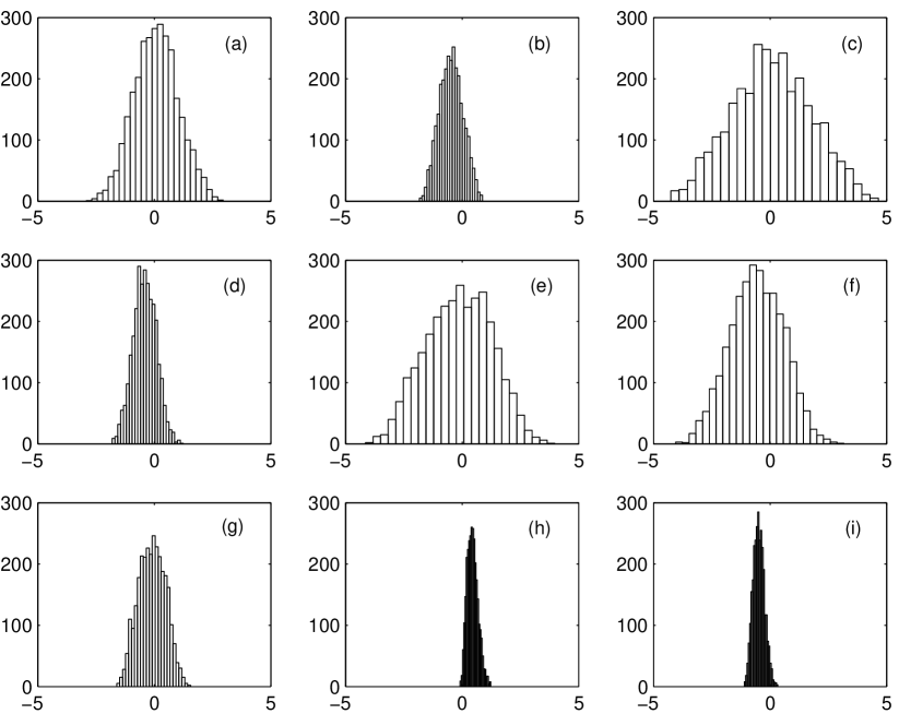
Figure 1.— $E_{p}$ distributions from Monte Carlo simulations for different models: (a) internal shock synchrotron model; (b) refined internal shock synchrotron model with a lognormal distribution of $\epsilon_{x3}$; (c) internal shock IC model; (d) internal magnetic dissipation model, or pair-dominated model; (e) external shock model; (f) external magnetic model; (g) baryonic photosphere model in the wind coasting regime; (h) baryonic photosphere model in the shell coasting regime; (i) baryonic photosphere model in the acceleration regime. The input parameters are described in the text. The histograms represent 2962 bursts whose fluxes are within the top three orders of magnitude, selected from a total 40000 bursts. Normalized $E_{p}$ values are used, with typical $\log E_{p}\sim 0$.

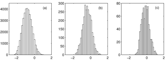
Figure 2.— The flux-threshold effect on the $E_{p}$ distribution in the simulations for Model (d) in Fig.1. (a) all 40000 bursts simulated; (b) the 2962 bursts whose fluxes are within the top three orders of magnitude; (c) the 848 bursts whose fluxes are within the top two orders of magnitude.

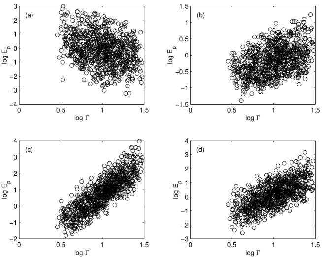
Figure 3.— Simulated $\log E_{p}$ as a function of $\log\Gamma$ in various models: (a) internal shock model; (b) internal magnetic model; (c) external shock model; (d) external magnetic model.

References

- (1) Amati, L. et al. 2002, A&A, 390, 81
- (2) Band, D. L., et al., 1993, ApJ, 413, 281
- (3) Blandford, R. D. 2002, in M. Gilfanov, R. Sunyaev et al. (eds), “Lighthouses of the Universe” Berlin: Springer, in press (astro-ph/0202265)
- (4) Böttcher, M., & Dermer, C. D., 2000, ApJ, 529, 635
- (5) Bykov, A. M., Mészáros, P. 1996, ApJ, 461, L37
- (6) Chen, P., Tajima, T. & Takahashi, Y. 2002, Phys. Rev. Lett., submitted (astro-ph/0205287)
- (7) Contopoulos, I., & Kazanas, D. 2002, ApJ, 566, 336
- (8) Craig, I. J. D., & Litvinenko, Y. E. 2002, ApJ, 570, 387
- (9) Daigne, F., & Mochkovitch, R. 1998, MNRAS, 296, 275
- (10) Derishev, E. V., Kocharovsky, V. V., & Kocharovsky, Vl. V. 2001, A&A, 372, 1071
- (11) Dermer, C. D., Chiang, J., & Böttcher, M. 1999, ApJ, 513, 656
- (12) Dermer, C. D., & Mitman, K. E. 1999, ApJ, 513, L5
- (13) Drenkhahn, G. 2002, A&A, 387, 714
- (14) Drenkhahn, G., & Spruit, H. C. 2002, A&A, submitted (astro-ph/0202387)
- (15) Fenimore, E. E., & Ramirez-Ruiz, E. 2000, ApJ, submitted (astro-ph/0004176)
- (16) Goldreich, P., & Julian, W. H. 1969, ApJ, 157, 869
- (17) Goodman, J. 1986, ApJ, 308, L47
- (18) Guetta, D., Spada, M., & Waxman, E. 2001, ApJ, 557, 399
- (19) Guibert, P. W., Fabian, A. C., & Rees, M. J. 1983, MNRAS, 205, 593
- (20) Gunn, J. E., & Ostriker, J. P. 1971, ApJ, 165, 523
- (21) Heise, J. in ’t Zant, J., Kippen, R. M. & Woods, P. M. 2001, in E. Costa, F. Frontera & J. Hjorth (eds) Gamma-Ray Bursts in the Afterglow Era, Proceedings of the International workshop held in Rome, CNR headquarters, 17-20 October, 2000, p16 (astro-ph/0111246)
- (22) Ioka, K., & Nakamura, T. 2002, ApJ, 570, L21
- (23) Kennel, C. F., & Coroniti, F. V. 1984, ApJ, 283, 694
- (24) Kippen, R. M., Woods, P. M., Heise, J., in ’t Zand, J., Preece, R. D. & Briggs, M. S. 2001, in E. Costa, F. Frontera & J. Hjorth (eds) Gamma-Ray Bursts in the Afterglow Era, Proceedings of the International workshop held in Rome, CNR headquarters, 17-20 October, 2000, p22 (astro-ph/0102277)
- (25) —–. 2002, to appear in proceedings of the Woods Hole GRB Workshop (astro-ph/0203114)
- (26) Kobayashi, S., Piran, T., & Sari, R. 1997, ApJ, 490, 92
- (27) Kobayashi, S., Ryde, F., & MacFadyen, A. 2002, ApJ, in press (astro-ph/0110080)
- (28) Landau, L. D., & Lifshitz, E. M. 1975, The classical theory of fields, Pergamon, Oxford
- (29) Lazzati, D. 2002, MNRAS, submitted (astro-ph/0206305)
- (30) Lee, H. K., Wijers, R. A.. M. J., & Brown, G. E. 2000, Phys. Pep., 325, 83
- (31) Lloyd-Ronning, N. M. 2002, in Woods Hole GRB conference proceedings (astro-ph/0202168)
- (32) Lloyd-Ronning, N. M., & Ramirez-Ruiz, E. 2002, ApJ, in press (astro-ph/0205127)
- (33) Lyubarsky, Y., & Kirk, J. G. 2001, ApJ, 547, 437
- (34) Lyutikov, M., & Blackman, E. G. 2001, MNRAS, 321, 177
- (35) Medvedev, M. V., & Loeb, A. 1999, ApJ, 526, 697
- (36) Mészáros, P., Ramirez-Ruiz, E., Rees, M. J., & Zhang, B. 2002, ApJ, submitted (astro-ph/0205144)
- (37) Mészáros, P., & Rees, M. J. 1993, ApJ, 405, 278
- (38) —–. 1997a, ApJ, 476, 232
- (39) —–. 1997b, ApJ, 482, L29
- (40) —–. 2000, ApJ, 530, 292
- (41) Michel, F. C. 1984, ApJ, 284, 384
- (42) Nakamura, T. 1999, ApJ, 522, L101
- (43) Norris, J. P. 2002, ApJ, submitted (astro-ph/0201503)
- (44) Norris, J. P., Marani, G., & Bonnell, J. 2000, ApJ, 534, 248
- (45) Paczyński, B. 1986, ApJ, 308, L43
- (46) Panaitescu, A., Spada, M., & Mészáros, P. 1999, ApJ, 522, L105
- (47) Panaitescu, A., & Mészáros, P. 2000, ApJ, 544, L17
- (48) Pilla, R. P., & Loeb, A. 1998, ApJ, 494, L167
- (49) Preece, R. D., et al. 1998, ApJ, 496, 849
- (50) —–. 2000, ApJS, 126, 19
- (51) Ramirez-Ruiz, E., & Fenimore, E. E. 2000, ApJ, 539, 712
- (52) Ramirez-Ruiz, E., & Lloyd-Ronning, N. M. 2002, New Astronomy, 7, 197
- (53) Reichart, D. E., et al. 2001, ApJ, 552, 57
- (54) Rees, M. J., & Gunn, J. E. 1974, MNRAS, 167, 1
- (55) Rees, M. J., & Mészáros, P. 1992, MNRAS, 258, P41
- (56) —–. 1994, ApJ, 430, L93
- (57) Rossi, E., Lazzati, D., & Rees, M. J. 2002, MNRAS, 332, 945
- (58) Salmonson, J. D., 2001, ApJ, 546, L29
- (59) Salmonson, J. D., & Galama, T. J. 2002, ApJ, 569, 682
- (60) Sari, R., & Piran, T. 1997, ApJ, 485, 270
- (61) —–. 1999, ApJ, 520, 641
- (62) Schaefer, B. E., Deng, M. & Band, D. L. 2001, ApJ, 563, L123
- (63) Schmidt, M. 2001, ApJ, 552, 36
- (64) Shemi, A., & Piran, T. 1990, ApJ, 365, L55
- (65) Spada, M., Panaitescu, A., & Mészáros, P. 2000, ApJ, 537, 824
- (66) Smolsky, M. V., & Usov, V. V. 2000, ApJ, 531, 764
- (67) Spruit, H. C., Daigne, F., & Drenkhahn, G. 2001, A&A, 369, 694
- (68) Syrovatskii, S. I. 1981, ARA&A, 19, 163
- (69) Thompson, C. 1994, MNRAS, 270, 480
- (70) Usov, V. V. 1992, Nature, 357, 472
- (71) —–. 1994, MNRAS, 267, 1035
- (72) van Putten, M. H. P. M. 2001, Phys. Rep., 345, 1
- (73) Wang, X. Y., Dai, Z. G. & Lu, T. 2001, ApJ, 556, 1010
- (74) Wheeler, J. C., Yi, I., Hoflitch, P. & Wang, L. 2000, ApJ, 537, 810
- (75) Woods, E., & Loeb, A. 1999, ApJ, 523, 187
- (76) Woosley, S. E., Zhang, W. & Heger, A. 2002, to appear in the Woods Hole GRB Workshop (astro-ph/0206004)
- (77) Yamazaki, R., Ioka, K., & Nakamura, T. 2002, ApJ, 571, L31
- (78) Zhang, B., & Mészáros, P. 2001, ApJ, 559, 110
- (79) —–. 2002, ApJ, 571, 876
- (80)