$1/f$ Noise and other Systematic Effects in the Planck-LFI Radiometers

We use an analytic approach to study the susceptibility of the Planck Low Frequency Instrument radiometers to various systematic effects. We examine the effects of fluctuations in amplifier gain, in amplifier noise temperature and in the reference load temperature. We also study the effect of imperfect gain modulation, non-ideal matching of radiometer parameters, imperfect isolation in the two legs of the radiometer and back-end $1/f$ noise. We find that with proper gain modulation $1/f$ gain fluctuations are suppressed, leaving fluctuations in amplifier noise temperature as the main source of $1/f$ noise. We estimate that with a gain modulation factor within $\pm 1\%$ of its ideal value the overall $1/f$ knee frequency will be relatively small ($<0.1$Hz).

1 Introduction

Planck is a European Space Agency (ESA) satellite mission to map spatial anisotropy and polarization in the Cosmic Microwave Background (CMB) over a wide range of frequencies with an unprecedented combination of sensitivity, angular resolution, and sky coverage (Bersanelli et al. bersanelli1 (1996)). Following the breakthrough of the COBE discovery of CMB anisotropy (Smoot et al. smoot (1992), Bennett et al. bennett (1996)), and the MAP satellite launched in June 2001, Planck will be the third generation space mission dedicated to CMB observations.

The data gathered by these missions will revolutionise modern cosmology by a precise determination of the fundamental cosmological parameters which govern the present expansion rate of the universe, the average density of the universe, the amount of dark matter, and the nature of the seed fluctuations from which all structures in the universe arose (see, e.g., Hu et al. Hu (1997), Scott et al. scott (1995), White et al. white (1994) for recent reviews on CMB anisotropy) and will provide at the same time full sky surveys at essentially unexplored frequencies, with fundamental implications for a large area of problems in astrophysics (De Zotti et al. dezotti (1999)).

Planck consists of a High Frequency Instrument (HFI) (Puget et al. puget (1998)) and a Low Frequency Instrument (LFI) (Mandolesi et al. mandolesi (1998)) observing the sky through a common telescope. While the MAP radiometers measure temperature differences between two widely separated regions of the sky through a pair of symmetric back-to-back telescopes, the Planck LFI radiometers are designed to measure differences between the sky signal and a stable internal cryogenic reference load. The LFI scheme takes advantage of the presence in the focal plane of the HFI front end unit, which is cooled to approximately 4 K as an intermediate cryo stage for the 0.1 K bolometer detectors.

The LFI radiometer design is a modified correlation receiver (Blum blum (1959), Colvin colvin (1961), Bersanelli et al. bersanelli2 (1995)), realised with High Electron Mobility Transistor (HEMT) amplifiers at 30, 44, 70 and 100 GHz. The modification is that the temperature of the reference load can be made significantly different from the sky temperature. To compensate for the offset (a few K in nominal conditions), a gain modulation factor, $r$, is used to null the output signal in order to minimise sensitivity to RF gain fluctuations and achieve the lowest white and $1/f$ noise in the output.

Obtaining data streams with low $1/f$ noise is of primary importance in order to achieve the LFI scientific objectives. In fact excessive $1/f$ noise would degrade the quality of the measured data (Janssen et al. janssen (1996)) by increasing the effective rms noise and the uncertainty in the power spectrum at low multipole values. Such effects can be avoided if the post detection knee frequency $f_{k}$ (i.e. the frequency at which the $1/f$ contribution and the ideal white noise contribution are equal) is significantly lower than the spacecraft rotation frequency ($f_{\rm spin}\sim 0.017$ Hz). For values of $f_{k}$ greater than $f_{\rm spin}$ it is possible to mitigate such effects by applying appropriate destriping and map making algorithms to the time ordered data (Maino et al. maino1 (2000)).

If the knee frequency is sufficiently low (i.e. $f_{k}\leq 0.1$ Hz), with the application of such algorithms it is possible to maintain the increase in rms noise within few % of the white noise, and the power increase at low multipole values (i.e. $l\leq 200$) at a very low level ($\sim$ two order of magnitude less than the CMB power). If, on the other hand, the knee frequency is high (i.e. $\gg 0.1$ Hz) then even after destriping the degradation of the final sensitivity is of several tenths of % and the excess power at low multipole values is significant (up to the same order of the CMB power for $f_{k}\sim 10$ Hz, Bersanelli et al., bersanelli2002 (2002)). Therefore, careful attention to instrument design, analysis, and test is essential in order to achieve a low $1/f$ noise knee frequency.

In this paper, we analyse the most important systematic effects due to non-ideal behaviour of components in the LFI radiometer signal chain, and estimate their impact on the post detection knee frequency. In section 2 we present a general analytical description of the Planck-LFI radiometers to derive formulas for the radiometer power output and sensitivity in the two cases of perfectly balanced and slightly unbalanced radiometer. Here we also show that under quite general assumptions, the radiometer sensitivity does not depend on the reference load temperature. In section 3 we analyse the impact of various systematic effects on the post-detection knee frequency showing that with proper gain modulation it is possible to keep the radiometer $1/f$ noise to a very low level also in the presence of different non-ideal behaviours (e.g., gain and noise temperature imbalance, imperfect gain modulation). For sake of conciseness, we transfer part of the formalism to the appendices. Finally, in section 4 we summarise our results and discuss briefly their implications for Planck observations.

2 Analytic model of LFI pseudo-correlation radiometers

2.1 Radiometer architecture

In Figure 1 we show a schematic of the baseline LFI radiometer design. In this design, each feed-horn is connected to a Radiometer Chain Assembly consisting of an actively-cooled 20 K front-end connected to a 300 K back-end via waveguides.

Figure 1: Schematic of the Planck LFI radiometer design. Each feed horn is connected to two radiometers constituted of a 20 K front-end and a warm back end at 300 K. In our design the reference load has a temperature of 4 K.

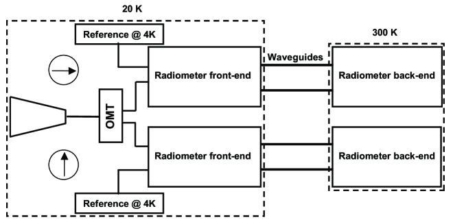
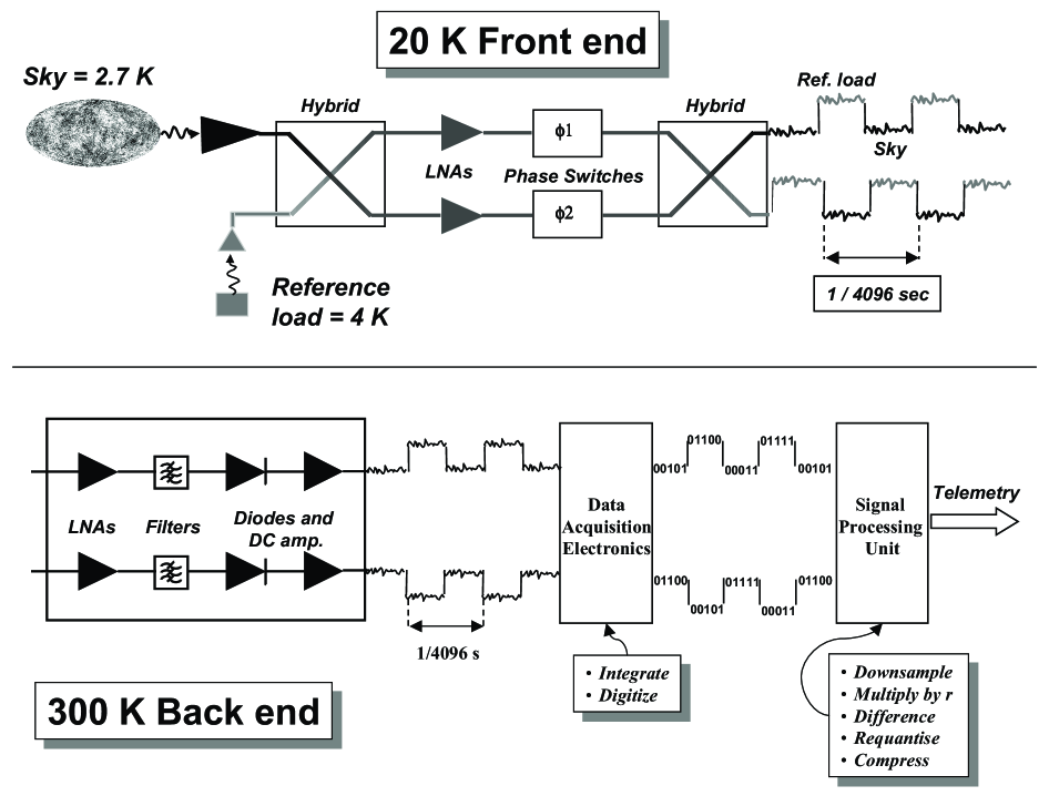
In the front-end part (see top part of Fig. 2) the radiation entering the feed-horn is separated by an OrthoMode Transducer (OMT) into two perpendicular linearly polarised components that propagate independently through two parallel radiometers. In each radiometer, the sky signal and the signal from a stable reference load at $\sim$4 K are coupled to cryogenic low-noise High Electron Mobility Transistor (HEMT) amplifiers via a $180^{\circ}$ hybrid. One of the two signals then runs through a switch that applies a phase shift which oscillates between 0 and $\pi$ at a frequency of 4096 Hz. A second phase switch will be present for symmetry on the second radiometer leg; this switch will not introduce any phase shift in the propagating signal. Therefore it will not be considered in our analysis. The signals are then recombined by a second 180^∘ hybrid coupler, producing an output which is a sequence of signals alternating at twice the phase switch frequency.

In the back-end of each radiometer (see bottom part of Fig. 2) the RF signals are further amplified, filtered by a low-pass filter and then detected. After detection the sky and reference load signals are integrated, digitised and then differenced after multiplication of the reference load signal by a so-called gain modulation factor, $r$, which has the function to make the sky-load difference as close as possible to zero.

Figure 2: Details of the front-end (upper figure) and back-end (lower figure) of LFI radiometers.

According to this architecture each radiometer will produce two independent streams of sky-load differences; the final measurement is provided by a further averaging of these differenced data samples between the two radiometer legs.

The LFI pseudo-correlation design offers two main advantages: the first is that the radiometer sensitivity does not depend (to first order) on the level of the reference signal; the second is provided by the fast switching that reduces the impact of $1/f$ fluctuations of back-end amplifiers. In the next subsection we present the analytical description of this radiometer design. In particular we derive formulas for the power output and sensitivity in the two approximations of (i) perfectly balanced and (ii) slightly unbalanced radiometer. Then we show how the radiometer sensitivity is not dependent, to first order, on the reference load temperature and we also provide an estimate of this dependence in the case of slightly unbalanced radiometer.

In order to improve readability we have kept the mathematical treatment as simple as possible, relegating the full definition of long formulas to appendices.

2.2 Analytic model of LFI radiometers

2.2.1 Input-output signal sequence

Referring to the schematic in Fig. 2, we can define the following transfer functions for the different radiometer components.

$$f_{\rm hyb}:\{x,y\}\rightarrow\left\{\frac{x+y}{\sqrt{2}},\frac{x-y}{\sqrt{2}}\right\}$$

$$f_{\rm amp}^{\rm FE}:\{x,y\}\rightarrow$$

$$\,\,\,\,\,\,\,\,\,\,\,\,\,\,\,\,\,\,\,\,\,\,\,\,\,\,\,\,\,\,\,\,\,\,\,\,\left\{g_{F_{1}}(x+n_{F_{1}})e^{i\phi_{F_{1}}},g_{F_{2}}(y+n_{F_{2}})e^{i\phi_{F_{2}}}\right\}$$

$$f_{\rm sw}:\{x,y\}\rightarrow\left\{x,\sqrt{A_{j}}e^{i\theta_{j}}y\right\}\,\,\,\,\,{\mbox{w}ith}\,j=1,2$$ (1)

$$f_{\rm amp}^{\rm BE}:\{x,y\}\rightarrow$$

$$\,\,\,\,\,\,\,\,\,\,\,\,\,\,\,\,\,\,\,\,\,\,\,\,\,\,\,\,\,\,\,\,\,\,\,\,\left\{g_{B_{1}}(x+n_{B_{1}})e^{i\phi_{B_{1}}},g_{B_{2}}(y+n_{B_{2}})e^{i\phi_{B_{2}}}\right\}$$

where:

• $x(t)$ and $y(t)$ represent the voltages at the sky and reference horns respectively;

• $g_{F_{1}}$, $g_{F_{2}}$, $g_{B_{1}}$ and $g_{B_{2}}$ are the voltage gains of front-end and back-end amplifiers;

• $n_{F_{1}}(t)$, $n_{F_{2}}(t)$, $n_{B_{1}}(t)$ and $n_{B_{2}}(t)$ represent the noise voltages of the front-end and back-end amplifiers;

• $\phi_{F_{1}}$, $\phi_{F_{2}}$, $\phi_{B_{1}}$ and $\phi_{B_{2}}$ represent the signal phases after the amplifiers;

• $\theta_{1}$ and $\theta_{2}$ represent the phase shifts in the two switch states (in LFI baseline $\theta_{1}=0$ and $\theta_{2}=\pi$);

• $A_{1}$ and $A_{2}$ represent the fraction of the signal amplitudes that is transmitted after the phase switch in the two switch states. For lossless switches $A_{1,2}=1$.

The output signal at the two radiometer legs is given by:

$$s_{j,1} = e^{i\phi_{B_{1}}}g_{B_{1}}\left\{n_{B_{1}}+\frac{1}{\sqrt{2}}\left[e^{i\phi_{F_{1}}}g_{F_{1}}\left(n_{F_{1}}+\frac{x+y}{\sqrt{2}}\right)+\right.\right.$$

$$+ \left.\left.\sqrt{A_{j}}e^{i(\theta_{j}+\phi_{F_{2}})}g_{F_{2}}\left(n_{F_{2}}+\frac{x-y}{\sqrt{2}}\right)\right]\right\}$$

$$s_{j,2} = e^{i\phi_{B_{2}}}g_{B_{2}}\left\{n_{B_{2}}+\frac{1}{\sqrt{2}}\left[e^{i\phi_{F_{1}}}g_{F_{1}}\left(n_{F_{1}}+\frac{x+y}{\sqrt{2}}\right)+\right.\right.$$

$$- \left.\left.\sqrt{A_{j}}e^{i(\theta_{j}+\phi_{F_{2}})}g_{F_{2}}\left(n_{F_{2}}+\frac{x-y}{\sqrt{2}}\right)\right]\right\}$$

where the subscript $j=1,2$ indicates the two phase switch states.

2.2.2 Radiometer power output and sensitivity

Our first step is to write an expression for the radiometer power output at a given time $t$, considering that in our scheme we take the difference between the sky and load signals. If we indicate with $p_{\,l}(t)$ the power output at each of the two radiometer legs (where $l=1,2$) and with $p\,(t)$ the radiometer power output we have that:

$$p_{\,1}(t)=a\left(|s_{1,1}|^{2}(t)-r|s_{2,1}|^{2}(t+\Delta t_{\rm sw})\right)$$

$$p_{\,2}(t)=a\left(|s_{2,2}|^{2}(t+\Delta t_{\rm sw})-r|s_{1,2}|^{2}(t)\right)$$ (3)

$$p\,(t)=1/2\left[p_{1}(t)+p_{2}(t)\right]$$

where $a$ is the constant of proportionality of the square-law detectors, $\Delta t_{\rm sw}\sim 122$ $\mu$s corresponds to half of the phase switch period and $r$ is the gain modulation factor which in LFI scheme is applied in software. The expanded form of $p_{\,1}(t)$ is reported in equation (28); a similar relationship holds for $p_{2}(t)$. The assumption of identical values of $a$ in the above equation can be made without loss of generality; any difference in actual values between the two legs could be absorbed into back-end gain differences for the purposes of this analysis.

In our treatment we will show how the gain modulation factor (a real number generally $\leq 1$) can be tuned properly in order to have an approximately null power output, which leads to almost complete suppression of the dependency of the radiometer sensitivity on the reference load signal, and minimal impact of gain fluctuations in the front-end amplifiers. Note that in equation (2.2.2) the sky and load signals appearing in the difference are sampled at slightly different times, which are relative to the two different phase switch states; this is relevant when we consider the effect of 1/$f$ fluctuations of the back-end amplifiers. The effect of these instabilities can be practically eliminated by using a phase switch frequency $f_{\rm sw}$ much greater than the 1/$f$ noise knee frequency; in section 3.3 we will show that the baseline phase switch frequency of $\sim 4$ KHz considered for LFI leads to a very low level of back-end 1/$f$ noise.

Let us now calculate the time average of $p_{\,l}(t)$ integrated over the bandwidth, $\beta$, i.e. $\overline{p}_{\,l}=\int_{\beta}\int_{\Delta t_{\rm sw}}p_{\,l}(t)dtd\nu$. Considering that signal and amplifier noises are uncorrelated we have that cross-correlation terms vanish; therefore we can write $\overline{p}_{1}$ and $\overline{p}_{2}$ in the following compact form:

$$\overline{p}_{1} =ak\beta G_{B_{1}}\times$$

$$\times\left[T_{x}(\hat{G}-r\hat{I})-rT_{y}\left(\tilde{G}-\frac{1}{r}\tilde{I}\right)+\hat{T}_{n_{1}}-r\tilde{T}_{n_{1}}\right]$$

$$\overline{p}_{2} =ak\beta G_{B_{2}}\times$$

$$\times\left[T_{x}(\tilde{G}-r\tilde{I})-rT_{y}\left(\hat{G}-\frac{1}{r}\hat{I}\right)+\tilde{T}_{n_{2}}-r\hat{T}_{n_{2}}\right]$$

where:

$$\hat{G}=\frac{1}{4}\left[G_{F_{1}}+A_{1}G_{F_{2}}+2\sqrt{A_{1}G_{F_{1}}G_{F_{2}}}\cos(\theta_{1}+\phi)\right]$$

$$\hat{I}=\frac{1}{4}\left[G_{F_{1}}+A_{2}G_{F_{2}}+2\sqrt{A_{2}G_{F_{1}}G_{F_{2}}}\cos(\theta_{2}+\phi)\right]$$

$$\tilde{G}=\frac{1}{4}\left[G_{F_{1}}+A_{2}G_{F_{2}}-2\sqrt{A_{2}G_{F_{1}}G_{F_{2}}}\cos(\theta_{2}+\phi)\right]$$

$$\tilde{I}=\frac{1}{4}\left[G_{F_{1}}+A_{1}G_{F_{2}}-2\sqrt{A_{1}G_{F_{1}}G_{F_{2}}}\cos(\theta_{1}+\phi)\right]$$

$$\hat{T}_{n_{l}}=\frac{1}{2}(G_{F_{1}}T_{n_{F_{1}}}+A_{1}G_{F_{2}}T_{n_{F_{2}}}+2\,T_{n_{B_{l}}})$$

$$\tilde{T}_{n_{l}}=\frac{1}{2}(G_{F_{1}}T_{n_{F_{1}}}+A_{2}G_{F_{2}}T_{n_{F_{2}}}+2\,T_{n_{B_{l}}})$$

In equation (2.2.2) the terms $T_{x}$, $T_{y}$, $T_{n_{F_{1}}}$, $T_{n_{F_{2}}}$, $T_{n_{B_{2}}}$ and $T_{n_{B_{2}}}$ represent the sky, load and amplifier noise temperatures which are defined by relationships like $k\beta T_{x}=x^{2}$($k$ is the Boltzmann constant), $G_{F_{1},F_{2},B_{1},B_{2}}=g_{F_{1},F_{2},B_{1},B_{2}}^{2}$ are the amplifier power gains, $\beta$ is the bandwidth and $\phi=\phi_{F_{2}}-\phi_{F_{1}}$ is the phase mismatch of the front-end amplifiers.

In the case in which radiometer parameters (gains, noise temperatures, etc.) depend on the frequency, equation (2.2.2) is still valid provided that we use values averaged over the bandwidth, i.e. for each parameter $P$ on the left-hand side of the above definitions: $P\rightarrow\overline{P}=\frac{1}{\nu}\int_{\nu_{0}-\frac{\beta}{2}}^{\nu_{0}+\frac{\beta}{2}}P(\nu)d\nu$.

We now see that in order to null the output at each radiometer branch output (i.e. make $\overline{p_{l}}=0$), we must adjust $r$ to a proper value, denoted $r^{*}$. In the general case discussed above we have that:

$$\overline{p}_{1}=0\,\Longrightarrow\,r=r^{*}_{1}=\frac{T_{x}\hat{G}+T_{y}\tilde{I}+\hat{T}_{n_{1}}}{T_{y}\tilde{G}+T_{x}\hat{I}+\tilde{T}_{n_{1}}}$$

$$\overline{p}_{2}=0\,\Longrightarrow\,r=r^{*}_{2}=\frac{T_{x}\tilde{G}+T_{y}\hat{I}+\tilde{T}_{n_{2}}}{T_{y}\hat{G}+T_{x}\tilde{I}+\hat{T}_{n_{2}}}$$ (5)

It should be noted that both the sky temperature and the instrumental parameters are expected to undergo changes of order of few mK. Thermal variations and aging are likely to drive instrumental changes which are expected to occur on time scales of days to months. The main source of change in $T_{x}$ is the CMB dipole signature, which introduces a spin-synchronous (1 rpm) temperature modulation $\delta T_{x}\leq 3.5$ mK. In principle it could be possible to implement feedback schemes in order to vary $r$ almost in real time and have a constant zero output; however, this would complicate the scheme and possibly introduce additional sources of systematics. We anticipate that adjusting $r$ on the timescale of a few days will be sufficient, so that we can consider $r$ constant in the following calculations. This issue is discussed in more detail in a forthcoming paper currently in preparation.

The radiometer sensitivity $\Delta T$ (i.e. the minimum signal that can be detected in a bandwidth $\beta$ and integration time $\tau$) can be calculated following the approach outlined in appendix B where we also report the complete algebraic form.

2.2.3 Approximations

In this section we derive some approximations of the general equations presented in appendices A and B.

Perfectly balanced radiometer.

The first, zero-order approximation is relative to the ideal case of a perfectly balanced radiometer. We assume that the radiometer components are ideally matched, but that there still is a temperature offset between the sky and reference load, and that there are still noise and gain fluctuations present in the amplifiers. This approximation can be derived by setting $G_{F_{1}}=G_{F_{2}}\equiv G_{\rm F}$, $G_{B_{1}}=G_{B_{2}}\equiv G_{\rm B}$, $T_{n_{F_{1}}}=T_{n_{F_{2}}}\equiv T_{n_{\rm F}}$, $T_{n_{B_{1}}}=T_{n_{B_{2}}}\equiv T_{n_{\rm B}}$, $\theta_{1}=0$, $\theta_{2}=\pi$, $\phi=0$, $A_{1}=A_{2}=1$. In this case the radiometer power output and sensitivity can be written in the following simple form:

$$\overline{p}\rightarrow\overline{p}_{0}=ak\beta G_{\rm F}G_{\rm B}\left[T_{x}+T_{n_{tot}}-r(T_{y}+T_{n_{tot}})\right]$$

$$r^{*}_{1},r^{*}_{2}\rightarrow r^{*}_{0}=\frac{T_{x}+T_{n_{tot}}}{T_{y}+T_{n_{tot}}}$$

$$\Delta T|_{r\equiv r^{*}}\rightarrow\Delta T_{0}|_{r\equiv r_{0}^{*}}=$$

$$=\sqrt{\frac{2}{\beta\tau_{0}}}(T_{x}+T_{n_{tot}})\sqrt{1-\frac{(T_{n_{\rm B}}/G_{\rm F})^{2}}{(T_{x}+T_{n_{tot}})(T_{y}+T_{n_{tot}})}}$$ (6)

where $T_{n_{tot}}=T_{n_{\rm F}}+T_{n_{\rm B}}/G_{\rm F}$ and $\tau_{0}$ represents the integration time needed to obtain a sky-load measurement. Note that the above expressions are relative to power output and sensitivity of the complete radiometer, i.e. after averaging the two radiometer legs; the main advantage of this averaging is that any first-order dependency of the knee frequency on the mismatch in signal amplitudes after the phase switch is cancelled.

From equation (6) we see that the radiometer sensitivity is not fully independent of the reference load temperature, $T_{y}$, because the signals in the two radiometer branches are correlated upstream of the back-end amplification. On the other hand for LFI typical parameters, the term $\frac{(T_{n_{\rm B}}/G_{\rm F})^{2}}{(T_{x}+T_{n_{tot}})(T_{y}+T_{n_{tot}})}$ is of the order $10^{-4}$ $-$ $10^{-5}$. Therefore the sensitivity $\Delta T_{0}|_{r\equiv r^{*}_{0}}$ in equation (6) can be approximated by:

$$\Delta T_{0}|_{r\equiv r^{*}_{0}}\approx\sqrt{\frac{2}{\beta\tau}}(T_{x}+T_{n_{tot}})$$ (7)

which is independent from $T_{y}$. In the following of this paper we will always refer to the radiometer sensitivity calculated for $r=r^{*}_{0}$ even if not explicitly indicated.

Slightly unbalanced radiometer.

We will now consider the case of a slight imbalance in the radiometer front-end, assuming $G_{B_{1}}=G_{B_{2}}=1$ and $T_{n_{B_{1}}}=T_{n_{B_{2}}}=0$. The impact of 1/$f$ noise from the back-end amplifiers will be analysed in section 3.3.

The first-order approximation of a slightly unbalanced front-end can be described mathematically by setting:

$$\begin{array}[]{ll}G_{F_{1}}=G&G_{F_{2}}=G(1+\epsilon_{G})\\ T_{n_{F_{1}}}=T_{n}&T_{n_{F_{2}}}=T_{n}(1+\epsilon_{T_{n}})\\ A_{1}=1-\epsilon_{A_{1}}&A_{2}=1-\epsilon_{A_{2}}\\ \phi=\epsilon_{\phi}\\ \theta_{1}=\epsilon_{\theta_{1}}&\theta_{2}=\pi(1+\epsilon_{\theta_{2}})\end{array}$$ (8)

In equation (8) we assume that $\epsilon_{G}<0.3$ (i.e. we assume a gain mismatch $\leq 1$ dB) and that all other $\epsilon$ parameters are $<0.1$. Then we expand equations (2.2.2) and (29) in series at the second order in $\epsilon_{G}$ and at the first order in the other parameters, obtaining the following approximate equations for the average power output, $\overline{p}$, and the sensitivity, $\Delta T$ (the parameters $\alpha_{1}$ through $\alpha_{4}$ are defined in appendix C):

$$\overline{p} \approx \overline{p}_{0}\left[1+1/2\left(\epsilon_{G}-\alpha_{1}\epsilon_{G}^{2}-(\epsilon_{A_{1}}+\epsilon_{A_{2}})/2+\alpha_{2}\,\epsilon_{T_{n}}\right)\right]$$

$$\Delta T \approx \Delta T_{0}\left(1+1/4\,\alpha_{3}\,\epsilon_{T_{n}}+1/16\,\alpha_{4}\,\epsilon_{G}^{2}\right)\approx$$

$$\approx \Delta T_{0}\left(1+1/4\,\alpha_{3}\,\epsilon_{T_{n}}\right)$$

where we have neglected the term $1/16\,\alpha_{4}\,\epsilon_{G}^{2}$ (of the order of $\simeq\,10^{-3}\epsilon_{G}^{2}$) with respect to $1/4\,\alpha_{3}\,\epsilon_{T_{n}}$ (of the order of $\simeq 0.4\,\epsilon_{T_{n}}$).

From equation (2.2.3) it is apparent that the main additional contribution to the ideal sensitivity comes from the unbalance in the front-end noise temperature. For LFI typical values the sensitivity is degraded by a factor in the range $(0.4-0.5)\times\epsilon_{T_{n}}$ which means, in other words, that with a noise temperature match better than 5% it is possible to maintain the sensitivity degradation at levels below 1%. A second consideration is that small non-idealities in the radiometer chains introduce only a very weak dependence of the sensitivity on the reference load temperature; in fact from equation (2.2.3) it follows that $\left|\frac{\partial\Delta T}{\partial T_{y}}\right|=\epsilon_{T_{n}}\sqrt{\frac{1}{2\beta\tau}}\frac{T_{n}(T_{x}+T_{n})}{2(T_{y}+T_{n})^{2}}\approx 1.5\times 10^{-5}\epsilon_{T_{n}}$.

3 Susceptibility to various systematic effects

In this section we study the sensitivity to some potential systematic effects arising from fluctuations in the radiometers; in fact fluctuations in any of the terms appearing in equation (2.2.2) will lead to a change in the observed signal which can mimic a “true” sky fluctuation. If we denote with $\Delta T_{\rm eq}$ the spurious signal fluctuation induced by a variation in a generic radiometer parameter $w$ we have that:

$${\partial\bar{p}\over\partial T_{x}}\Delta T_{\rm eq}={\partial\bar{p}\over\partial w}\Delta w$$ (10)

In the following sections of this paper, we calculate the magnitude of these effects under the assumption that the fluctuations in the various parameters are uncorrelated. Before calculating these effects we briefly examine the expected magnitude of gain and noise temperature fluctuations.

3.1 Intrinsic HEMT amplifier noise characteristics

Cryogenic HEMT amplifiers are well known to have $1/f$ type gain fluctuations, and from this we can infer that they also have $1/f$ type fluctuations in noise temperature (Pospieszalski pospieszalski (1989), Wollack wollack (1995), Jarosik jarosik (1996)). The level of these fluctuations can vary considerably among amplifiers and depends on the details of device fabrication, device size, circuit design, and other factors. Because of this, we will adopt an empirical model for the fluctuations. We can write the $1/f$ spectrum of the gain fluctuations as:

$$\frac{\Delta G(f)}{G}=\frac{C}{\sqrt{f}}$$ (11)

where $C$ represents a constant normalization factor. Similarly, we can write the noise temperature fluctuations as

$$\frac{\Delta T_{n}(f)}{T_{n}}=\frac{A}{\sqrt{f}}$$ (12)

where $A$ is the normalization constant for noise temperature fluctuations. Here $\Delta T(f)/T$ has units of Hz^-1/2 and $A$ is dimensionless. From elementary statistical considerations, we can infer that $A=C/2{\sqrt{N_{s}}}$, where $N_{s}$ is the number of stages in the amplifier.

A normalization of $A\simeq 1.8\times 10^{-5}$ (see above references) is appropriate for the 30 and 44 GHz radiometers. For the 70 and 100 GHz radiometers it will be necessary to use HEMT devices with a smaller gate width to achieve the lowest amplifier noise figure. We expect that the gate widths will be roughly $1/2$ that of the devices used for the lower frequency radiometers and this will lead to fluctuations that are roughly a factor of $\sqrt{2}$ higher. For the higher frequencies we will therefore adopt a normalization of $A=2.5\times 10^{-5}$. Note that values for $A$ given here should be regarded as estimates rather than precise values, because in general $A$ will be different for any particular device and will generally depend on the physical temperature of the amplifier.

While the calculations in this paper assume the above simple functional form for $\Delta T(f)$, it is straightforward to repeat the calculations with a more detailed spectral shape.

3.2 Front-end amplifier fluctuations

3.2.1 Sensitivity to noise temperature fluctuations

In this section, we will calculate the change in the output signal for a small change in the noise temperature of the front-end amplifiers. Using equation (10) we have that the change in input signal induced by a fluctuation in $T_{n_{F_{1}}}$ is given by:

$$\Delta T_{\rm eq}(f)=\Delta T_{n}(f)\frac{\partial\overline{p}/\partial T_{n_{F_{1}}}}{\partial\overline{p}/\partial T_{x}}$$

Because both amplifiers (which have uncorrelated noise) can contribute to the change in input signal, we have that the change in input signal induced by noise temperature fluctuations in both amplifiers is:

$$\Delta T_{\rm eq}(f) = \Delta T_{n}(f)\left[\left(\frac{\partial\overline{p}/\partial T_{n_{F_{1}}}}{\partial\overline{p}/\partial T_{x}}\right)^{2}+\left(\frac{\partial\overline{p}/\partial T_{n_{F_{2}}}}{\partial\overline{p}/\partial T_{x}}\right)^{2}\right]^{\frac{1}{2}}$$ (13)

$$\approx \Delta T_{n}(f)\,\frac{r-1}{\sqrt{2}}\,\left(1+\frac{3+r}{16}\,{{{\epsilon}_{G}^{2}}}\right)$$

If the reference load is at the same temperature as the sky, then $r=1$ and the effect vanishes.

Now we calculate the post-detection frequency, $f_{k}$, at which the contributions from noise temperature fluctuations are equal to the white noise from an ideal radiometer:

$$\Delta T_{\rm eq}(f_{k})|_{r=r^{*}_{0}}=\Delta T(f)$$ (14)

From equation (2.2.3) we can write the sensitivity spectral density as:

$$\Delta T(f)=\Delta T_{0}(f)\left(1+1/4\,\alpha_{3}\,\epsilon_{T_{n}}\right)$$ (15)

Figure 3: curves of equal $f_{k}$ (in Hz) on the plane $T_{y}$ (K, thermodynamic temperature), $T_{n}$ assuming a thermodynamic sky temperature of 2.7 K. Each panel refers to a different frequency channel. The dashed contour refers to values for which the knee frequency is equal to the spin frequency ($f_{spin}=0.0166$ Hz). The graphs also show the range of typical LFI noise temperature values (grey area) and the nominal reference load temperature (4 K $-$ double horizontal line).

where $\Delta T_{0}(f)=\sqrt{\frac{2}{\beta}}(T_{x}+T_{n})$. Now with simple algebra we can rewrite equation (14) in terms of $\frac{\Delta T_{n}}{T_{n}}$ which equals $A/\sqrt{f}$ (see equation (12)). A further expansion in $\epsilon$ yields:

$$f_{k}(T_{n})=f_{k}^{0}(T_{n})\left(1-1/2\,\alpha_{3}\,\epsilon_{T_{n}}+1/8\,(r+3)\,\epsilon_{G}^{2}\right)$$ (16)

where $f_{k}^{0}(T_{n})=\beta\,{\left[\frac{A\,\left(1-r\right)\,{T_{n}}}{2\,\left({T_{x}}+{T_{n}}\right)}\right]}^{2}$ and $\alpha_{3}$ is defined in appendix C.

Let us now consider first the ideal case, in which $f_{k}(T_{n})=f_{k}^{0}(T_{n})$. Assuming a 20% bandwidth and a thermodynamic sky temperature of 2.7 K, we can calculate knee frequencies for several choices of $T_{y}$ and $T_{n}$. Results are summarised graphically in Figure 3, where we show contour plots of constant $f_{k}$ as a function of $T_{y}$ (given in thermodynamic temperature) and $T_{n}$. The contour relative to $f_{k}=f_{\rm spin}=0.0166$ Hz is shown with a dashed line. The graphs also show (for each frequency) the range of typical noise temperature values (grey area) and the nominal reference load temperature (4 K $-$ double horizontal line). These results show that at all frequencies the expected knee frequency arising from noise temperature fluctuations is $f_{k}^{0}(T_{n})\sim$ 3 $-$ 5 mHz, i.e. about 4 to 7 times less than the spin frequency.

In the limits of our approximations (i.e. a noise temperature match better than 10% and a gain match better than 1 dB) radiometer non idealities determine a correction to the zero-order knee frequency that is within $\pm 10\%$.

3.2.2 Sensitivity to gain fluctuations

In this section we calculate the radiometer sensitivity to front-end gain fluctuations and show that with proper gain modulation the effect is negligible compared to the effect induced by fluctuations in $T_{n}$.

Proceeding similarly to the previous section the post-detection knee frequency of $1/f$ noise caused by gain fluctuations in the front-end amplifiers (in the case of a perfectly balanced radiometer) is:

$$f_{k}^{0}(G)=\frac{1}{2}\,C^{2}\beta\frac{\left[T_{x}+T_{n}-r(T_{y}+T_{n})\right]^{2}}{(T_{x}+T_{n})^{2}+r^{2}\,(T_{y}+T_{n})^{2}}$$ (17)

which shows that with proper gain modulation ($r=r^{*}_{0}$) the radiometer is insensitive to gain fluctuations, i.e. $f_{k}^{0}(G)=0$. If we calculate $f_{k}(G)$ in the general case with the usual series expansion we have:

$$\left.f_{k}(G)\right|_{r=r^{*}_{0}}\approx\,\beta{\left[\frac{C\left({T_{x}}-{T_{y}}\right)\left(2{T_{n}}+{T_{x}}+{T_{y}}\right)}{8\left({T_{n}}+{T_{x}}\ \right)\left({T_{n}}+{T_{y}}\right)}\right]}^{2}\,\epsilon_{G}^{2}$$ (18)

From equation (18) we see that for typical LFI parameters and $\epsilon_{G}\sim\pm\,0.15$ (which corresponds to a gain mismatch of the order of $\sim\pm\,0.5$ dB) the knee frequency $f_{k}(G)|_{r=r^{*}}<1$ mHz, which indicates that with proper gain modulation the $1/f$ noise is still dominated by noise temperature fluctuations even if the radiometer is slightly unbalanced.

In LFI baseline we foresee a software implementation of the gain modulation factor $r$, so that the sky and reference load signals will be detected, converted to digital and then subtracted after multiplication of the reference load temperature by $r$.

Although $r$ will not suffer any fluctuations, it will be in general different, at any time, from the ideal value $r^{*}$. This has an impact on the radiometer $1/f$ noise at two different levels: (i) $f_{k}^{0}(G)$ will be different from zero (because the effect of gain oscillations will not be cancelled completely) and (ii) $f_{k}^{0}(T_{n})$ will decrease or increase depending on the sign of $\epsilon_{r}$ (because $r$ will be closer or farther from 1).

In order to evaluate the effect of a slight deviation of $r$ from $r^{*}$ let us consider a reference value of $r$ that nulls or makes very close to zero the output at a certain instant $t_{0}$ (i.e. $r(t_{0})=r^{*}(t_{0})$); therefore at a generic time $t$ the parameter $r(t)$ can be written as: $r(t)=r^{*}(t_{0})(1+\epsilon_{r}(t))$, where $\epsilon_{r}(t)\ll 1$.

Considering that for $r\simeq r^{*}$ we have $f_{k}^{0}(G)\simeq\frac{1}{4}\,C^{2}\beta\frac{\left[T_{x}+T_{n}-r(T_{y}+T_{n})\right]^{2}}{(T_{x}+T_{n})^{2}}$ (see equation (17)) we obtain the following expressions for $f_{k}(T_{n})$ and $f_{k}(G)$:

$$f_{k}^{0}(T_{n})=\beta\,{\left[\frac{A\,{T_{n}}}{2\,\left({T_{n}}+{T_{x}}\right)}\right]}^{2}\,{\left[1-\frac{\left(1+{{\epsilon}_{r}}\right)\,\left({T_{n}}+{T_{x}}\right)}{{T_{n}}+{T_{y}}}\right]}^{2}$$

(19)

$$f_{k}^{0}(G)=\beta\,{N_{s}}\,{\left\{\frac{A\,\left[{T_{n}}+{T_{x}}-\left(1+{{\epsilon}_{r}}\right)\,\left({T_{n}}+{T_{x}}\right)\right]}{{T_{n}}+{T_{x}}}\right\}}^{2}$$

If we solve for $\epsilon_{r}$ the equation $f_{k}^{0}(T_{n})=f_{k}^{0}(G)$ we find two solutions, $\epsilon_{r_{1}}$ and $\epsilon_{r_{2}}$ (with $\epsilon_{r_{1}}\,<\,\epsilon_{r_{2}}$) given by:

$$\epsilon_{r_{1}}=-\frac{{T_{n}}\,\left({T_{y}}-{T_{x}}\right)}{\left({T_{n}}+{T_{x}}\right)}\,\left[\left(C/A-1\right)\,{T_{n}}+(C/A)\,{T_{y}}\right]^{-1}$$

(20)

$$\epsilon_{r_{2}}=\frac{{T_{n}}\,\left({T_{y}}-{T_{x}}\right)}{{T_{n}}+{T_{x}}}\left[\left(C/A+1\right)\,{T_{n}}+(C/A)\,{T_{y}}\right]^{-1}$$

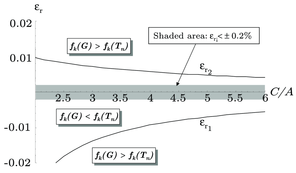
which define an interval $\left[\epsilon_{r_{1}},\epsilon_{r_{2}}\right]$ such that $f_{k}(G)\ll f_{k}(T_{n})$ for $\epsilon_{r_{1}}\ll\epsilon_{r}\ll\epsilon_{r_{2}}$ and $f_{k}(G)\gg f_{k}(T_{n})$ otherwise. From equation (3.2.2) it is apparent that the width of the interval $\left[\epsilon_{r_{1}},\epsilon_{r_{2}}\right]$ is smaller for the high frequency channels, characterised by higher values of the noise temperature; therefore the requirement on the gain modulation factor accuracy is determined by the 100 GHz channel.

Figure 4 shows the behaviour of $\epsilon_{r_{1}}$ and $\epsilon_{r_{2}}$ versus the ratio between gain and noise temperature fluctuations (i.e. $C/A=2\,\sqrt{N_{s}}$) for the 100 GHz channel. The region between the two curves corresponds to values of $\epsilon_{r}$ for which the noise temperature $1/f$ fluctuations dominate over gain instabilities. From the figure it is apparent that $1/f$ noise arising from gain fluctuations do not dominate if the gain modulation factor is accurate at the level of $\leq\pm\,0.2\,\%$.

Let us estimate the uncertainty in $r$ introduced by the largest expected fluctuation in the signal, i.e. the CMB dipole. If the fluctuation induced by the Dipole were larger than the requirement, then it would be necessary to calculate $r$ almost in real-time, in sub-minute time scales. From a simple calculation of $\delta r/r=\delta T_{\rm dipole}/\left(T_{x}+T_{n}\right)$ it follows that $\delta r/r\sim 10^{-4}$, which indicates that it will be possible to update $r$ on longer time-scales (of the order of few days) to account for variations caused by slow instrumental drifts.

Figure 4: Behaviour of $\epsilon_{r_{1}}$ and $\epsilon_{r_{2}}$ (calculated from equation (3.2.2)) as a function of $C/A$ for the 100 GHz channel. From the figure if follows that $f_{k}(G)<f_{k}(T_{n})$ (i.e. noise temperature fluctuations dominate) if the gain modulation factor is stable at the level of $\leq\pm\,0.2\,\%$.

Let us now analyse the effect of a small leakage across the first hybrid coupler, in the balanced radiometer approximation; if $\epsilon$ is the fraction of a signal applied to one port that shows up in the isolated port, then we can write the averaged power output, $\overline{p}$, as:

$$\overline{p}={ak\beta G}\left\{{T_{x}+T_{n}{(1+\epsilon)}^{2}-r\left[{T_{y}+T_{n}{(1-\epsilon)}^{2}}\right]}\right\}$$ (21)

The change in output caused by a small change in gain with the presence of such non-ideal isolation is:

$$\frac{\partial\overline{p}}{\partial G}={ak\beta}\left\{{T_{x}+T_{n}{(1+\epsilon)}^{2}-r\left[{T_{y}+T_{n}{(1-\epsilon)}^{2}}\right]}\right\}$$ (22)

Now, with the correct choice of $r$, we can make the sensitivity to gain fluctuations vanish and null the average output of the radiometer simultaneously:

$$r=\frac{T_{x}+T_{n}{(1+\epsilon)}^{2}}{T_{y}+T_{n}{(1-\epsilon)}^{2}}$$ (23)

Note that this freedom of choice for $r$ is not available to correlation radiometer designs without gain modulation, and therefore they are subject to $1/f$ fluctuations on the non-isolated fraction of the signal.

3.3 Sensitivity to back-end amplifier gain fluctuations

In this section we analyse the radiometer sensitivity to gain fluctuations of the back end amplifiers. Considering that the back-end noise is suppressed by a factor $\sim 10^{3}$ by the front-end amplification we can neglect the contribution of the noise temperature fluctuations.

Let us consider the case of a perfectly balanced front-end and suppose that the gain value in the two states of the phase switch is different by $\Delta G_{B}$.

The power output from a single radiometer leg will be then given by:

$$p=p_{x}-r\,p_{y}$$

$$p_{x}=a\,k\,\beta\,G_{F}\,G_{B}\left(T_{x}+T_{n_{F}}+T_{n_{B}}/G_{F}\right)$$ (24)

$$p_{y}=a\,k\,\beta\,G_{F}\,(G_{B}+\Delta G_{B})\left(T_{x}+T_{n_{F}}+T_{n_{B}}/G_{F}\right)$$

A straightforward analysis shows that the fluctuation $\Delta G_{B}$ will cause an equivalent spurious signal

$$\Delta T_{\rm eq}=-r\,\frac{\Delta G_{B}}{G_{B}}\left(T_{y}+T_{n_{F}}+T_{n_{B}}/G_{F}\right)$$ (25)

Substituting $\Delta G_{B}/G_{B}=C/\sqrt{f}$, $r=r^{*}_{0}$ and setting $\Delta T_{\rm equiv}$ equal to the single radiometer leg spectral density (equal to $2\,\beta^{-1/2}\left(T_{x}+T_{n_{tot}}\right)$, see equation (7)) we can calculate the post-detection knee-frequency as:

$$f_{k}^{0}(G_{B})=\beta\,N_{s}\,A^{2}$$ (26)

Using typical values for $\beta$, $N_{s}$ and $A$ in equation (26) it follows that the post-detection knee frequency arising from back-end gain fluctuations can be much greater than 1 Hz. Therefore to eliminate the contribution of the back-end $1/f$ noise we need a phase switch frequency such that $f_{\rm sw}\gg f_{k}^{0}(G_{B})$, so that the gain will be constant during the post-detection integration time.

For the LFI radiometers we have chosen a phase switch frequency of $\sim$ 4 KHz which leads to a small back-end $1/f$ contribution to the overall radiometer knee frequency for expected values of back-end gain fluctuations.

3.4 Sensitivity to reference load fluctuations

Proceeding as in the previous section we have that the signal mimicked by reference load fluctuations, $\Delta T_{y}$, is given by $\Delta T_{\rm eq}=-r\Delta T_{y}$.

If we consider random fluctuations in the reference load signal with a spectral density given by $\Delta T_{y}(f)$ then we have that these fluctuations equal the white noise for:

$$\Delta T_{y}(f)=\Delta T_{y}^{0}(f)\left[1+\frac{\alpha_{3}\,\epsilon_{T_{n}}}{4}-\left(r-\frac{1}{r}\right)\frac{\epsilon_{G}^{2}}{16}\right]$$ (27)

where $\Delta T_{y}^{0}(f)=\sqrt{2/\beta}\,(T_{y}+T_{n})$ and $\alpha_{3}$ is defined in equation (32).

This provides an upper limit to allowed random fluctuations in $T_{y}$ in order not to dominate the noise of the radiometer. For typical LFI parameters, this upper limit is of the order of $\Delta T_{y}\sim 1.8\times 10^{-4}{\rm K}/\sqrt{\rm Hz}$ at 30 GHz, slightly increasing for the higher frequency channels ($3.2\times 10^{-4}{\rm K}/\sqrt{\rm Hz}$ at 100 GHz). If we now consider the reference load in a global systematic error budget for LFI (the details of which are outside the scope of our paper) this implies requirements that are about one order of magnitude smaller than the above values.

If we consider non random fluctuations in the reference signal then the error induced by these variations must be much less than the sensitivity per pixel in the final maps. This error, that depends on the spectral behaviour of the spurious signal, on the satellite scanning strategy and on the data analysis procedures to build the sky maps, can be estimated using the approach described in Mennella et al. (mennella2002 (2002)). If we follow this approach considering that the parameter $r$ is of order unity, we have that spin synchronous variations of the reference signal will be transferred directly to the final maps, while slower fluctuations will be damped by a factor of the order of $10^{-2}$ - $10^{-3}$ by the measurement strategy and by data analysis.

4 Conclusions

In this paper we have discussed the pseudo-correlation architecture adopted for the radiometers of the Planck-LFI instrument and we have studied the sensitivity of the measured signal to various systematic effects. In our treatment we have considered both the ideal case of a perfectly balanced radiometer and the effect of small mismatches in the various radiometer parameters.

The first result is that the radiometer sensitivity does not depend on the level of the reference load temperature; even in the case of a slight imbalance in the radiometer parameters the dependence on $T_{y}$ is at the level of $\partial\Delta T/\partial T_{y}\sim 10^{-5}$ which is negligible. The only mismatch which has a first-order impact on $\Delta T$ is the noise temperature mismatch of the front-end amplifiers; our analysis shows that it is possible to maintain the sensitivity degradation below 1% with a noise temperature match better than 5%.

With proper gain modulation ($r=r^{*}_{0}$) the $1/f$ noise in the radiometer output is determined mainly by noise temperature fluctuations in the front-end amplifiers, with a knee frequency of few mHz, provided that the front-end amplifier amplitude match is better that $\sim\pm 0.5$ dB. Such a high level of $1/f$ noise suppression depends on the gain modulation factor, which must be determined with an accuracy better than $\pm 0.2\%$. If the accuracy on $r$ is less than $\pm 1\%$ then gain fluctuations become the major source of $1/f$ noise; if $\epsilon_{r}$ is kept in the range $\pm 1\%$ we expect values of the knee frequency of the order of 50 mHz which can be easily handled by destriping algorithms. The presence of a small amount of leakage in the first hybrid does not significantly modify this conclusion; with the correct choice of $r$, one can make the sensitivity to gain fluctuations vanish and null the average output of the radiometer simultaneously.

The effect of gain fluctuations in the back-end amplifiers can be made negligible by the fast front-end switching between sky and reference load signals. The LFI baseline of 4096 Hz for the phase switch frequency has been chosen to guarantee a high suppression level of the $1/f$ noise from back-end amplifiers.

In general our analysis demonstrates the effectiveness of the gain modulation concept applied to this form of radiometer. The estimate of the knee frequency given by equation (16) is quite low and relatively immune to small imperfections in radiometer balance. The modified correlation radiometer scheme reduces the knee frequency by more than two orders of magnitude, compared to a total power radiometer of similar bandwidth and intrinsic transistor fluctuations. For such small residual knee frequency (of $\sim 0.1$ Hz) it will be possible to remove efficiently the effects during data analysis.

We have also studied the sensitivity of the radimeter to changes in the reference load temperature, $T_{y}$. Our analysis provides a framework in which thermal stability requirements on the LFI reference loads can be evaluated.

A refinement of the present analysis for the determination of $f_{k}$ will be pursued in the future by software simulations of the radiometer functions to accurately study the combined effect of all components. Finally, laboratory measurements of a prototype radiometer working under conditions close to those of Planck mission constitute the most important checks for the ultimately understanding of the behaviour of Planck LFI radiometers regarding the $1/f$ type noise and possible further effects. Results of preliminary laboratory measurements performed of Planck-LFI prototype radiometers will be presented in forthcoming publications.

Appendix A Power output

The radiometer power output at each of the radiometer output legs is defined by:

$$p_{1}(t)= \frac{a}{4}\,g_{B_{1}}^{2}\,\left\{\left[\left(2\,n_{B_{1}}\cos{(\phi_{B_{1}})}+g_{F_{1}}(\sqrt{2}\,n_{F_{1}}+x+y)\cos{(\phi_{F_{1}}+\phi_{B_{1}})}+\right.\right.\right.$$ (28)

$$\,\,\,\,\,\,\,\,\,\,\,\,\,\,\,\,\,\,\,\,\,\,\,\,\left.+\sqrt{A_{1}}\,g_{F_{2}}(\sqrt{2}\,n_{F_{2}}+x-y)\cos{(\theta_{1}+\phi_{F_{2}}+\phi_{B_{1}})}\right)^{2}+$$

$$+\left(2\,n_{B_{1}}\sin{(\phi_{B_{1}})}+g_{F_{1}}(\sqrt{2}\,n_{F_{1}}+x+y)\sin{(\phi_{F_{1}}+\phi_{B_{1}})}+\right.$$

$$\,\,\,\,\,\,\,\,\,\,\,\,\,\,\,\,\,\,\,\,\,\,\,\,\left.\left.+\sqrt{A_{1}}\,g_{F_{2}}(\sqrt{2}\,n_{F_{2}}+x-y)\sin{(\theta_{1}+\phi_{F_{2}}+\phi_{B_{1}})}\right)^{2}\right]+$$

$$-r\,\left[\left(2\,n_{B_{1}}\cos{(\phi_{B_{1}})}+g_{F_{1}}(\sqrt{2}\,n_{F_{1}}+x+y)\cos{(\phi_{F_{1}}+\phi_{B_{1}})}+\right.\right.$$

$$\,\,\,\,\,\,\,\,\,\,\,\,\,\,\,\,\,\,\,\,\,\,\,\,\left.+\sqrt{A_{2}}\,g_{F_{2}}(\sqrt{2}\,n_{F_{2}}+x-y)\cos{(\theta_{2}+\phi_{F_{2}}+\phi_{B_{1}})}\right)^{2}+$$

$$+\left(2\,n_{B_{1}}\sin{(\phi_{B_{1}})}+g_{F_{1}}(\sqrt{2}\,n_{F_{1}}+x+y)\sin{(\phi_{F_{1}}+\phi_{B_{1}})}+\right.$$

$$\,\,\,\,\,\,\,\,\,\,\,\,\,\,\,\,\,\,\,\,\,\,\,\,\left.\left.\left.+\sqrt{A_{2}}\,g_{F_{2}}(\sqrt{2}\,n_{F_{2}}+x-y)\sin{(\theta_{2}+\phi_{F_{2}}+\phi_{B_{1}})}\right)^{2}\right]\right\}$$

where $a$ is the constant of proportionality of the square-law detectors. A similar relationship holds for $p_{2}(t)$.

Appendix B Sensitivity

B.1 Outline for sensitivity calculation

In this appendix we outline the procedure to calculate the LFI radiometer sensitivity (see equation (29)). We start from the expression of the power output $p(t)$, which is given by equation (28) and then we calculate the autocorrelation of $p(t)$, denoted as $\psi_{p}({\tau})\equiv\overline{p(t)p(t+\tau)}$. Note that we assume that $x$, $y$, $n_{1}$, and $n_{2}$ are all uncorrelated gaussian variables so that $\overline{xy}=\overline{x}\,\overline{y}$ and that they all have zero mean. The next step is the calculation of the Fourier transform of $\psi_{p}(\tau)$ (indicated by $Q_{p}(f)$, which can be split in a constant part, $Q_{p}(0)$, and in a fluctuating part $Q_{p}^{\prime}(f)$. Then we calculate the rms voltage $w_{\rm rms}={\overline{w(t)^{2}}}^{1/2}$ where $\overline{w(t)^{2}}=\int_{-\infty}^{+\infty}dfH(f)Q_{p}^{\prime}(f)$ and $H(f)$ is a rectangular lowpass filter of height $H_{0}$ and width $b$. The last step is to calculate the change in power output $\Delta p$ determined by a change in the sky signal equal to $\Delta T$; the sensitivity $\Delta T$ is then calculated by solving the equation $w_{\rm rms}=H_{0}^{1/2}\Delta p$.

B.2 Sensitivity analytical form

The radiometer sensitivity $\Delta T$ (calculated according to the procedure outlined above) has the following form:

$$\Delta T=\frac{1}{2}\left[\Delta{T_{1}^{2}}+\Delta{T_{2}^{2}}\right]^{\frac{1}{2}}$$ (29)

where $\Delta T_{1}$ and $\Delta T_{2}$ (which represent the minimum detectable rms signal on each single radiometer leg) are defined by the following equations:

$$\Delta{T_{1}}={\sqrt{\frac{1}{2\beta\tau}}}\frac{{\left(A-B\,r+C\,r^{2}\right)}^{\frac{1}{2}}}{\hat{G}-r\hat{I}}$$

$$\Delta{T_{2}}={\sqrt{\frac{1}{2\beta\tau}}}\frac{{\left(D-E\,r+F\,r^{2}\right)}^{\frac{1}{2}}}{\tilde{G}-r\tilde{I}}$$ (30)

The coefficients $A$ through $F$ have the following form:

$$A=a_{1}T_{x}^{2}+a_{2}T_{y}^{2}+a_{3}T_{x}+a_{4}T_{y}+a_{5}T_{x}T_{y}+a_{6}$$ (31)

with similar relationships for $B$, $C$, $D$, $E$ and $F$. Coefficients $a_{j}$, $b_{j}$, etc. are defined as follows:

B.2.1 Definitions of $a_{j}$ coefficients

$$a_{1}= 2\,\hat{G}^{2}$$

$$a_{2}= 2\,\tilde{I}^{2}$$

$$a_{3}= a_{31}\,T_{n_{F_{1}}}+a_{32}\,T_{n_{F_{2}}}+a_{33}\,T_{n_{B_{1}}}$$

$${a_{31}}=\frac{1}{2}\,{G_{F_{1}}}\,{\left[{\sqrt{{G_{F_{1}}}}}+{\sqrt{{A_{1}}\,{G_{F_{2}}}}}\,\cos({{\theta}_{1}}-{{\phi}_{F_{1}}}+{{\phi}_{F_{2}}})\right]}^{2}$$

$${a_{32}}=\frac{1}{2}\,{A_{1}}\,{G_{F_{2}}}\,{\left[{\sqrt{{A_{1}}\,{G_{F_{2}}}}}+{\sqrt{{G_{F_{1}}}}}\,\cos({{\theta}_{1}}-{{\phi}_{F_{1}}}+{{\phi}_{F_{2}}})\right]}^{2}$$

$${a_{33}}={\left[{\sqrt{{G_{F_{1}}}}}\,\cos({{\phi}_{F_{1}}})+{\sqrt{{A_{1}}\,{G_{F_{2}}}}}\,\cos({{\theta}_{1}}+{{\phi}_{F_{2}}})\right]}^{2}$$

$$a_{4}= a_{41}\,{T_{{n_{F_{1}}}}}+{a_{42}}\,{T_{{n_{2}}}}+{a_{43}}\,{T_{{n_{B_{1}}}}}$$

$${a_{41}}=\frac{1}{2}\,{G_{F_{1}}}\,{\left[{\sqrt{{G_{F_{1}}}}}-{\sqrt{{A_{1}}\,{G_{F_{2}}}}}\,\cos({{\theta}_{1}}-{{\phi}_{F_{1}}}+{{\phi}_{F_{2}}})\right]}^{2}$$

$${a_{42}}=\frac{1}{2}\,{A_{1}}\,{G_{F_{2}}}\,{\left[{\sqrt{{A_{1}}\,{G_{F_{2}}}}}-{\sqrt{{G_{F_{1}}}}}\,\cos({{\theta}_{1}}-{{\phi}_{F_{1}}}+{{\phi}_{F_{2}}})\right]}^{2}$$

$${a_{43}}={\left[{\sqrt{{G_{F_{1}}}}}\,\cos({{\phi}_{F_{1}}})-{\sqrt{{A_{1}}\,{G_{F_{2}}}}}\,\cos({{\theta}_{1}}+{{\phi}_{F_{2}}})\right]}^{2}$$

$${a_{5}}= \frac{1}{4}\,{\left({G_{F_{1}}}-{A_{1}}\,{G_{F_{2}}}\right)}^{2}$$

$${a_{6}}= \frac{1}{2}\,{G_{F_{1}}}\,{T_{{n_{F_{1}}}}}\,\left[{G_{F_{1}}}\,{T_{{n_{F_{1}}}}}+4\,{\cos({{\phi}_{F_{1}}})}^{2}\,{T_{{n_{B_{1}}}}}\right]+$$

$$+\frac{1}{2}\,{A_{1}}\,{G_{F_{2}}}\,{T_{{n_{F_{2}}}}}\,\left[2\,{\cos({{\theta}_{1}}-{{\phi}_{F_{1}}}+{{\phi}_{F_{2}}})}^{2}\,{G_{F_{1}}}\,{T_{{n_{F_{1}}}}}+{A_{1}}\,{G_{F_{2}}}\,{T_{{n_{2}}}}+4\,{\cos({{\theta}_{1}}+{{\phi}_{F_{2}}})}^{2}\,{T_{{n_{B_{1}}}}}\right]+2\,{{T_{{n_{B_{1}}}}^{2}}}$$

B.2.2 Definitions of $b_{j}$ coefficients

$$b_{1}= 4\,\hat{I}\,\hat{G}$$

$$b_{2}= 4\,\tilde{I}\,\tilde{G}$$

$$b_{3}= b_{31}\,T_{n_{F_{1}}}+b_{32}\,T_{n_{F_{2}}}+b_{33}\,T_{n_{B_{1}}}$$

$${b_{31}}={G_{F_{1}}}\,\left[{\sqrt{{G_{F_{1}}}}}+{\sqrt{{A_{1}}\,{G_{F_{2}}}}}\,\cos({{\theta}_{1}}-{{\phi}_{F_{1}}}+{{\phi}_{F_{2}}})\right]\,\left[{\sqrt{{G_{F_{1}}}}}+{\sqrt{{A_{2}}\,{G_{F_{2}}}}}\,\cos({{\theta}_{2}}-{{\phi}_{F_{1}}}+{{\phi}_{F_{2}}})\right]$$

$${b_{32}}={\sqrt{{A_{1}}\,{A_{2}}}}\,{G_{F_{2}}}\,\left[{\sqrt{{A_{1}}\,{G_{F_{2}}}}}+{\sqrt{{G_{F_{1}}}}}\,\cos({{\theta}_{1}}-{{\phi}_{F_{1}}}+{{\phi}_{F_{2}}})\right]\,\left[{\sqrt{{A_{2}}\,{G_{F_{2}}}}}+{\sqrt{{G_{F_{1}}}}}\,\cos({{\theta}_{2}}-{{\phi}_{F_{1}}}+{{\phi}_{F_{2}}})\right]$$

$${b_{33}}=2\,\left[{\sqrt{{G_{F_{1}}}}}\,\cos({{\phi}_{F_{1}}})+{\sqrt{{A_{1}}\,{G_{F_{2}}}}}\,\cos({{\theta}_{1}}+{{\phi}_{F_{2}}})\right]\,\left[{\sqrt{{G_{F_{1}}}}}\,\cos({{\phi}_{F_{1}}})+{\sqrt{{A_{2}}\,{G_{F_{2}}}}}\,\cos({{\theta}_{2}}+{{\phi}_{F_{2}}})\right]$$

$$b_{4}= b_{41}\,{T_{{n_{F_{1}}}}}+{b_{42}}\,{T_{{n_{F_{2}}}}}+{b_{43}}\,{T_{{n_{B_{1}}}}}$$

$${b_{41}}={G_{F_{1}}}\,\left[{\sqrt{{G_{F_{1}}}}}-{\sqrt{{A_{1}}\,{G_{F_{2}}}}}\,\cos({{\theta}_{1}}-{{\phi}_{F_{1}}}+{{\phi}_{F_{2}}})\right]\,\left[{\sqrt{{G_{F_{1}}}}}-{\sqrt{{A_{2}}\,{G_{F_{2}}}}}\,\cos({{\theta}_{2}}-{{\phi}_{F_{1}}}+{{\phi}_{F_{2}}})\right]$$

$${b_{42}}={\sqrt{{A_{1}}\,{A_{2}}}}\,{G_{F_{2}}}\,\left[{\sqrt{{A_{1}}\,{G_{F_{2}}}}}-{\sqrt{{G_{F_{1}}}}}\,\cos({{\theta}_{1}}-{{\phi}_{F_{1}}}+{{\phi}_{F_{2}}})\right]\,\left[{\sqrt{{A_{2}}\,{G_{F_{2}}}}}-{\sqrt{{G_{F_{1}}}}}\,\cos({{\theta}_{2}}-{{\phi}_{F_{1}}}+{{\phi}_{F_{2}}})\right]$$

$${b_{43}}=2\,\left[{\sqrt{{G_{F_{1}}}}}\,\cos({{\phi}_{F_{1}}})-{\sqrt{{A_{1}}\,{G_{F_{2}}}}}\,\cos({{\theta}_{1}}+{{\phi}_{F_{2}}})\right]\,\left[{\sqrt{{G_{F_{1}}}}}\,\cos({{\phi}_{F_{1}}})-{\sqrt{{A_{2}}\,{G_{F_{2}}}}}\,\cos({{\theta}_{2}}+{{\phi}_{F_{2}}})\right]$$

$${b_{5}}= \frac{1}{2}\,\left({G_{F_{1}}}-{A_{1}}\,{G_{F_{2}}}\right)\,\left({G_{F_{1}}}-{A_{2}}\,{G_{F_{2}}}\right)$$

$${b_{6}}= {G_{F_{1}}}\,{T_{{n_{F_{1}}}}}\,\left[{G_{F_{1}}}\,{T_{{n_{F_{1}}}}}+4\,{\cos({{\phi}_{F_{1}}})}^{2}\,{T_{{n_{B_{1}}}}}\right]+$$

$$+ {G_{F_{2}}}\,\sqrt{{A_{1}}\,{A_{2}}}{T_{{n_{F_{2}}}}}\,\left[\sqrt{{A_{1}}\,{A_{2}}}\,{G_{F_{2}}}\,{T_{{n_{F_{2}}}}}+4\,{T_{{n_{B_{1}}}}}\,\cos({{\theta}_{1}}+{{\phi}_{F_{2}}})\,\cos({{\theta}_{2}}+{{\phi}_{F_{2}}})+\right.$$

$$+ \left.2\,{G_{F_{1}}}\,{T_{{n_{F_{1}}}}}\,\cos({{\theta}_{1}}-{{\phi}_{F_{1}}}+{{\phi}_{F_{2}}})\,\cos({{\theta}_{2}}-{{\phi}_{F_{1}}}+{{\phi}_{F_{2}}})\right]+4\,{{T_{{n_{B_{1}}}}^{2}}}$$

B.2.3 Definitions of $c_{j}$ coefficients

$$c_{1}= 2\,\hat{I}^{2}$$

$$c_{2}= 2\,\tilde{G}^{2}$$

$$c_{3}= c_{31}\,T_{n_{F_{1}}}+c_{32}\,T_{n_{F_{2}}}+c_{33}\,T_{n_{B_{1}}}$$

$${c_{31}}=\frac{1}{2}\,{G_{F_{1}}}\,{\left[{\sqrt{{G_{F_{1}}}}}+{\sqrt{{A_{2}}\,{G_{F_{2}}}}}\,\cos({{\theta}_{2}}-{{\phi}_{F_{1}}}+{{\phi}_{F_{2}}})\right]}^{2}$$

$${c_{32}}=\frac{1}{2}\,{A_{2}}\,{G_{F_{2}}}\,{\left[{\sqrt{{A_{2}}\,{G_{F_{2}}}}}+{\sqrt{{G_{F_{1}}}}}\,\cos({{\theta}_{2}}-{{\phi}_{F_{1}}}+{{\phi}_{F_{2}}})\right]}^{2}$$

$${c_{33}}={\left[{\sqrt{{G_{F_{1}}}}}\,\cos({{\phi}_{F_{1}}})+{\sqrt{{A_{2}}\,{G_{F_{2}}}}}\,\cos({{\theta}_{2}}+{{\phi}_{F_{2}}})\right]}^{2}$$

$$c_{4}= c_{41}\,{T_{{n_{F_{1}}}}}+{c_{42}}\,{T_{{n_{F_{2}}}}}+{c_{43}}\,{T_{{n_{B_{1}}}}}$$

$${c_{41}}=\frac{1}{2}\,{G_{F_{1}}}\,{\left[{\sqrt{{G_{F_{1}}}}}-{\sqrt{{A_{2}}\,{G_{F_{2}}}}}\,\cos({{\theta}_{2}}-{{\phi}_{F_{1}}}+{{\phi}_{F_{2}}})\right]}^{2}$$

$${c_{42}}=\frac{1}{2}\,{A_{2}}\,{G_{F_{2}}}\,{\left[{\sqrt{{A_{2}}\,{G_{F_{2}}}}}-{\sqrt{{G_{F_{1}}}}}\,\cos({{\theta}_{2}}-{{\phi}_{F_{1}}}+{{\phi}_{F_{2}}})\right]}^{2}$$

$${c_{43}}={\left[{\sqrt{{G_{F_{1}}}}}\,\cos({{\phi}_{F_{1}}})-{\sqrt{{A_{2}}\,{G_{F_{2}}}}}\,\cos({{\theta}_{2}}+{{\phi}_{F_{2}}})\right]}^{2}$$

$${c_{5}}= \frac{1}{4}\,{\left({G_{F_{1}}}-{A_{2}}\,{G_{F_{2}}}\right)}^{2}$$

$${c_{6}}= \frac{1}{2}\,{G_{F_{1}}}\,{T_{{n_{F_{1}}}}}\,\left[{G_{F_{1}}}\,{T_{{n_{F_{1}}}}}+4\,{\cos({{\phi}_{F_{1}}})}^{2}\,{T_{{n_{B_{1}}}}}\right]+$$

$$+\frac{1}{2}\,{A_{2}}\,{G_{F_{2}}}\,{T_{{n_{F_{2}}}}}\,\left[2\,{\cos({{\theta}_{2}}-{{\phi}_{F_{1}}}+{{\phi}_{F_{2}}})}^{2}\,{G_{F_{1}}}\,{T_{{n_{F_{1}}}}}+{A_{2}}\,{G_{F_{2}}}\,{T_{{n_{F_{2}}}}}+4\,{\cos({{\theta}_{2}}+{{\phi}_{F_{2}}})}^{2}\,{T_{{n_{B_{1}}}}}\right]+2\,{{T_{{n_{B_{1}}}}^{2}}}$$

B.2.4 Definitions of $d_{j}$ coefficients

$$d_{1}= 2\,\tilde{G}^{2}$$

$$d_{2}= 2\,\hat{I}^{2}$$

$$d_{3}= d_{3,1}\,T_{n_{F_{1}}}+d_{3,2}\,T_{n_{F_{2}}}+d_{3,3}\,T_{n_{B_{2}}}$$

$${d_{3,1}}=\frac{1}{2}\,{G_{F_{1}}}\,{\left[{\sqrt{{G_{F_{1}}}}}-{\sqrt{{A_{2}}\,{G_{F_{2}}}}}\,\cos({{\theta}_{2}}-{{\phi}_{F_{1}}}+{{\phi}_{F_{2}}})\right]}^{2}$$

$${d_{3,2}}=\frac{1}{2}\,{A_{2}}\,{G_{F_{2}}}\,{\left[{\sqrt{{A_{2}}\,{G_{F_{2}}}}}-{\sqrt{{G_{F_{1}}}}}\,\cos({{\theta}_{2}}-{{\phi}_{F_{1}}}+{{\phi}_{F_{2}}})\right]}^{2}$$

$${d_{3,3}}={\left[{\sqrt{{G_{F_{1}}}}}\,\cos({{\phi}_{F_{1}}})-{\sqrt{{A_{2}}\,{G_{F_{2}}}}}\,\cos({{\theta}_{2}}+{{\phi}_{F_{2}}})\right]}^{2}$$

$$d_{4}= d_{4,1}\,{T_{{n_{F_{1}}}}}+{d_{4,2}}\,{T_{{n_{F_{2}}}}}+{d_{4,3}}\,{T_{{n_{B_{2}}}}}$$

$${d_{4,1}}=\frac{1}{2}\,{G_{F_{1}}}\,{\left[{\sqrt{{G_{F_{1}}}}}+{\sqrt{{A_{2}}\,{G_{F_{2}}}}}\,\cos({{\theta}_{2}}-{{\phi}_{F_{1}}}+{{\phi}_{F_{2}}})\right]}^{2}$$

$${d_{4,2}}=\frac{1}{2}\,{A_{2}}\,{G_{F_{2}}}\,{\left[{\sqrt{{A_{2}}\,{G_{F_{2}}}}}+{\sqrt{{G_{F_{1}}}}}\,\cos({{\theta}_{2}}-{{\phi}_{F_{1}}}+{{\phi}_{F_{2}}})\right]}^{2}$$

$${d_{4,3}}={\left[{\sqrt{{G_{F_{1}}}}}\,\cos({{\phi}_{F_{1}}})+{\sqrt{{A_{2}}\,{G_{F_{2}}}}}\,\cos({{\theta}_{2}}+{{\phi}_{F_{2}}})\right]}^{2}$$

$${d_{5}}= \frac{1}{4}\,{\left({G_{F_{1}}}-{A_{2}}\,{G_{F_{2}}}\right)}^{2}$$

$${d_{6}}= \frac{1}{2}\,{G_{F_{1}}}\,{T_{{n_{F_{1}}}}}\,\left[{G_{F_{1}}}\,{T_{{n_{F_{1}}}}}+4\,{\cos({{\phi}_{F_{1}}})}^{2}\,{T_{{n_{B_{2}}}}}\right]+$$

$$+\frac{1}{2}\,{A_{2}}\,{G_{F_{2}}}\,{T_{{n_{F_{2}}}}}\,\left[2\,{\cos({{\theta}_{2}}-{{\phi}_{F_{1}}}+{{\phi}_{F_{2}}})}^{2}\,{G_{F_{1}}}\,{T_{{n_{F_{1}}}}}+{A_{2}}\,{G_{F_{2}}}\,{T_{{n_{F_{2}}}}}+4\,{\cos({{\theta}_{2}}+{{\phi}_{F_{2}}})}^{2}\,{T_{{n_{B_{2}}}}}\right]+2\,{{T_{{n_{B_{2}}}}^{2}}}$$

B.2.5 Definitions of $e_{j}$ coefficients

$$e_{1}= 4\,\tilde{I}\,\tilde{G}$$

$$e_{2}= 4\,\hat{I}\,\hat{G}$$

$$e_{3}= d_{3,1}\,T_{n_{F_{1}}}+d_{3,2}\,T_{n_{F_{2}}}+d_{3,3}\,T_{n_{B_{2}}}$$

$${e_{3,1}}={G_{F_{1}}}\,\left[{\sqrt{{G_{F_{1}}}}}-{\sqrt{{A_{1}}\,{G_{F_{2}}}}}\,\cos({{\theta}_{1}}-{{\phi}_{F_{1}}}+{{\phi}_{F_{2}}})\right]\,\left[{\sqrt{{G_{F_{1}}}}}-{\sqrt{{A_{2}}\,{G_{F_{2}}}}}\,\cos({{\theta}_{2}}-{{\phi}_{F_{1}}}+{{\phi}_{F_{2}}})\right]$$

$${e_{3,2}}={\sqrt{{A_{1}}\,{A_{2}}}}\,{G_{F_{2}}}\,\left[{\sqrt{{A_{1}}\,{G_{F_{2}}}}}-{\sqrt{{G_{F_{1}}}}}\,\cos({{\theta}_{1}}-{{\phi}_{F_{1}}}+{{\phi}_{F_{2}}})\right]\,\left[{\sqrt{{A_{2}}\,{G_{F_{2}}}}}-{\sqrt{{G_{F_{1}}}}}\,\cos({{\theta}_{2}}-{{\phi}_{F_{1}}}+{{\phi}_{F_{2}}})\right]$$

$${e_{3,3}}=2\,\left[{\sqrt{{G_{F_{1}}}}}\,\cos({{\phi}_{F_{1}}})-{\sqrt{{A_{1}}\,{G_{F_{2}}}}}\,\cos({{\theta}_{1}}+{{\phi}_{F_{2}}})\right]\,\left[{\sqrt{{G_{F_{1}}}}}\,\cos({{\phi}_{F_{1}}})-{\sqrt{{A_{2}}\,{G_{F_{2}}}}}\,\cos({{\theta}_{2}}+{{\phi}_{F_{2}}})\right]$$

$$e_{4}= e_{4,1}\,{T_{{n_{F_{1}}}}}+{e_{4,2}}\,{T_{{n_{F_{2}}}}}+{e_{4,3}}\,{T_{{n_{B_{2}}}}}$$

$${e_{4,1}}={G_{F_{1}}}\,\left[{\sqrt{{G_{F_{1}}}}}+{\sqrt{{A_{1}}\,{G_{F_{2}}}}}\,\cos({{\theta}_{1}}-{{\phi}_{F_{1}}}+{{\phi}_{F_{2}}})\right]\,\left[{\sqrt{{G_{F_{1}}}}}+{\sqrt{{A_{2}}\,{G_{F_{2}}}}}\,\cos({{\theta}_{2}}-{{\phi}_{F_{1}}}+{{\phi}_{F_{2}}})\right]$$

$${e_{4,2}}={\sqrt{{A_{1}}\,{A_{2}}}}\,{G_{F_{2}}}\,\left[{\sqrt{{A_{1}}\,{G_{F_{2}}}}}+{\sqrt{{G_{F_{1}}}}}\,\cos({{\theta}_{1}}-{{\phi}_{F_{1}}}+{{\phi}_{F_{2}}})\right]\,\left[{\sqrt{{A_{2}}\,{G_{F_{2}}}}}+{\sqrt{{G_{F_{1}}}}}\,\cos({{\theta}_{2}}-{{\phi}_{F_{1}}}+{{\phi}_{F_{2}}})\right]$$

$${e_{4,3}}=2\,\left[{\sqrt{{G_{F_{1}}}}}\,\cos({{\phi}_{F_{1}}})+{\sqrt{{A_{1}}\,{G_{F_{2}}}}}\,\cos({{\theta}_{1}}+{{\phi}_{F_{2}}})\right]\,\left[{\sqrt{{G_{F_{1}}}}}\,\cos({{\phi}_{F_{1}}})+{\sqrt{{A_{2}}\,{G_{F_{2}}}}}\,\cos({{\theta}_{2}}+{{\phi}_{F_{2}}})\right]$$

$${e_{5}}= \frac{1}{2}\,\left({G_{F_{1}}}-{A_{1}}\,{G_{F_{2}}}\right)\,\left({G_{F_{1}}}-{A_{2}}\,{G_{F_{2}}}\right)$$

$${e_{6}}= {G_{F_{1}}}\,{T_{{n_{F_{1}}}}}\,\left[{G_{F_{1}}}\,{T_{{n_{F_{1}}}}}+4\,{\cos({{\phi}_{F_{1}}})}^{2}\,{T_{{n_{B_{2}}}}}\right]+$$

$$+ {G_{F_{2}}}\,\sqrt{{A_{1}}\,{A_{2}}}{T_{{n_{F_{2}}}}}\,\left[\sqrt{{A_{1}}\,{A_{2}}}\,{G_{F_{2}}}\,{T_{{n_{F_{2}}}}}+4\,{T_{{n_{B_{2}}}}}\,\cos({{\theta}_{1}}+{{\phi}_{F_{2}}})\,\cos({{\theta}_{2}}+{{\phi}_{F_{2}}})+\right.$$

$$+ \left.2\,{G_{F_{1}}}\,{T_{{n_{F_{1}}}}}\,\cos({{\theta}_{1}}-{{\phi}_{F_{1}}}+{{\phi}_{F_{2}}})\,\cos({{\theta}_{2}}-{{\phi}_{F_{1}}}+{{\phi}_{F_{2}}})\right]+4\,{{T_{{n_{B_{2}}^{2}}}}}$$

B.2.6 Definitions of $f_{j}$ coefficients

$$f_{1}= 2\,\tilde{I}^{2}$$

$$f_{2}= 2\,\hat{G}^{2}$$

$$f_{3}= f_{3,1}\,T_{n_{F_{1}}}+f_{3,2}\,T_{n_{F_{2}}}+f_{3,3}\,T_{n_{B_{2}}}$$

$${f_{3,1}}=\frac{1}{2}\,{G_{F_{1}}}\,{\left[{\sqrt{{G_{F_{1}}}}}-{\sqrt{{A_{1}}\,{G_{F_{2}}}}}\,\cos({{\theta}_{1}}-{{\phi}_{F_{1}}}+{{\phi}_{F_{2}}})\right]}^{2}$$

$${f_{3,2}}=\frac{1}{2}\,{A_{1}}\,{G_{F_{2}}}\,{\left[{\sqrt{{A_{1}}\,{G_{F_{2}}}}}-{\sqrt{{G_{F_{1}}}}}\,\cos({{\theta}_{1}}-{{\phi}_{F_{1}}}+{{\phi}_{F_{2}}})\right]}^{2}$$

$${f_{3,3}}={\left[{\sqrt{{G_{F_{1}}}}}\,\cos({{\phi}_{F_{1}}})-{\sqrt{{A_{1}}\,{G_{F_{2}}}}}\,\cos({{\theta}_{1}}+{{\phi}_{F_{2}}})\right]}^{2}$$

$$f_{4}= f_{4,1}\,{T_{{n_{F_{1}}}}}+{f_{4,2}}\,{T_{{n_{F_{2}}}}}+{f_{4,3}}\,{T_{{n_{B_{2}}}}}$$

$${f_{4,1}}=\frac{1}{2}\,{G_{F_{1}}}\,{\left[{\sqrt{{G_{F_{1}}}}}+{\sqrt{{A_{1}}\,{G_{F_{2}}}}}\,\cos({{\theta}_{1}}-{{\phi}_{F_{1}}}+{{\phi}_{F_{2}}})\right]}^{2}$$

$${f_{4,2}}=\frac{1}{2}\,{A_{1}}\,{G_{F_{2}}}\,{\left[{\sqrt{{A_{1}}\,{G_{F_{2}}}}}+{\sqrt{{G_{F_{1}}}}}\,\cos({{\theta}_{1}}-{{\phi}_{F_{1}}}+{{\phi}_{F_{2}}})\right]}^{2}$$

$${f_{4,3}}={\left[{\sqrt{{G_{F_{1}}}}}\,\cos({{\phi}_{F_{1}}})+{\sqrt{{A_{1}}\,{G_{F_{2}}}}}\,\cos({{\theta}_{1}}+{{\phi}_{F_{2}}})\right]}^{2}$$

$${f_{5}}= \frac{1}{4}\,{\left({G_{F_{1}}}-{A_{1}}\,{G_{F_{2}}}\right)}^{2}$$

$${f_{6}}= \frac{1}{2}\,{G_{F_{1}}}\,{T_{{n_{F_{1}}}}}\,\left[{G_{F_{1}}}\,{T_{{n_{F_{1}}}}}+4\,{\cos({{\phi}_{F_{1}}})}^{2}\,{T_{{n_{B_{2}}}}}\right]+$$

$$+\frac{1}{2}\,{A_{1}}\,{G_{F_{2}}}\,{T_{{n_{F_{2}}}}}\,\left[2\,{\cos({{\theta}_{1}}-{{\phi}_{F_{1}}}+{{\phi}_{F_{2}}})}^{2}\,{G_{F_{1}}}\,{T_{{n_{F_{1}}}}}+{A_{1}}\,{G_{F_{2}}}\,{T_{{n_{F_{2}}}}}+4\,{\cos({{\theta}_{1}}+{{\phi}_{F_{2}}})}^{2}\,{T_{{n_{B_{2}}}}}\right]+2\,{{T_{{n_{B_{2}}}}^{2}}}$$

Appendix C Definition of $\alpha$ parameters

The parameters $\alpha_{1}$ through $\alpha_{4}$ used in equations (2.2.3), (15), (16) and (27) are defined as:

$${{\alpha}_{1}}=\frac{(1+r)({T_{x}}-{T_{y}})}{8\left[{T_{x}}+{T_{n}}-r\,\left({T_{n}}+{T_{n}}\right)\right]}$$

$${{\alpha}_{2}}=\frac{\left(1-r\right)\,{T_{n}}}{{T_{x}}+{T_{n}}-r\,\left({T_{n}}+{T_{n}}\right)}$$

$${{\alpha}_{3}}={T_{n}}\,\left(\frac{1}{{T_{x}}+{T_{n}}}+\frac{1}{{T_{y}}+{T_{n}}}\right)$$

$${{\alpha}_{4}}=\frac{T_{x}-T_{y}}{{T_{y}}+{T_{n}}}$$ (32)

References

- (1) Bennett, C. L., et al., Astrophys. J. Lett., 464, L1, (1996)
- (2) Bersanelli, M., Mandolesi, N., Weinreb, S., Ambrosini, R., & Smoot, G. F., Int. Rep. ITeSRE 177/1995, March, (1995)
- (3) Bersanelli, M., et al., COBRAS/SAMBA Report on the Phase A Study, ESA D/SCI(96)3, (1996)
- (4) Bersanelli, M., Mennella, A., Burigana, C., Mandolesi, N., Technical Note, PL-LFI-PST-TN-033, (2002)
- (5) Blum, E. J., Annales d’Astrophysique, 22-2, 140, (1959)
- (6) Burigana, C., Malaspina, M., Mandolesi, N., et al., Int. Rep. TeSRE/CNR 198/1997, November, (1997), astro-ph/9906360
- (7) Burigana, C., Seiffert, M., Mandolesi, N., & Bersanelli, M., Int. Rep. TeSRE/CNR 186/1997, March, (1997)
- (8) Colvin, R. S., Ph.D. thesis, Stanford University, (1961)
- (9) Delabrouille, J., A&AS, 127, 555, (1998)
- (10) De Zotti, G., Toffolatti, L., Argüeso Gómez,, F., et al., Proceedings of the EC-TMR Conference “3 K Cosmology”, Roma, Italy, 5-10 October 1998, AIP Conference Proc. 476, Maiani L., Melchiorri F., Vittorio N., (Eds.), pg. 204, (1999), astro-ph/9902103
- (11) Doré, O., Teyssier, R., Bouchet, F. R., Vibert, D., & Prunet, S., A&A, 374, 358, (2001)
- (12) Hu, W., Sugiyama, N., & Silk, J., Nature, 386, 37, (1997)
- (13) Janssen, M. A., Scott, D., White, M., et al., (1996), astro-ph/9602009
- (14) Jarosik, N. C., IEEE Trans. Microwave Theory Tech., 44, 193, (1996)
- (15) Lubin, P., Meinhold, P., Childers, J., Astroph. Lett. Comm., 37, 205, (2000)
- (16) Maino, D., Burigana, C., Maltoni, M., et al., A&AS, 140, 383, (1999)
- (17) Maino, D., Burigana, C., Bersanelli, M., Mandolesi, N., & Pasian, F., Technical Note, PL-LFI-OAT-TN-014, (2000)
- (18) Mandolesi, N., et al., Planck LFI, A Proposal Submitted to the ESA, (1998)
- (19) Mennella, A., et al., A&A, 384, 736-742, (2002)
- (20) Natoli, P., de Gasperis, G., Gheller, C., & Vittorio, N., A&A, 372, 346, (2001)
- (21) Pospieszalski, IEEE Trans. Microwave Theory Tech, 37, 1340, (1989)
- (22) Puget, J. L., et al., HFI for the Planck Mission, A Proposal Submitted to the ESA, (1998)
- (23) Scott, D., Silk, J., & White, M., Science, 268, 829, (1995)
- (24) Smoot, G. F., et al. 1992, ApJ, 396, L1
- (25) White, M., Scott, D., and Silk, J., Ann. Rev. of Astron. and Astrophys., 32, 319, (1994)
- (26) Wollack, E. J., Rev. Sci. Instrum., 66, 4305, (1995)