Testing Stellar Population Models with Star Clusters in the Large Magellanic Cloud

Abstract

We present high signal-to-noise integrated spectra of 24 star clusters in the Large Magellanic Cloud (LMC), obtained using the FLAIR spectrograph at the UK Schmidt telescope. The spectra have been placed onto the Lick/IDS system in order to test the calibration of Simple Stellar Population (SSP) models (Maraston & Thomas 2000; Kurth, Fritz-von Alvensleben & Fricke 1999).

We have compared the SSP-predicted metallicities of the clusters with those from the literature, predominantly taken from the Ca-Triplet spectroscopy of Olszewski et al. (1991). We find that there is good agreement between the metallicities in the range –2.10 $\leq$ [Fe/H] $\leq$ 0. However, the Mg₂ index (and to a lesser degree Mg $b$) systematically predict higher metallicities (up to +0.5 dex higher) than $\langle$Fe$\rangle$. Among the possible explanations for this are that the LMC clusters possess [$\alpha$/Fe] $>$ 0. Metallicities are presented for eleven LMC clusters which have no previous measurements.

We compare SSP ages for the clusters, derived from the H$\beta$, H$\gamma$ and H$\delta$ Lick/IDS indices, with the available literature data, and find good agreement for the vast majority. This includes six old globular clusters in our sample, which have ages consistent with their HST CMD ages and/or integrated colours. However, two globular clusters, NGC 1754 and NGC 2005, identified as old ($\sim$ 15 Gyr) on the basis of HST CMDs, have H$\beta$ line-strengths which lead ages which are too young ($\sim$ 8 and $\sim$ 6 Gyr respectively). These findings are inconsistent with their CMD-derived values at the 3$\sigma$ level. Comparison between the horizontal branch morphology and the Balmer line-strengths of these clusters suggests that the presence of blue horizontal branch stars has increased their Balmer indices by up to $\sim$ 1.0 Å.

We conclude that the Lick/IDS indices, used in conjunction with contemporary SSP models, are able to reproduce the ages and metallicities of the LMC clusters reassuringly well. The required extrapolations of the fitting-functions and stellar libraries in the models to younger ages and low metallicities do not lead to serious systematic errors. However, due to the significant contribution of horizontal branch stars to Balmer indices, SSP model ages derived for metal-poor globular clusters are ambiguous without a priori knowledge of horizontal branch morphology.

1 Introduction

One of the most powerful tools available to observers of stellar populations is the colour-magnitude diagram (CMD). Whilst there still remain numerous uncertainties in stellar evolution theory (e.g. [Castellani et al. (2001)] 2001), the existence of accurate paralaxes such as those from HIPPARCOS, used in conjunction with contemporary model isochrones can now constrain the ages of Galactic globular clusters (GCs) to within $\sim$ 20% (e.g. [Carretta et al. (2000)] 2000).

Furthermore, HST has allowed us to obtain detailed information for GCs and field stars in external galaxies such as the LMC (e.g. [Holtzman et al. (1997)] 1997; [Olsen et al. (1998)] 1998; [Johnson et al. (1999)] 1999), the Andromeda galaxy (e.g. [Holland et al. (1996)] 1996; [Fusi Pecci et al. (1996)] 1996) and even the nearest large elliptical Centaurus A (e.g. [Soria et al. (1996)] 1996; [Harris et al. (1998)] 1998; [Harris et al. (1999)] 1999; [Marleau et al. (2000)] 2000).

However, such observations are challenging, and beyond several Mpc exceed the capabilities of current instrumentation. Even with HST, a combination of crowding and the intrinsic faintness of single stars limits the applicability of such an approach. Therefore, in order to probe the properties of distant stellar systems, we must rely upon studies of integrated light.

Integrated spectroscopy and photometry require comparisons with stellar population models, and are affected by a degeneracy between age and metallicity ([Faber (1972)] 1972; [O’Connell (1976)] 1976). Spectroscopic indices have been shown to hold potential, and much work in the past decade has lead to age-metallicity diagnostics for integrated spectra (e.g. Gonz$\acute{a}$lez 1993; [Rose (1994)] 1994; [Worthey (1994)] 1994; [Borges et al. (1995)] 1995; [Idiart & Pacheco (1995)] 1995; [Worthey & Ottaviani (1997)] 1997; [Vazdekis & Arimoto (1999)] 1999). These methods have subsequently been used by many workers to derive ages and metallicities for galaxies (e.g. [Davies et al. (1993)] 1993; Gonz$\acute{a}$lez 1993; [Fisher et al. (1995)] 1995; [Kuntschner & Davies (1998)] 1998; [Vazdekis et al. (2001a)] 2001) and extragalactic globular clusters (e.g. [Cohen et al. (1998)] 1998; [Kissler-Patig et al. (1998)] 1998; [Beasley et al. (2000)] 2000; [Forbes et al. (2001)] 2001).

However, the reliability of such integrated techniques has yet to be demonstrated: they must be tested against stellar systems with independently derived age and metallicity estimates such as Galactic GCs. Addressing this issue, [Gibson et al. (1999)] (1999) derived a ’spectroscopic’ age for 47 Tucanae in the H$\gamma_{\rm HR}$ – Fe4668 and H$\gamma_{\rm HR}$ – CaI_HR planes of the [Worthey (1994)] (1994; henceforth W94) simple stellar population (SSP) models. These authors found that 47 Tuc’s integrated spectrum fell below the oldest (17 Gyr) isochrones of the W94 models at the 4$\sigma$ level, yielding an extrapolated age in excess of 20 Gyr. By comparison, the CMD-derived age of 47 Tuc is 14 $\pm$ 1 Gyr [Richer et al. (1996)]. On the other hand, [Maraston & Thomas (2000)] (2000) derived an age of 15 Gyrs for this cluster using the combination H$\beta$ and Fe5335, in good agreement with the CMD of [Richer et al. (1996)] (1996). [Vazdekis et al. (2001b)] (2001) and [(68)] (2002) have recently addressed these issues and conclude that the inclusion of atomic diffusion and non-solar abundance ratios are important. Moreover, [(68)] (2002) found it necessary to include both AGB stars and adjust the metallicity of 47 Tuc by –0.05 dex to fit their SSP models to the integrated spectrum of this cluster.

Whilst these developments are extremely promising, the full calibration of SSP models has yet to be comprehensively tested. The Galactic GC 47 Tuc represents a single age and single metallicity in the large parameter space of contemporary SSP models. In view of the adjustments employed Schiavon et al. 2001 in order to reproduce the integrated spectrum of just this cluster, begs the question of how well can these models be applied to more distant, less well-known stellar systems? Furthermore, 47 Tuc is an idealised case of an old, relatively metal-rich stellar system which has a ’red clump’ for its horizontal branch (HB). In this case, the strength of the Balmer lines are thought to be primarily a function of the temperature of the main sequence turn-off (and hence age). At lower metallicities GCs develop blue HBs which are expected to contribute a significant component to Balmer lines (e.g. [Buzzoni (1989)] 1989; [de Freitas Pacheco & Barbuy (1995)] 1995; [Lee et al. (2000)] 2000; [Maraston & Thomas (2000)] 2000).

On the observational side, obtaining integrated spectra of Galactic GCs may hide other uncertainties. Owing to the large angular size of Galactic GCs on the sky (the half-light radius of 47 Tuc is $\sim$ 2.8 ^′) a spectroscopic aperture must be synthesised by physically scanning a slit across the cluster. In so doing, the observer may unwittingly include foreground stars in the integrated spectrum, in addition to increasing the liklihood of stochastic contributions from bright stars. Clearly, alternative laboratories are desirable to test SSP models.

The Large Magellanic Cloud (LMC) presents an ideal target for such tests. Many of its $\sim$ 2000 star clusters [Olszewski et al. (1996)] have been independently age-dated and their metallicities determined, whilst its proximity ($\sim$ 53  kpc) means that acquiring high S/N, integrated spectra of the clusters is relatively straightforward (e.g. [Rabin (1982)] 1982).

In this paper, we present high S/N integrated spectra for 24 star clusters in the LMC, covering a wide range in age (0.5 – 17 Gyr) and metallicity (–2.1 $\leq$ [Fe/H] $\leq$ 0). We have placed the clusters onto the Lick/IDS system and measured their line-strength indices in order to test contemporary stellar population models which use the Lick/IDS fitting-functions ([Gorgas et al. (1993)] 1993; [Worthey et al. (1994)] 1994; [Worthey & Ottaviani (1997)] 1997).

The plan of this paper is as follows: In Section 2, we describe our sample selection and the observations performed for this present study. In Section 3 we describe the reduction steps required for our fibre spectra. We discuss the spectroscopic system and the stellar population models we use in this study in Section 4. In Section 5, we derive ages and metallicities for the LMC clusters using the SSP models, which we then compare to literature values. Finally, we present our conclusions and a summary in Section 6.

2 Sample Selection and Observations

2.1 Star Clusters in the LMC

[Searle et al. (1980)] (1980; henceforth SWB) devised a one-dimensional classification scheme for LMC star clusters using integrated Gunn-Thuan photometry, and showed that the clusters primarily form an age sequence in the Q(ugr)-Q(vgr) diagram, with metallicity becoming increasingly important for the oldest clusters. SWB assigned ’SWB-types’ I–VII to the clusters, with I representing young, blue clusters through to VII, old and metal-poor clusters—essentially analogues of Milky Way GCs.

Subsequently, [Frenk & Fall (1982)] (1982) showed that the same sequence was apparent in the ’equivalent’ (U-B) vs (B-V) diagram, which they termed ’E-SWB’. [Elson & Fall (1985)] (1985) and [Elson & Fall (1988)] (1988) determined an age calibration for these SWB types by using literature age estimates, determined from either CMDs, integrated spectra, or from the extent of their asymptotic giant branches (e.g. [Mould & Aaronson (1982)] (1982). In this paper, we employ SWB-types to segregate the LMC clusters into age/metallicity groups for our analysis, using the revised age calibration given in [Bica et al. (1992)] (1992).

Our spectroscopic sample was selected on the basis of the availability of independent age and metallicity estimates for the clusters, SWB type and concentration. This final criterion was important so that we were able to match the core radii of the clusters to the size of the 6^′′ fibres of the FLAIR spectrograph (see below), thereby minimising background contamination. We took particular care to include SWB VII (globular) clusters in our sample, which have HST CMDs. Integrated colours, magnitudes and positions for our cluster sample were drawn from the catalogue of [Bica et al. (1999)] (1999), with SWB-types obtained from the earlier catalogue of [Bica et al. (1996)] (1996).

Our total spectroscopic sample comprised of SWB I–VII clusters. However, for the purposes of this analysis, only the clusters of type IVA ($\sim$ 0.4 Gyr) and older will be considered further, since the Lick/IDS fitting-functions were only calculated for ages of 0.5 Gyr and older (see [Worthey et al. (1994)] 1994). We list the 24 clusters in our sample for which we have obtained useful spectra in Table 2, along with their basic physical parameters. In addition, we give heliocentric radial velocities for the clusters obtained from cross-correlation against template stars. Although the resolution of our spectra is too low for accurate radial velocities, an approximate velocity is required in order to shift the spectra to the rest-frame for the measurement of line-strength indices. We have achieved S/N ratios of 66 – 340 Å^-1, calculated in the 5000Å region of the spectra (note that for the older clusters transmitted flux at the H$\gamma$ feature is typically a factor of $\sim$ 2 lower than at 5000Å, i.e. a factor of $\sqrt{2}$ lower in S/N.)

Table 2: Data for our observed star clusters. Columns are : (1) ID (2) heliocentric velocity, (3) velocity error, (4) right ascension, (5) declination, (6) apparent diameter, (7) integrated V magnitude, (8) $U-B$ colour, (9) $B-V$ colour, (10) SWB type, (11) signal to noise ratio. Sources: ¹ this work, ² from [Bica et al. (1999)] (1999) ,³ from [Bica et al. (1996)] (1996)

ID	V${}_{h}^{1}$	V${}_{err}^{1}$	RA(2000.0)2	DEC(2000.0)2	D 2	${\emph{V}}^{3}$	$U-B^{3}$	$B-V^{3}$	SWB type3	S/N1
	$\,\hbox{km}\,\hbox{s}^{-1}$	$\,\hbox{km}\,\hbox{s}^{-1}$			(arcsec)	(mag)	(mag)	(mag)		Å-1
NGC 1718	280	71	04 52 25	-67 03 05	1.80	12.25	0.26	0.76	VI	79
NGC 1751	313	61	04 54 12	-69 48 25	1.60	11.73	0.00	0.00	V	66
NGC 1754	283	52	04 54 17	-70 26 29	1.60	11.57	0.15	0.75	VII	183
NGC 1786	271	56	04 59 06	-67 44 42	2.00	10.88	0.10	0.74	VII	340
NGC 1801	289	136	05 00 34	-69 36 50	2.20	12.16	0.09	0.27	IVA	155
NGC 1806	246	63	05 02 11	-67 59 17	2.50	11.10	0.31	0.73	V	138
NGC 1830	324	113	05 04 39	-69 20 37	1.30	12.56	0.13	0.19	IVA	66
NGC 1835	227	49	05 05 05	-69 24 14	2.30	10.17	0.13	0.73	VII	158
NGC 1846	314	66	05 07 34	-67 27 36	3.80	11.31	0.31	0.77	VI	120
NGC 1852	303	49	05 09 23	-67 46 42	1.90	12.01	0.25	0.73	V	130
NGC 1856	265	89	05 09 29	-69 07 39	2.70	10.06	0.10	0.35	IVA	212
NGC 1865	265	100	05 12 25	-68 46 23	1.40	12.91	0.08	0.69	VII	84
NGC 1872	273	131	05 13 11	-69 18 43	1.70	11.04	0.06	0.35	IVA	93
NGC 1878	251	94	05 12 49	-70 28 18	1.10	12.94	0.07	0.29	IVA	157
NGC 1898	254	61	05 16 42	-69 39 22	1.60	11.86	0.08	0.76	VII	77
NGC 1916	374	89	05 18 39	-69 24 24	2.10	10.38	0.18	0.78	VII	143
NGC 1939	296	72	05 21 25	-69 56 59	1.40	11.78	0.09	0.69	VII	145
NGC 1978	318	40	05 28 45	-66 14 10	4.00	10.70	0.25	0.78	VI	150
NGC 1987	322	87	05 27 17	-70 44 08	1.70	12.08	0.23	0.54	IVB	121
NGC 2005	279	65	05 30 09	-69 45 08	1.60	11.57	0.20	0.73	VII	82
NGC 2019	294	74	05 31 56	-70 09 34	1.50	10.86	0.16	0.76	VII	103
NGC 2107	312	101	05 43 11	-70 38 26	1.70	11.51	0.13	0.38	IVA	154
NGC 2108	276	65	05 43 56	-69 10 50	1.80	12.32	0.22	0.58	IVB	96
SL 250	325	80	05 07 50	-69 26 06	1.00	13.15	0.21	0.59	IVB	120

In Figure 2 we show the distribution of our cluster sample in the $U-B$, $B-V$ colour planes. The different SWB classifications are marked in the figure. The 24 clusters analysed in this present study are marked as filled triangles, and are all SWB-type IVA or later. Note that, as one goes to older ages (higher SWB types), age and metallicity effects become more entangled, increasing the likelihood of misclassification of the clusters (e.g. see Section 5.1).

Figure 2: The SWB classifications of LMC star clusters in the $U-B$,$B-V$ plane. Triangles represent the position of our entire cluster sample, filled triangles indicate the positions of the clusters considered in this study. The age calibration for these SWB types is taken from Bica, Claria & Dottori (1992), and is given in Table 14.

2.2 The FLAIR System

The observations were performed with the Fibre-Linked Array-Image Reformatter (FLAIR) system [Parker & Watson (1995)], a multi-object fibre spectroscopy system at the AAO’s 1.2-metre UK Schmidt Telescope (UKST). The Schmidt photographic plates possess a useful field area of 40 deg², with a radius of the un-vignetted field of 2.7 deg. Our candidate clusters were identified on the Schmidt plates and FLAIR fibres were attached to copies of these plates using magnetic buttons.

Table 4: The instrumental setup for spectroscopy.

Telescope	1.2-metre UK Schmidt
Instrument	FLAIR spectrograph
Dates	3–7 November 1999
Spectral range	4000–5500 Å
Grating	600 V
Dispersion	2.62 Å pixel-1
Resolution (FWHM)	$\sim$ 6.7 Å
Detector	EEV CCD02-06 (400 $\times$ 578 pixels)
Gain	1.0 e- ADU-1
Readout noise	11 e- (rms)
Seeing	2–3 arcsec

The observations of the star clusters in the LMC were carried out over the nights of the 3–7^th November 1999. The general set-up of the FLAIR system for these observations is given in Table 4. At the beginning and end of each night, multiple bias-frames were taken in order to correct for large-scale variations on the EEV chip. To correct for differences in fibre-to-fibre response, dome flats and twilight frames were obtained. Mercury-Cadmium-Helium arcs were taken for wavelength calibration of our final spectra, these were obtained before and after each target field was observed to check for flexure or systematic shifts in the spectrograph (this proved unnecessary, the FLAIR spectrograph is mounted on the floor and is very stable.) We opted for the 600V grism used in the first order, with an instrumental resolution of $\sim$ 2.6 Å pixel^-1, yielding a useful spectral range of 4000–5500 Å. Profile fits to 12 mercury-cadmium-helium arc-lines allowed us to determine a full-width half-maximum (FWHM) resolution of the spectra of 6.5 $\pm$ 0.2 Å.

The plate configuration for our two spectroscopic fields (LMC 1 and LMC 2) are given in Table 6. The plates cover the same area of sky, but represent different fibre configurations. Eleven different fibres were assigned to the same clusters in both fields to provide a measure our repeatability. This is vital for an accurate assessment of uncertainties, since at high S/N ratios, the limiting error in line-strength indices can stem from night-to-night variations in the spectroscopic system. A number of dedicated sky fibres were also assigned for sky-subtraction purposes.

Table 6: Log of observations for the two plate configurations.

Field	RA	DEC	Clusters	Sky	Exposure
	(2000)	(2000)	Observed	Fibres	(s)
LMC 1	05 23.6	-69 45	39	6	17100
LMC 2	05 23.6	-69 45	39	6	6300

In addition to our target clusters, we observed a total of 14 standard stars. We obtained spectra for 11 Lick standard stars covering a range of spectral types and metallicities, to calibrate our line-strength indices onto the Lick/IDS system, and 3 radial velocity standards. We list the observations of our standard stars in Table 8. For completeness, we also include their literature radial velocities and metallicities where available. Unfortunately, we were unable to observe a range of standards covering the full metallicity range of the LMC clusters in our spectroscopic sample. However, as shown in $\S$ 4.4, no gross systematic offsets are introduced into our analysis because of this.

Table 8: Log of observations for Lick/IDS and radial velocity standard stars. ${\dagger}$ from simbad database. RV = radial velocity standard, Lick = Lick standard.

ID	Alt. ID	Spectral	Vr	[Fe/H]	Notes
		Type${\dagger}$	(kms${}^{-1}{\dagger}$)
HD 693	HR 33	F5V	+14.4	…	RV
HD 1461	HR 72	G0V	–10.7	–0.33	Lick
HD 4128	HR 188	K0III	+13.0	…	RV
HD 4307	HR 203	G2V	–12.8	–0.52	Lick
HD 4628	HR 222	K2V	–12.6	…	Lick
HD 4656	HR 224	K4IIIb	+32.3	–0.07	Lick
HD 6203	HR 296	K0III	+15.3	–0.48	Lick
HD 10700	HR 509	G8V	–16.4	–0.37	Lick
HD 14802	HR 695	G2V	+18.4	–0.17	Lick
HD 17491	HR 832	M5III	–14.0	…	Lick
HD 22484	HR 1101	F9IV-V	+27.6	+0.02	Lick
HD 22879	…	F9V	+114.2	–0.85	Lick
HD 23249	HR 1136	K0IV	–6.1	+0.02	Lick
HD 203638	HR 8183	K0III	+22.0	…	RV

3 Data Reduction

These CCD data were reduced using the dofibers and flair packages within iraf. The object frames where all trimmed and bias-corrected using the multiple bias-frames taken at the time of the observations. The first-order fibre-to-fibre response was corrected using the triangle task. Flat-field and arc-lamp spectra were extracted concurrently with the object spectra.

For the flat-field corrections, pixel-to-pixel variations in the detector were dealt with as well as the differences in throughput between the fibres. A response normalisation function for the fibres was calculated from the extracted flats, and the flat field spectra were normalised by the mean counts of all the fibres, after division by the response spectra. Because of the differing fibre-to-fibre response of FLAIR, the spectra were not flux-calibrated, but left with the instrumental response characteristic of the spectroscopic system. As shown in $\S$ 4.4 this is corrected for in our final line-strength indices.

The spectra were wavelength calibrated using the mercury-cadmium-helium arc-lines taken between exposures. The rms in the fit to the 12 arc features was typically $\sim$ 0.1 Å. The spectra were then re-binned onto a linear wavelength scale. Prior to measuring line-strength indices, the spectra were corrected to their rest-frame wavelengths using the radial velocities given in Table 2.

Examples of our spectra for SWB-types IVA – VII are shown in Figure 4. A principle feature of the spectra are the weakening of the Balmer-lines as one goes to later SWB types. It is also interesting to note the rapid change in the spectra between SWB IVA and SWB IVB, characterised by the developing G-band at 4300 Å, and the increasing prominence of other metallic-lines.

Figure 4: Integrated spectra of the LMC clusters, representing each SWB type. The spectra have been smoothed to the resolution of the Lick/IDS system, and have been continuum-normalised by division with a low-order polynomial.

4 The Spectroscopic System

4.1 The Lick/IDS Indices

Comprehensive discussions of the Lick/IDS absorption-line index system, the derived absorption-line index fitting functions and observations of stars, galaxies and GCs have been given in a series of papers by the Lick group ([Burstein et al. (1984)] 1984; [Faber et al. (1985)] 1985; [Burstein et al. (1986)] 1986; [Gorgas et al. (1993)] 1993; [Worthey (1994)] 1994; [Trager et al. (1998)] 1998).

We have measured 20 Lick/IDS indices, 16 of which are listed in [Trager et al. (1998)] (1998), supplemented by a further 4 indices defined in [Worthey & Ottaviani (1997)] (1997) which measure higher-order Balmer lines H$\gamma_{\rm A}$, H$\delta_{\rm A}$ (40 Å wide feature bandpass) and H$\gamma_{\rm F}$, H$\delta_{\rm F}$ (a narrower 20 Å wide bandpass). Due to the high S/N of our data, we derive our uncertainty in the measured indices from two sources: We use Poisson statistics to determine the photon statistical error in our data, both in terms of measuring counts in the feature and in the placing of the continuum bandpass (e.g. [Rich (1988)] 1988). This is added in quadrature to duplicate observations of the LMC clusters to assess the repeatability of our measurements. We show comparisons between the Lick/IDS indices measured for clusters common between fields LMC 1 and LMC 2 in Figure 6. To quantify this repeatability, we list the mean offset, standard deviation on the mean and linear correlation co-efficient (r) for each index in Table 10.

Figure 6: The repeatability of our measurements of Lick/IDS indices between fields LMC 1 ($x$-axis) and LMC 2 ($y$-axis), compared in each case to unit slope (solid line). The uncertainties on the measurements are derived purely from Poisson statistics.

Table 10: Repeatability of the Lick/IDS indices between FLAIR fields.

Index	LMC 1–LMC 2	$r$
CN1 (mag)	–0.0054 $\pm$ 0.0043	0.917
CN2 (mag)	–0.0142 $\pm$ 0.0031	0.655
Ca4227 (Å)	–0.052 $\pm$ 0.061	–0.081
G4300 (Å)	–0.036 $\pm$ 0.194	0.882
Fe4383 (Å)	–0.018 $\pm$ 0.121	0.722
Ca4455 (Å)	+0.021 $\pm$ 0.023	0.960
Fe4531 (Å)	+0.052 $\pm$ 0.061	0.957
C24668 (Å)	–0.214 $\pm$ 0.183	0.666
H$\beta$ (Å)	+0.118 $\pm$ 0.067	0.978
Fe5015 (Å)	–0.005 $\pm$ 0.300	0.631
Mg1 (mag)	–0.0006 $\pm$ 0.0012	0.920
Mg2 (mag)	–0.0011 $\pm$ 0.0017	0.983
Mg $b$ (Å)	–0.044 $\pm$ 0.034	0.958
Fe5270 (Å)	–0.139 $\pm$ 0.105	0.838
Fe5335 (Å)	+0.036 $\pm$ 0.090	0.850
Fe5406 (Å)	+0.183 $\pm$ 0.105	0.726
H$\delta_{\rm A}$ (Å)	+0.539 $\pm$ 0.311	0.830
H$\gamma_{\rm A}$ (Å)	–0.004 $\pm$ 0.167	0.942
H$\delta_{\rm F}$ (Å)	+0.265 $\pm$ 0.230	0.860
H$\gamma_{\rm F}$ (Å)	+0.048 $\pm$ 0.161	0.971

Inspection of Figure 6 and Table 10 indicates that our repeatability for the indices is variable, from excellent (e.g. H$\beta$, Mg $b$) to very poor (e.g. Fe5015). However, the majority of the Lick/IDS indices do show good agreement. For N = 11, an $r$ value of 0.8 corresponds to a 3$\sigma$ significant linear correlation [Taylor (1982)]. Therefore, we take $r\geq$ 0.8 as the threshold for our being able to reproduce any given index at high confidence.

Our inability to accurately reproduce Ca4227, and to a lesser extent Fe5015, may be due to the narrow nature of their bandpass definitions. For example, the Ca4227 feature is 12.5 Å ($\sim$5 pixels) wide, and its blue-red continuum endpoints bracket only 40 Å ($\sim$ 15 pixels). As indicated by [Tripicco & Bell (1995)]  (1995), Ca4227 is both very sensitive to bandpass placement, in addition to being sensitive to spectral resolution.

4.2 Calibrating to the Lick/IDS System

The Lick/IDS spectra were all obtained with the 3-metre Shane Telescope at the Lick Observatory (hence the Lick system), using the Cassegrain Image Dissector Scanner (IDS) spectrograph. The spectra have a wavelength-dependent resolution (FWHM) of 8–10 Å (increasing at both the blue and red ends) and cover a spectral region of 4000–6400 Å. The original Lick/IDS spectra are not flux-calibrated, but were normalised by division with a quartz-iodide tungsten lamp. These two idiosyncrasies of the IDS require that data from other telescopes be accurately corrected onto the Lick/IDS system.

So as to reproduce the resolution characteristics of the IDS as shown in [Worthey & Ottaviani (1997)] (1997), we convolved our spectra with a wavelength-dependent Gaussian kernel. Since the FLAIR spectra have a useful wavelength range of 4000Å – 5500Å, our spectra were correspondingly broadened to the Lick/IDS resolution of 8.5 Å – 11.5 Å. To remove any remaining systematic offsets between FLAIR and the Lick/IDS we observed 11 Lick standard stars (Table 8). For these stars we measured all the Lick/IDS indices within our useful wavelength range, and compared them to the tabulated values to obtain additive offsets to apply to our data. We compare our measured Lick indices for our FLAIR standard stars with the corresponding Lick values in Figure 8. In Table 12 we then list the offsets required to achieve zero offset, and thereby calibrate our data onto the Lick/IDS system.

Figure 8: Comparison between the standard star Lick/IDS indices measured with FLAIR, and the corresponding Lick values. Indices are those measured prior to applying the offsets listed in Table 12. The solid line indicates unit slope in each case. Note that the Poisson uncertainties are smaller than the symbol size in most cases.

Table 12: Systematic offsets in indices between Lick/IDS and UKST. Uncertainties are the standard deviation on the mean of each index.

Index	Lick–UKST
CN1 (mag)	–0.0212 $\pm$ 0.004
CN2 (mag)	+0.0110 $\pm$ 0.005
Ca4227 (Å)	+0.30 $\pm$ 0.17
G4300 (Å)	+0.06 $\pm$ 0.19
Fe4383 (Å)	+0.36 $\pm$ 0.12
Ca4455 (Å)	+0.30 $\pm$ 0.10
Fe4531 (Å)	+0.40 $\pm$ 0.06
C24668 (Å)	–0.10 $\pm$ 0.18
H$\beta$ (Å)	+0.05 $\pm$ 0.14
Fe5015 (Å)	+0.81 $\pm$ 0.32
Mg1 (mag)	+0.041 $\pm$ 0.001
Mg2 (mag)	+0.065 $\pm$ 0.003
Mg $b$ (Å)	+0.60 $\pm$ 0.07
Fe5270 (Å)	+0.19 $\pm$ 0.11
Fe5335 (Å)	+0.33 $\pm$ 0.10
Fe5406 (Å)	+0.35 $\pm$ 0.11
H$\delta_{A}$ (Å)	+0.48 $\pm$ 0.31
H$\gamma_{A}$ (Å)	–0.24 $\pm$ 0.17
H$\delta_{F}$ (Å)	+0.30 $\pm$ 0.26
H$\gamma_{F}$ (Å)	–0.05 $\pm$ 0.16

A number of the offsets between the Lick/IDS measurements and those obtained here are substantial, in particular the CN₁, CN₂, Mg₁ and Mg₂ indices. All of these indices possess wide side-bands, implying that the origin of the offsets are continuum slope differences due to the fact the FLAIR spectra are not flux-calibrated. As shown in $\S$ 4.4, the additive offsets given in Table 12 calibrate these indices to the Lick/IDS system. The final corrected Lick/IDS indices for the LMC star clusters and their associated uncertainties are given in Table A1.

4.3 The SSP Models

The models we use in this study are those of [Maraston & Thomas (2000)] (2000), [Kurth et al. (1999)] (1999; henceforth KFF99) and W94. By definition, SSP models assume a single burst of star formation, which occurs in the first time-step of the model, subsequently followed by ’passive’ evolution of the stellar population. The above models which assume a Salpeter IMF are adopted, although the exact choice of IMF is at best a second-order effect when compared to uncertainties in the fitting-functions and mass-loss parameter (e.g. [Lee et al. (2000)] 2000; [Maraston et al. (2001)] 2001).

The evolutionary synthesis models of [Maraston & Thomas (2000)] (2000) deal with post-main sequence stellar evolution using the Fuel Consumption Theorem [Renzini & Buzzoni (1986)]. The ’thermal-pulsing asymptotic giant branch’ phase is calibrated upon observations of Magellanic Cloud star clusters. The [Maraston & Thomas (2000)] (2000) models adopt classical non-overshooting stellar tracks [Cassisi et al. (1998)]. These models span a metallicity range of –2.25 $\leq$ [Fe/H] $\leq$ +0.67, and an age range from 30 Myr to 15 Gyr. In deference to the previous discussions on the limitations of the Lick/IDS fitting functions, we only consider models with ages $\geq$ 0.5 Gyr.

The KFF99 models employ isochrone synthesis, using the stellar tracks from the Padova group ([Fagotto et al. (1994)] 1994, and references therein) which incorporate convective overshoot. A Monte-Carlo method is employed by these authors to avoid the problems of interpolating between isochrones. The KFF99 models cover an age-metallicity parameter space of 0.5 $\leq$ t $\leq$ 16 Gyr, and –2.3 $\leq$ [Fe/H] $\leq$ +0.4. Unfortunately, these models do not predict line-strength indices for the H$\gamma$ and H$\delta$ indices.

The original population synthesis models of W94 cover an age-metallicity parameter space of 1.5 $\leq\tau\leq$ 17 Gyr and –0.5 $\leq$ [Fe/H] $\leq$ 0.5. To encompass old, metal-poor populations, these models were subsequently extended to bracket –2.0 $\leq$ [Fe/H] $\leq$ –0.5 for ages 8 $\leq\tau\leq$ 17 Gyr, calibrated using Galactic GCs. The W94 models do not cover the young, metal-poor characteristics of the majority of the LMC clusters, making them of value only for the old GCs in this present study. However, since the W94 models predict line-strength indices for the full range of Lick/IDS fitting functions, they are invaluable for checking the calibration of these indices.

4.4 Testing the Lick/IDS Calibration

Prior to obtaining age and metallicity estimates for the LMC clusters using the SSP models, it is important to ensure that we have been able to correct our data onto the Lick/IDS system. To this end, we compare different Lick/IDS indices of the clusters which measure similar chemical species (or are at least influenced by these same elements e.g.  [Tripicco & Bell (1995)] 1995). By plotting these indices against each other onto SSP grids, which are effectively degenerate in age and metallicity, we can look for evidence of any systematic offsets in these data (e.g. [Kuntschner & Davies (1998)] 1998).

Figure 10: Lick/IDS magnesium indices of the LMC clusters, compared to the W94 stellar population models. SWB-IVA clusters are indicated by triangles, IVB - squares, V - pentagons, VI - hexagons and SWB-type VII clusters are circles. These particular combinations of Lick/IDS indices lead to the W94 model isochrones (dotted lines) to be superimposed onto lines of constant metallicity (i.e. the models are degenerate in age and metallicity).

In Figure 10 we show index-index plots of the Mg b, Mg₁ and Mg₂ indices of the clusters, compared to the W94 models. We find that, despite the apparent small range of metallicity covered by the clusters due to the ’squashing’ of the model grids, the agreement between the models and these data is good. The absence of any significant offsets from the W94 models indicates that our resolution corrections, and the corrections derived from the Lick standard stars are accurate.

Figure 12: Lick/IDS iron indices of the LMC clusters. Symbols as for previous figure.

The agreement between the iron indices (Figure 12) is also generally good. The scatter in the figure is somewhat larger than for Figure 10, reflecting the greater statistical uncertainty in measuring these weaker features.

Figure 14: Lick/IDS Balmer indices of the LMC clusters, compared to the models of Maraston & Thomas (2000). Symbols as for Figure 10.

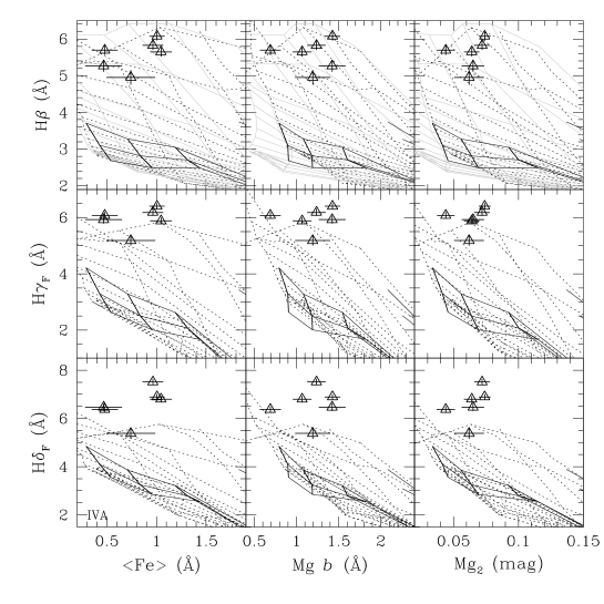
In Figure 14 we compare the Balmer-line indices of the LMC clusters with the models of [Maraston & Thomas (2000)]. We do not use the W94 models here since they do not reach to sufficiently young ages. In each of the panels in Figure 14, ages become progressively younger from the bottom-left to top right, indicating that the LMC clusters possess a significant range in age. Notice that the panels in Figure 14 which include H$\beta$ as one co-ordinate are not degenerate, demonstrating the increased age-sensitivity of H$\beta$ over the higher-order Balmer lines. No significant offsets are apparent between these indices.

5 The Ages and Metallicities of the LMC Clusters

5.1 The Loci of SWB-Types on the SSP Grids

Table 14: The SWB – age calibration of [Bica et al. (1992)] 1992.

SWB Type	Age (Gyr)
I	0.01 – 0.03
II	0.03 – 0.07
III	0.07 – 0.20
IVA	0.20 – 0.40
IVB	0.40 – 0.80
V	0.80 – 2.00
VI	2.00 – 5.00
VII	5.00 – 16.00

In principle, the position of any star cluster in the age-metallicity plane of the SSP grids indicates the age and metallicity of that stellar population. As discussed in $\S$ 2.1, SWB80 grouped the LMC clusters into SWB-types, depending upon their Q(ugr)-Q(vgr) colours. Since the SWB ranking is effectively one of age, this should be reflected in the locus of the SWB types on the SSP grids. For the convenience of the reader, we reproduce the age groups for SWB types I–VII in Table 14, as given by the calibration of [Bica et al. (1992)] (1992).

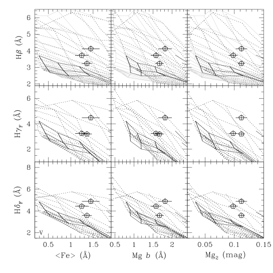
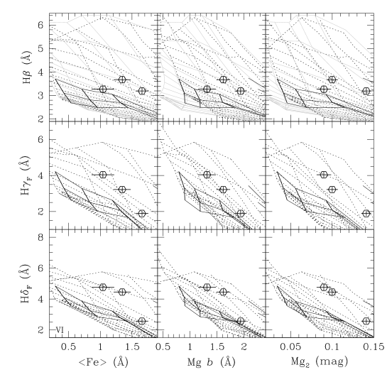
In Figures 16 to 24, we show the metallicity-sensitive $\langle$Fe$\rangle$, Mg $b$ and Mg₂ indices versus the more age-sensitive H$\beta$, H$\gamma_{F}$, and H$\delta_{F}$ indices of the LMC clusters. In each case, we compare them to the SSP models of KFF99, [Maraston & Thomas (2000)] and W94.

Our goal is to empirically test the age and metallicity predictions of SSP models which predict line-strength indices in the Lick/IDS system, rather than provide an exhaustive comparison between different models (e.g. see [Maraston et al. (2001)] 2001). However, there are clearly significant differences between the SSP models, which warrant some discussion before using them to derive ages and metallicities for the clusters.

Perhaps the most noticeable difference between the models is the much smaller parameter space covered by the W94 models As discussed in $\S$ 4.3, the majority of the LMC clusters do not fall onto the W94 grids, indicating that the W94 models will only be useful for the oldest clusters. Direct comparison between the KFF99 and [Maraston & Thomas (2000)] models shows that, in general, the KFF99 models tend to predict younger ages and higher metallicities for any given position on the grids. Also, the Mg b and Mg₂ indices predicted by the KFF99 models extend to lower values than those of [Maraston & Thomas (2000)], despite the fact that both models extend to [Fe/H] $\sim$ –2.3.

One feature of the [Maraston & Thomas (2000)] models is that, at low metallicities, the youngest isochrones turn sharply downwards, crossing over older isochrones. This is a result of Balmer line-strengths decreasing as turn-off temperatures exceed T${}_{\rm eff}\sim$ 9,500 K, at younger ages than where Balmer lines are at a maximum. The loci of the Balmer-line maximum shifts to older ages as metallicity decreases (e.g. [Maraston et al. (2001)] 2001).

An important, but subtle difference between the evolutionary synthesis models of [Maraston & Thomas (2000)] and KFF99, and the population synthesis models of W94, is the treatment of RGB stars. In the [Maraston & Thomas (2000)] and KFF99 models, mass-loss on the RGB is dealt with by using an analytical recipe (in the case of these two SSP models, Reimers’ mass-loss equation [Reimers (1975)] is adopted). The amount of mass-loss suffered by RGB stars plays a crucial r$\hat{\rm o}$le in determining the position at which these stars fall onto the HB (e.g. [Buzzoni (1989)] 1989). Lower mass RGB stars lead to bluer (hotter) HBs, and increasing the ’mass-loss parameter’ ($\eta$), pronounces this effect. As pointed out by [Rabin (1982)] (1982), the presence of such stars can potentially severely effect integrated indices, and in particular the Balmer lines.

The effect of this mass-loss can be seen in the [Maraston & Thomas (2000)] models, and to a lesser extent, those of KFF99. At old ages ($\sim$ 12 Gyr), and low metallicities ([Fe/H] $\leq$ –1.0), Balmer line-strengths begin to $increase$, rather than decrease as expect with age, creating a saddle-point minima at $\sim$ 12 Gyr. Therefore, at old ages and low metallicities, a unique solution for the age of a stellar population is not necessarily attainable with integrated indices. The interpretation of the SSP models in this regime is further discussed in $\S$ 5.4, as are the effects of HB stars on our integrated Balmer indices in $\S$ 5.4.1.

Returning to Figures 16 to 24, we find the agreement between the $\langle$Fe$\rangle$, Mg $b$ and Mg₂ indices is good. In general, the position of the clusters on the SSP grids using these different metallicity indicators are consistent within the uncertainties. The H$\beta$, H$\delta_{\rm F}$ and H$\gamma_{\rm F}$ indices also behave similarly, although there are some indications of systematic differences between their age predictions for the younger clusters.

The SWB types lie in relatively tight groups on the SSP model grids. As one goes to older SWB types in Figures 16 to 24, these groups trace a characteristic shape, moving from the top-left (young ages, [Fe/H]  $>$$\sim$ –1.0), to centre-right (intermediate ages, [Fe/H]  $>$$\sim$ –1.0), to bottom-left (old ages, [Fe/H] $<$ –1.0). One cluster in Figure 24 clearly stands out as being significantly younger than the other SWB VII clusters, and provides a nice illustration of the advantage of integrated spectroscopy over photometry in separating age and metallicity effects. This cluster, NGC 1865, has an SSP-derived age of $<$ 1.0 Gyr, rather than the $\sim$ 10 Gyr implied by its SWB type. [Geisler et al. (1997)] (1997) obtained an age of 0.9 Gyr for this cluster from the position of its CMD turnoff, which is consistent with our value. [Geisler et al. (1997)] (1997) attributed its SWB mis-classification to a combination of the stochastic effects of bright stars in the cluster, and its relative faintness contrasted with a dense stellar background.

Figure 16: Age-metallicity diagnostic diagrams for the SWB IVA clusters. Grey lines: Lick/IDS indices of the LMC clusters compared to the KFF99 SSP models. Near-horizontal lines are isochrones of 0.5, 1, 2, 3 … 16 Gyr (youngest ages at the top). Metallicity increases from left to right, with lines of –2.3, –1.7, –1.22 (interpolated), –0.7, –0.4, 0 and + 0.4 dex. Dotted lines: SSP models of Maraston & Thomas (2000). Isochrones range from 0.5, 1, 2, 3 … 15 Gyr, metallicity isopleths are –2.25, –1.35, –0.84 (interpolated), –0.33, 0 and + 0.35 dex. Solid lines: Worthey (1994) models with ages 8, 12 and 17 Gyr, and metallicities (shown) –2.0, -1.5 and –1.0.

Figure 18: Age-metallicity diagnostic diagrams for the SWB IVB clusters.

Figure 20: Age-metallicity diagnostic diagrams for the SWB V clusters.

Figure 22: Age-metallicity diagnostic diagrams for the SWB VI clusters.

Figure 24: Age-metallicity diagnostic diagrams for the SWB VII clusters.

5.2 Measuring Metallicities and Ages

As our principle metallicity indicators we have chosen our best-measured magnesium dominant Lick index (Mg₂), and mean of two iron indices (Fe5270 and Fe5335) in the form of $\langle$Fe$\rangle$. As age-sensitive indices, we use H$\beta$ ([Maraston & Thomas (2000)] and KFF99 models), in addition to our best-measured higher-order Balmer lines H$\gamma_{\rm F}$ and H$\delta_{\rm F}$ ([Maraston & Thomas (2000)] models only).

Ages and metallicities are obtained for each cluster by interpolating the model grids using a fortran programme. Where clusters lie off the grids, linear extrapolation is used. Uncertainties are derived by perturbing the line-strength indices by their corresponding measurement error. Because of the non-orthogonal nature of the model grids, two differing uncertainties in age and two differing uncertainties in metallicity are obtained. As discussed previously, due to the effects of the HB on the Balmer indices, the metal-poor, old regions models often have two age solutions for the SWB VII clusters. In these cases, we adopt the prior that these clusters are Galactic GC analogues, and adopt the older ages if the clusters are consistent with these old isochrones (see $\S$ 5.4 for futher explanation.)

Whilst we wish to compare the SSP model predictions to independently derived ages and metallicities, an important feature of the SSP models should be emphasised. Due to the non-orthogonality of the SSP grids, changes in the metallicity estimates of the clusters effect the derived ages of the clusters and vice versa – i.e.  there is still an age-metallicity degeneracy. As a direct result of this, the KFF99 models, which have a tendency to systematically over-predict metallicities with respect to the [Maraston & Thomas (2000)] models (see $\S$ 5.1), systematically under-predict the cluster ages with respect to the [Maraston & Thomas (2000)] models.

This is illustrated in Figure 26, where we compare the age and metallicity predictions of the [Maraston & Thomas (2000)] and KFF99 models using two different metallicity indicators ($\langle$Fe$\rangle$, Mg₂) and the more age-sensitive H$\beta$. The effect can be most clearly seen in the $\langle$Fe$\rangle$–H$\beta$ plane of the models. The KFF99-derived metallicities are systematically 0.2–0.5 dex higher than the [Maraston & Thomas (2000)]-derived metallicities. This leads to cluster ages which are significantly younger in the KFF99 models (up to 6 Gyr for old ages) than those of [Maraston & Thomas (2000)]. However, surprisingly, the agreement between models for the ages of the youngest clusters is much better, even though the agreement between their metallicities is poorest. The origin of these differences are unclear, since both the models use the same fitting-functions, but a possible explanation may lie in their adoption of different input isochrones.

Of final, important note in Figure 26, there is a clear offset in metallicity between the $\langle$Fe$\rangle$- and Mg₂-derived metallicities, in the sense that the Mg₂ index predicts metallicities 0.1 $\sim$ 0.5 dex higher than $\langle$Fe$\rangle$. However, we find no evidence of a significant systematic offset between our measured magnesium and iron indices. As we showed in Section 4, we were able to correct both these indices onto the Lick/IDS system.

An alternative explanation is that the $\langle$Fe$\rangle$ and Mg₂ indices do not track metallicity in the same manner; the [Fe/H] measurements of the clusters are systematically lower than our [Mg/H] measurements. Such ”$\alpha$-enhancement” has been seen in the integrated spectra of elliptical galaxies (e.g. [Peletier (1989)] 1989; Gonz$\acute{a}$lez 1993; [Kuntschner et al. (2001)] 2001; [Trager et al. (2000a)] 2000a) and recently in extragalactic globular clusters (e.g. [Forbes et al. (2001)] 2001, [Larsen et al. (2002)] 2002). Moreover, high-resolution spectroscopy of LMC clusters giants suggests that, from [O/H] ratios, this is also the case for LMC clusters [Hill et al. (2000)]. However, such an interpretation is complicated by the fact that, at low metallicities, the differences between solar-scaled and $\alpha$-enhanced SSP models are small (i.e. little dynamic range, e.g. [Milone et al. (2000)] 2000). A detailed analysis of this important issue is beyond the scope of this paper, and we defer further discussion to future work.

In Table B1, we list the age and metallicity predictions of the [Maraston & Thomas (2000)] SSP models, using the Mg₂-H$\beta$ and $\langle$Fe$\rangle$-H$\gamma_{\rm F}$ indices. To test these model predictions, we have collected age and metallicity estimates for the LMC clusters in our sample from the literature. These are also presented in Table B1. These literature ages and metallicities come from a variety sources and are therefore rather inhomogenous. Where possible, we have tried to minimise this inhomogeneity whilst retaining a large enough sample for meaningful comparisons. Cluster ages are preferentially taken from studies which have located the main sequence turn-off in CMDs. These have been supplemented with ages obtained by the giant-branch calibration of [Mould & Aaronson (1982)] (1982). For the seven clusters with no previous spectroscopic- and/or CMD-derived age determinations, we have adopted a mean age which corresponds to their SWB type (see Table 14). We assign uncertainties by taking the 50 percentiles in their SWB age-range.

Figure 26: Comparison between the age and metallicity predictions of the Maraston & Thomas and KFF99 SSP models for the $\langle$Fe$\rangle$, Mg₂ and H$\beta$ Lick/IDS indices. Solid line represents unit slope.

The majority of the literature cluster metallicities come from the $\sim$ 2 Å resolution Ca-triplet spectroscopy of cluster red giants by [Olszewski et al. (1991)] (1991). For clusters not in the [Olszewski et al. (1991)] (1991) sample, we adopt metallicities from integrated spectroscopy ([Rabin (1982)] 1982; [Dutra et al. (1999)] 1999). Ages and metallicities for NGC 1806 are from the Strömgren photometry of [Dirsch et al. (2000)] (2000).

The LMC globular clusters NGC 1754, NGC 1835, NGC 1898, NGC 2005 and NGC 2019 have metallicities from two sources. [Olsen et al. (1998)] (1998) derived metallicities for these clusters from HST CMDs by measuring the height of the HB above the main sequence turn-off (the $V^{TO}_{HB}$ method of [Sarajedini (1994)] 1994). These clusters are also included in the [Olszewski et al. (1991)] (1991) sample, and therefore have spectroscopic abundances. In the mean, the metallicities derived by [Olszewski et al. (1991)] (1991) are $\sim$ 0.3 dex lower than those found by [Olsen et al. (1998)] (1998) using the $V^{TO}_{HB}$ method. To increase the homogeneity in our metallicity comparisons, and because we prefer spectroscopic metallicities, we adopt the values of [Olszewski et al. (1991)] (1991), and the ages derived by [Olsen et al. (1998)] (1998) using these metallicities. NGC 1916 was also in the [Olsen et al. (1998)] (1998) sample, however differential reddening precluded an age determination for this cluster.

5.3 Metallicity Comparisons

We compare the metallicities of the LMC clusters derived from the various combinations of metallicity-sensitive and age-sensitive indices (using the [Maraston & Thomas (2000)] and KFF99 models) with their literature values in Figure 28. To first order, the agreement between the literature values and the metallicities from the $\langle$Fe$\rangle$ and Mg₂ indicators is satisfactory. Our mean metallicity uncertainty is $\sim$ 0.20 dex for Mg₂–H$\beta$ and $\sim$ 0.25 dex for $\langle$Fe$\rangle$–H$\beta$, generally consistent with the scatter seen in Figure 28. For the higher-order Balmer lines, the mean uncertainty increases to $\sim$ 0.3 dex due to the larger degree of age-metallicity degeneracy in the models for these indices.

There is broad agreement between different index-index combinations, as there is reasonable consistency between the [Maraston & Thomas (2000)] and KFF99 model metallicity predictions (for H$\beta$). The well documented metallicity-gap (and the corresponding age gap) of the LMC clusters is evident at [Fe/H] $\sim$ –1.0 (e.g. [Westerlund (1997)] 1997).

Figure 28: Comparison between literature metallicities of the LMC clusters, and those derived from the SSP models of Maraston & Thomas and KFF99 for different spectroscopic indices. Solid triangles represent the spectroscopic values of Olszewski et al. (1991), squares : integrated spectroscopy, pentagons : Strömgren photometry. The solid line indicates unit slope, dashed line indicates the non-linear relation between the Zinn & West (1984) and Zinn (1985) metallicity scale, and that obtained by Carretta & Gratton (1997).

Figure 30: Comparison between literature ages of the LMC clusters, and those derived from the SSP models of Maraston & Thomas and KFF99. Solid squares indicate literature ages from ground-based CMDs, pentagons : Strömgren photometry, circles : HST CMDs, open pentagons : ages from SWB types. The solid line represents unit slope.

However, closer inspection of Figure 28 reveals some interesting differences between the SSP-derived and literature metallicities. The most obvious difference is that again, the Mg₂ index predicts higher metallicities than $\langle$Fe$\rangle$. As discussed in the previous Section, in the absence of any obvious systematic errors in our data, a possible explanation is the detection of $\alpha$-enhancement in the LMC clusters.

Another discrepancy is that the low-metallicity clusters generally exhibit a systematic deviation from unit slope. Rather than showing a straight offset from the literature values, these clusters metallicities are actually better fit with a non-linear function. This behaviour is also seen to greater or lesser extents in all the other indices and in the both the KFF99 and [Maraston & Thomas (2000)] models.

Can the origin of these differences lie in the different metallicity scales of the literature LMC clusters, and the SSP models? The source of the majority of our literature cluster metallicities come from the study of [Olszewski et al. (1991)] (1991). [Olszewski et al. (1991)] (1991) calibrated their Ca-triplet measurements with Galactic GCs using metallicities on the [Zinn & West (1984)] (1984) and [Zinn (1985)] (1985; hereafter the ZW scale) scale. However, [Carretta & Gratton (1997)] (1997) have shown that, whilst the ZW scale is reassuringly monotonic, it is non-linear with respect to the solar (meteoritic) scale upon which the SSP model input isochrones are based. In the range –1.9 $\leq$ [Fe/H] $\leq$ –1.0, the ZW scale predicts metallicities $\sim$ 0.2 dex lower than the meteoritic values. For metallicities outside this range, the ZW scale yields values systematically higher than the meteoritic scale.

The relation between these two scales is illustrated in Figure 28 by the dashed line. The $x$-axis may be regarded as the ZW scale (largely [Olszewski et al. (1991)] metallicities), the $y$-axis that of [Carretta & Gratton (1997)] (1997) (the SSP models). We find that, for the $\langle$Fe$\rangle$ metallicity indicator, better agreement is generally reached using the [Carretta & Gratton (1997)] (1997) scale, including the flattening in their relation at [Fe/H] $\sim$ –0.5. This is perhaps not surprising since [Carretta & Gratton (1997)] (1997) derived metallicities from resolved Fe I lines, whilst $\langle$Fe$\rangle$ essentially measures features (iron and others) in the same wavelength range but at significantly lower resolution. However, the metallicities derived using Mg₂ are not so well reconciled, particularly with regard to the highest-metallicity clusters which actually follow a one to one correlation (unit slope) somewhat more closely. The question of which metallicity scale is to be preferred is still an open one (e.g. see [Caputo & Cassisi (2002)] 2002).

To summarise, we find good agreement between the SSP model and literature determinations for the metallicities of the LMC clusters in the range –2.0 $\leq$ [Fe/H] $\leq$ 0. Systematic offsets between the metallicities predicted by $\langle$Fe$\rangle$ and Mg₂ are possibly due to non-solar abundance ratios in the LMC clusters. Differences in the metallicity scales (from the line-blanketing indices of ZW, and Fe I scale of [Carretta & Gratton (1997)] 1997) are at most a second-order effect.

Of the 24 LMC clusters in our sample, 11 have no previous metallicity determinations. The weighted mean of the two values given in Table B1 should yield a good mean metallicity for these clusters.

5.4 Age Comparisons

Comparisons between the ages of the clusters derived from the SSP models, and those collected from the literature are presented in Figure 30. The presence of clear correlations in the figure are reassuring. Each of the Balmer indices shown in Figure 30 are, to first order at least, tracking the temperature of the main sequence turn-off in the clusters, and thereby providing a measure of cluster age.

We find that the best agreement is obtained for the intermediate-aged clusters (i.e. 1 $\sim$ 4 Gyr). The H$\beta$ index yields ages which are in excellent agreement with their CMD values, for both the iron and magnesium metallicity indicators. H$\gamma_{\rm F}$ and H$\delta_{\rm F}$ also predict ages which are generally consistent with the literature, although with somewhat larger scatter.

In the metallicity–H$\beta$ planes of both models, the youngest clusters ($<$ 1 Gyr) are predicted to be older (by 0.2 – 1.0 Gyr) than the literature ages. These H$\beta$ ages are also older than is predicted by the higher-order Balmer lines. Whilst this is only a 1–2$\sigma$ effect for any individual cluster, it is systematic. In the absence of systematic errors in the literature ages of these clusters (in the sense that the literature ages are too young), the source of this disagreement is either (i) emission fill-in of the clusters’ H$\beta$ lines or (ii) an uncertainty in the SSP models at young ages. Since we detect no emission in these clusters’ sky spectra, we conclude that, if present, any emission must be arising from some internal source. This would be plausible if these clusters were very young (i.e. $<$ 10⁷ yr) and massive O/B stars were present. However, this is not only inconsistent with their integrated colours, but also the spectra of these clusters do not show the characteristic blue continua of very young objects.

There is some evidence that the SSP models at these young ages may be at fault (for H$\beta$). The disagreement in the cluster ages occurs at $<$ 3 Gyr, coincident with were the SSP models are most uncertain due to the necessary extrapolation required in the Lick/IDS fitting-functions. Moreover, the young, metal-poor regions of the SSP grids are precisely the areas of parameter space which are inadequately covered by the spectral libraries input into the models. Clearly, this issue needs to be investigated futher with a larger sample of integrated spectra for Magellanic Cloud clusters in this age range.

We now turn to the SSP age predictions of the LMC globular clusters (SWB VII) in our sample. At this stage, the method by which we interpret the ages of the ’old’ clusters using the SSP model grids should be discussed.

In Figure 32 we show the SWB VII clusters (excluding NGC 1865 which we earlier showed to be $\sim$ 1.0 Gyr old) in the Mg₂–Balmer line planes of the [Maraston & Thomas (2000)] models. It can be seen immediately from Figure 32 that the isochrones of the oldest ages overlap with those of younger isochrones at low metallicities. Whilst this is only a weak effect in the models for H$\beta$, for H$\gamma_{\rm F}$ and H$\delta_{\rm F}$ the effect is significant. The oldest (15 Gyr) isochrone of the [Maraston & Thomas (2000)] models predicts higher-order Balmer line-strengths very similar to those of the 5 Gyr isochrone.

Figure 32: The LICK/IDS indices of the LMC globular clusters compared to the SSP models of Maraston & Thomas (2000). Symbols indicate the different clusters, filled triangle : NGC 1754, filled square : NGC 1786, filled pentagon : NGC 1835, filled hexagon : NGC 1898, open triangle : NGC 1916, open square : NGC 1939, open pentagon : NGC 2005, open hexagon : NGC 2019. Dotted grey lines indicate isochrones of 5–9 Gyr, solid grey lines are isochrones of 10–14 Gyr. The solid black line indicates the position of the oldest (15 Gyr) isochrone of the models. Dashed line indicates an interpolated line of constant metallicity at [Fe/H]=–1.22.

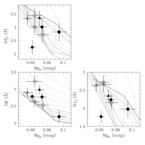
Our prior is such that the SWB VII clusters shown in Figure 32 are the LMC counterparts of Galactic GCs, and as such have ages in excess of 10 Gyr. Therefore, in interpreting the figure, the older isochrones ($>$ 10 Gyr) are adopted. These are the cluster ages listed in Table B1, and shown in Figure 30. Any clusters which lie above the oldest (15 Gyr) isochrone of the models are assigned an extrapolated age (i.e. $>$ 15 Gyr) only if their line-strengths are consistent (1$\sigma$ uncertainty) with this oldest isochrone (solid line in Figure 32). Otherwise, SWB VII clusters with strong Balmer-absorption are given younger ’spectroscopic’ ages.

The age predictions of the SSP models for the LMC globular clusters (Figure 30) show significant variations, depending upon the combination of Lick/IDS indices used. In contrast, the literature ages of the clusters (5 from the HST CMDs of [Olsen et al. (1998)] (1998), 1 from the ground-based CMD of [Geisler et al. (1997)] (1997) and 2 inferred from their SWB type) show a reasonably tight age-range, from 10 to 17 Gyr. These ages are in reasonable agreement with the ’best’ value for the Milky Way GCs of 12.9 $\pm$ 2.9 Gyr [Carretta et al. (2000)].

We find that the higher-order Balmer lines, H$\gamma_{\rm F}$ and H$\delta_{\rm F}$, are generally consistent with the CMD turn-off ages and/or integrated colours. However, H$\beta$, the most age-sensitive of the Lick/IDS indices [Worthey & Ottaviani (1997)] predicts a couple of clusters to be significantly younger than is indicated by their literature values. Specifically, the two clusters, NGC 1754 and NGC 2005, have SSP model ages which are inconsistent with the literature at 3$\sigma$ significance. Both of these clusters have well-developed blue HBs, and their influence upon the integrated Balmer indices we examine shortly.

As shown in Figure 32, we also find that the position of NGC 1786 stands out in the H$\gamma_{\rm F}$ and H$\delta_{\rm F}$ planes of the SSP models. However, these indices of this cluster only fall below the [Maraston & Thomas (2000)] model isochrones at the $\sim$ 2$\sigma$ level, and therefore we do not ascribe them any particular significance.

5.4.1 The Effect of Horizontal Branch Stars on Integrated Balmer Indices

In the previous section, we found two GCs, NGC 1754 and NGC 2005, have SSP-derived ages significantly (3$\sigma$) younger than the literature values. [Rabin (1982)] (1982) was the first to suggest that the presence of blue HB stars may have a significant effect upon the equivalent width of the Balmer indices, possibly comparable to the contribution from stars at the main sequence turn-off. Since NGC 2005 has a largely blue HB, is it possible that the presence of blue HB stars are the origin of this present disagreement with the SSP models? Looking at this issue, [de Freitas Pacheco & Barbuy (1995)] (1995) compared the H$\beta$ line-strengths of 10 Galactic GCs with their HB morphologies. With the aid of empirical modelling, these authors suggested that Blue HBs may increase H$\beta$ by upwards of $\sim$ 1.0 Å.

For the five clusters in our sample with HST CMDs from [Olsen et al. (1998)] (1998), we have an accurate measure of their CMD age, HB morphology and integrated Balmer indices. Since these clusters (NGC 1754, NGC 1835, NGC 1898, NGC 2005 and NGC 2019) all have similar mean spectroscopic metallicities (mean metallicities derived from Table B1 are [Fe/H] = –1.38, –1.57, –1.30, –1.43 and –1.42 respectively), we are able to directly compare the effect of HB morphology upon the Lick/IDS Balmer indices of the LMC clusters.

Figure 34: Balmer line-strength plotted against the HB parameter $(B-R)/(B+V+R)$ of five LMC globular clusters. Filled triangle : NGC 1754, filled pentagon : NGC 1835, filled hexagon : NGC 1898, open pentagon : NGC 2005 and open hexagon : NGC 2019.

We plot the Lick/IDS Balmer indices of these GCs against their respective HB parameters in Figure 34. The HB parameter (e.g. [Lee et al. (1994)] 1994) is commonly given by $(B-R)/(B+V+R)$, where $B$ is the number of HB stars to the blue of the instability strip, $V$ the number of RR Lyrae stars and $R$ the number of HB stars redward of the instability strip. Negative values of this parameter indicate a red HB morphology (–1 corresponds to no blue HB stars), increasingly positive numbers correspond to progressively bluer HBs.

As shown in Figure 34, there is a correlation between HB parameter and Balmer line-strength, in the sense that bluer HBs lead to larger index values for H$\beta$, H$\gamma_{\rm F}$ and H$\delta_{\rm F}$. NGC 1898, which has a roughly equal number of stars to the left and right of its RR Lyrae variables (and has the reddest determined HB morphology in our sample), has H$\beta$ line-strengths $\sim$ 1 Å lower than that of NGC 2005, a cluster which has a blue HB.

If we temporarily ignore the possible contribution from HB stars, at a given metallicity, a change in $\sim$ 1 Å in H$\beta$ would be interpreted as an age difference of $>$ 10 Gyr using the (extrapolated) W94 models. Since [Olsen et al. (1998)] (1998) obtained a CMD age for NGC 1898 of 14.0 $\pm$ 2.3 Gyr, and for NGC 2005 of 16.6 $\pm$ 5.1 Gyr (assuming [Olszewski et al. (1991)] 1991 abundances), the possibility of a 10 Gyr age difference between these two clusters seems unlikely.

One possible origin of this behaviour of the Balmer lines is the metallicity dependence of the integrated indices themselves. We found in this study that the metallicities of the clusters in Figure 34 are very similar. This is also true of the metallicities derived by [Olsen et al. (1998)] (1998) for these same clusters, using the $V^{TO}_{HB}$ method of [Sarajedini (1994)] (1994). However, [Olszewski et al. (1991)] (1991) found from their Ca-Triplet observations that NGC 2005 was some $\sim$ –0.5 dex more metal-poor than NGC 1898. Since the Lick/IDS H$\beta$ index is really a blend of many metallic lines, centred on the H$\beta$ feature, significant metallicity differences amongst the clusters may be driving variations in this index.

To test this possibility, we have used the W94 SSP models which do not account for variations in HB morphology, but treat HB stars purely as a red clump. The predictions of these models are qualitatively very similar to SSP models with no HB stars (e.g. W94; [Lee et al. (2000)] 2000). The W94 models predict that H$\beta$ increases very slowly with decreasing metallicity at old ages. At 17 Gyr, they indicate that H$\beta$ increases by +0.12 Å from [Fe/H] = –1.5 to [Fe/H] = –2.0. Moreover, this increase in H$\beta$ becomes only slightly larger for younger ages, +0.17 Å at 12 Gyr and + 0.27 Å at 8 Gyr. Therefore, even if NGC 2005 is –0.5 dex more metal-poor than NGC 1898, the metallicity sensitivity of Balmer lines themselves cannot explain the position of the GCs in Figure 34.

We conclude that the Balmer-line indices of the LMC GCs are significantly effected (increased by up to $\sim$ 1.0 Å in H$\beta$) by the presence of blue HB stars. The [Maraston & Thomas (2000)] (2000) and KFF99 models try to account for this dependency of HB morphology on metallicity, and its subsequent contribution to the Balmer lines, by including mass-loss of the RGB. However, a shift of –0.5 dex in the [Maraston & Thomas (2000)] models corresponds to an increase in H$\beta$ of only $\sim$ 0.5 Å at old ages and low metallicities, inconsistent with the ages of NGC 1754 and NGC 2005.

This, however, is no real fault of the models; HB morphology cannot not be directly predicted from first principles in stellar evolution. The unknown mechanisms for mass-loss must be subsumed within an analytical expression such as Reimer’s formalism (among others) which has little physical basis. Moreover, the HB morphologies of GCs are not a monotonic function of metallicity, and require at least one more parameter to describe their morphology. This “second parameter effect” is thought to be age, although the issue is far from settled (e.g. [Lee et al. (1994)] 1994). Therefore, since SSP models cannot directly predict HB morphologies, they must be calibrated from observations of real GCs (e.g. [Lee et al. (2000)] 2000).

Finally, we note that in the HST CMD for NGC 1898 from [Olsen et al. (1998)] (1998), there are a number of stars which lie in the location on the CMD consistent with blue straggler stars (i.e. $V-I$ $\sim$ 0.2, $V\sim$ 21). Whilst [Olsen et al. (1998)] (1998) make no such claim, due to uncertainties in their CMD-cleaning procedure, the possibility that they are blue stragglers is intriguing. The location of this cluster on the SSP grids suggests that if these are indeed blue straggler stars, they do not contribute significantly the Balmer indices of NGC 1898 (e.g. see [Burstein et al. (1984)] 1984 and [Trager et al. (2000b)] 2000b).

A more detailed comparative study of the blue straggler population, and their effects on integrated indices, should be performed between Galactic (or otherwise) GCs with very similar metallicities, ages and HB morphologies.

6 Summary and Conclusions

We have obtained high S/N integrated spectra for 24 star clusters in the LMC, and derived age and metallicity estimates for these clusters using a combination of the Lick/IDS indices and the SSP models of [Maraston & Thomas (2000)] (2000) and [Kurth et al. (1999)] (1999). To test the SSP models, we have compiled a list of metallicity and age determinations from the literature. Metallicities were taken largely from the Ca-Triplet spectroscopy of [Olszewski et al. (1991)] (1991). The age estimates are somewhat more inhomogeneous in nature, deriving from a number of methods; the location of the main-sequence turn-off in CMDs, the extent of the AGB calibration of [Mould & Aaronson (1982)] (1982) or integrated colours. Comparing these independently derived quantities we find:

• the SSP-derived metallicities, obtained using both the Mg₂ and $\langle$Fe$\rangle$ Lick/IDS indices show generally good agreement with the literature values. However, the Mg₂ index (and to a lesser degree Mg $b$) predicts metallicities which are systematically higher than those from $\langle$Fe$\rangle$, by up to +0.5 dex for the highest metallicity clusters. Amongst the possible explanations for this difference is the existence of [$\alpha$/Fe] $>$ 0 in the clusters. We publish metallicities for 11 LMC star clusters with no previous measurements, which are accurate to $\sim$ 0.2 dex.

• for the majority of the LMC clusters, the SSP-models predict ages from the H$\beta$, H$\gamma_{\rm F}$ and H$\delta_{\rm F}$ indices which are consistent with the literature values. However, age estimates of the old LMC globular clusters are often ambiguous. The oldest isochrones of the SSP models overlap younger isochrones due to the modelling of mass-loss on the RGB. Assuming old ages in interpreting these data, six clusters, NGC 1786, NGC 1835, NGC 1898, NGC 1916, NGC 1939 and NGC 2019, have SSP-derived ages in all three measurable Balmer indices which are consistent with their ages derived from CMDS or integrated colours.

• two clusters, namely NGC 1754 and NGC 2005, have extremely strong Balmer lines, which leads to the SSP model ages which are too young ($\sim$ 8 and 6 Gyr respectively). Comparison between the horizontal branch morphology and the Balmer lines for five of the GCs in our sample suggests that blue HBs are likely contributing up to $\sim$ 1.0 Å to the H$\beta$ index in these clusters.

We conclude that the SSP models considered in this study are able to satisfactorily predict the ages and metallicities for the vast majority of LMC star clusters from integrated spectroscopic indices. This remains true despite the rather inhomogenous nature of the literature age determinations. However, estimating the ages of the old, low-metallicity LMC GCs is severely complicated by the strong contribution of horizontal branch/post-horizontal branch stars to integrated indices. We conclude that at old ages and low metallicities ([Fe/H] $<$ –1.0), Balmer lines (e.g. H$\beta$, H$\gamma$, H$\delta$) are not useful age indicators without a priori knowledge of horizontal branch morphology.

7 Acknowledgements

We wish to thank Hyun-chul Lee for useful comments regarding this paper, Mike Reid for the preparation of UKST finding charts, and Malcolm Hartley, who went above and beyond the call of duty during the FLAIR observations. We are in debt to Claudia Maraston for interesting discussions and for providing her full models ahead of publication, and the anonymous referee for their detailed appraisal of the paper. MB acknowledges the Royal Society for its fellowship grant.

A Corrected Lick Indices for LMC Star Clusters

The Lick/IDS indices for 24 LMC star clusters after the additive corrections are applied (Table 12) are given in Table A1. The uncertainties are tabulated in alternate rows, calculated from the S/N of the spectra added in quadrature to our index repeatability which is given in Table 10.

Table A2: Lick/IDS indices for LMC star clusters. Uncertainties tabulated in alternate rows are calculated from the S/N of the spectra added in quadrature to our repeatability of each index.

ID	CN1	CN2	Ca4227	G4300	Fe4383	Ca4455	Fe4531	C4668	H$\beta$	Fe5015
	(mag)	(mag)	(Å)	(Å)	(Å)	(Å)	(Å)	(Å)	(Å)	(Å)
NGC 1718	–0.141	–0.087	0.267	1.747	0.549	0.167	0.966	–0.183	3.265	2.444
$\pm$	0.018	0.021	0.153	0.310	0.366	0.196	0.966	0.413	0.169	0.428
NGC 1751	–0.142	–0.112	1.158	2.360	1.978	0.255	1.565	2.083	4.122	4.396
$\pm$	0.019	0.023	0.158	0.330	0.401	0.219	1.565	0.451	0.177	0.449
NGC 1754	–0.122	–0.082	0.830	1.707	0.909	0.156	1.349	–0.218	2.981	2.755
$\pm$	0.011	0.013	0.100	0.238	0.235	0.135	1.349	0.286	0.127	0.349
NGC 1786	–0.084	–0.040	0.468	1.771	0.743	0.450	1.273	–0.666	2.210	1.662
$\pm$	0.006	0.008	0.075	0.205	0.164	0.106	1.273	0.219	0.110	0.317
NGC 1801	–0.188	–0.127	0.237	–2.320	–0.607	0.281	0.675	–0.662	5.694	1.737
$\pm$	0.009	0.012	0.092	0.235	0.226	0.132	0.675	0.290	0.129	0.362
NGC 1806	–0.099	–0.041	0.432	1.184	0.642	0.866	2.175	0.784	3.230	3.616
$\pm$	0.011	0.013	0.103	0.241	0.240	0.137	2.175	0.288	0.131	0.354
NGC 1830	–0.207	–0.141	0.600	–1.911	–1.093	–0.503	1.692	0.319	4.953	2.051
$\pm$	0.020	0.025	0.173	0.374	0.451	0.238	1.692	0.507	0.197	0.506
NGC 1835	–0.106	–0.054	0.403	1.662	0.832	0.426	1.320	–0.237	2.771	2.531
$\pm$	0.010	0.013	0.098	0.233	0.225	0.132	1.320	0.274	0.125	0.343
NGC 1846	–0.176	–0.118	0.880	0.882	0.856	0.470	2.498	–0.265	3.672	2.752
$\pm$	0.014	0.016	0.120	0.269	0.283	0.156	2.498	0.326	0.139	0.373
NGC 1852	–0.122	–0.069	0.769	1.033	0.290	0.273	1.786	0.201	3.723	3.436
$\pm$	0.013	0.015	0.117	0.265	0.288	0.160	1.786	0.340	0.146	0.385
NGC 1856	–0.205	–0.129	0.538	–1.447	0.389	0.334	1.222	0.040	6.076	2.568
$\pm$	0.007	0.009	0.077	0.212	0.175	0.111	1.222	0.232	0.112	0.325
NGC 1865	–0.224	–0.174	0.566	–0.473	0.164	0.301	1.295	–0.646	5.506	1.844
$\pm$	0.015	0.018	0.133	0.297	0.343	0.186	1.295	0.409	0.164	0.441
NGC 1872	–0.201	–0.139	0.255	–1.685	–0.042	0.492	0.919	–0.609	5.269	0.745
$\pm$	0.014	0.016	0.124	0.285	0.311	0.170	0.919	0.379	0.155	0.422
NGC 1878	–0.218	–0.141	0.481	–1.021	–0.682	0.237	2.061	–0.427	5.824	2.371
$\pm$	0.010	0.012	0.093	0.234	0.221	0.129	2.061	0.273	0.122	0.346
NGC 1898	–0.074	–0.017	0.646	2.634	1.044	1.452	1.910	0.583	2.191	2.195
$\pm$	0.021	0.025	0.178	0.346	0.439	0.223	1.910	0.479	0.190	0.463
NGC 1916	–0.117	–0.079	0.196	0.889	0.882	0.334	1.560	–0.001	2.840	2.075
$\pm$	0.011	0.013	0.102	0.240	0.239	0.138	1.560	0.293	0.132	0.355
NGC 1939	–0.102	–0.051	0.553	0.729	–0.168	0.268	0.325	–0.605	2.628	2.056
$\pm$	0.013	0.015	0.117	0.260	0.285	0.159	0.325	0.340	0.144	0.384
NGC 1978	–0.106	–0.070	0.820	2.746	1.766	0.702	2.465	2.597	3.188	3.986
$\pm$	0.012	0.014	0.106	0.243	0.242	0.138	2.465	0.280	0.127	0.346
NGC 1987	–0.204	–0.154	0.422	0.151	1.055	0.494	2.054	1.424	3.911	3.675
$\pm$	0.012	0.014	0.110	0.257	0.262	0.149	2.054	0.316	0.139	0.370
NGC 2005	–0.113	–0.047	0.533	0.934	1.513	0.669	1.327	–2.303	3.227	2.150
$\pm$	0.016	0.020	0.150	0.312	0.364	0.198	1.327	0.449	0.175	0.445
NGC 2019	–0.103	–0.049	0.762	0.892	0.527	0.328	1.960	0.253	2.531	2.005
$\pm$	0.015	0.017	0.126	0.276	0.307	0.169	1.960	0.364	0.153	0.398
NGC 2107	–0.200	–0.143	0.592	–1.340	0.003	0.475	1.503	–1.499	5.649	1.649
$\pm$	0.010	0.012	0.091	0.234	0.219	0.129	1.503	0.277	0.123	0.348
NGC 2108	–0.164	–0.120	1.190	1.239	–0.021	–0.082	2.361	0.565	3.828	2.207
$\pm$	0.018	0.021	0.144	0.312	0.361	0.192	2.361	0.392	0.160	0.411
SL 250	–0.148	–0.081	0.506	–0.465	–0.960	0.189	1.488	–0.095	4.223	3.528
$\pm$	0.012	0.014	0.106	0.253	0.266	0.148	1.488	0.316	0.139	0.374

Table A2

ID	Mg1	Mg2	Mg $b$	Fe5270	Fe5335	Fe5406	H$\delta_{\rm A}$	H$\gamma_{\rm A}$	H$\delta_{\rm F}$	H$\gamma_{\rm F}$
	(mag)	(mag)	(Å)	(Å)	(Å)	(Å)	(Å)	(Å)	(Å)	(Å)
NGC 1718	0.029	0.090	1.316	1.057	1.027	1.179	6.168	3.321	4.761	4.038
$\pm$	0.007	0.009	0.164	0.199	0.213	0.183	0.407	0.279	0.317	0.208
NGC 1751	0.036	0.112	1.815	1.634	1.261	0.697	6.288	3.245	4.880	4.478
$\pm$	0.008	0.009	0.177	0.211	0.234	0.199	0.418	0.303	0.324	0.217
NGC 1754	0.022	0.071	1.451	1.164	0.886	0.430	4.462	1.825	3.354	2.345
$\pm$	0.004	0.006	0.109	0.146	0.150	0.140	0.347	0.214	0.282	0.180
NGC 1786	0.020	0.062	1.274	0.753	0.703	0.160	3.065	1.200	2.251	2.172
$\pm$	0.002	0.004	0.085	0.123	0.118	0.120	0.320	0.185	0.266	0.167
NGC 1801	0.014	0.044	0.690	0.530	0.429	–0.335	9.074	8.370	6.372	6.076
$\pm$	0.005	0.007	0.123	0.161	0.171	0.156	0.330	0.199	0.271	0.172
NGC 1806	0.051	0.112	1.668	1.659	1.063	1.196	5.202	3.547	3.582	3.190
$\pm$	0.004	0.006	0.116	0.149	0.155	0.143	0.346	0.215	0.282	0.180
NGC 1830	–0.001	0.062	1.192	0.843	0.641	–0.035	8.152	7.026	5.380	5.183
$\pm$	0.009	0.011	0.208	0.248	0.282	0.235	0.422	0.298	0.331	0.221
NGC 1835	0.024	0.074	1.359	0.878	0.755	0.251	4.022	1.361	3.019	2.238
$\pm$	0.004	0.006	0.106	0.142	0.145	0.136	0.343	0.211	0.279	0.178
NGC 1846	0.025	0.100	1.617	1.590	1.101	0.605	6.271	3.456	4.450	3.219
$\pm$	0.005	0.007	0.128	0.165	0.173	0.156	0.372	0.237	0.298	0.190
NGC 1852	0.033	0.098	1.576	1.384	1.107	0.610	6.263	3.285	4.427	3.237
$\pm$	0.006	0.008	0.137	0.173	0.185	0.163	0.356	0.236	0.288	0.190
NGC 1856	0.022	0.074	1.428	0.870	1.141	0.579	9.626	8.066	6.894	6.403
$\pm$	0.003	0.004	0.093	0.130	0.129	0.127	0.319	0.185	0.265	0.166
NGC 1865	0.032	0.094	1.767	1.031	0.912	–0.154	10.400	7.051	6.511	5.707
$\pm$	0.008	0.009	0.171	0.213	0.234	0.201	0.363	0.250	0.292	0.195
NGC 1872	0.010	0.065	1.423	0.729	0.207	0.224	9.446	8.169	6.471	5.926
$\pm$	0.007	0.009	0.159	0.199	0.223	0.192	0.357	0.234	0.288	0.188
NGC 1878	0.019	0.072	1.237	0.737	1.191	0.625	10.980	8.177	7.518	6.183
$\pm$	0.004	0.006	0.109	0.145	0.148	0.139	0.330	0.199	0.272	0.172
NGC 1898	0.045	0.095	1.951	1.057	1.419	0.842	1.028	–0.071	2.830	1.980
$\pm$	0.008	0.009	0.176	0.212	0.228	0.194	0.459	0.333	0.341	0.236
NGC 1916	0.016	0.056	1.032	0.765	0.703	0.187	4.841	2.565	3.339	2.635
$\pm$	0.004	0.006	0.115	0.150	0.156	0.144	0.342	0.215	0.279	0.180
NGC 1939	0.012	0.065	1.560	0.638	0.694	0.593	4.220	3.119	3.017	2.723
$\pm$	0.006	0.007	0.134	0.170	0.181	0.159	0.359	0.234	0.289	0.189
NGC 1978	0.056	0.141	1.938	1.772	1.539	0.573	3.493	0.755	2.566	1.888
$\pm$	0.004	0.006	0.109	0.143	0.147	0.138	0.359	0.223	0.289	0.184
NGC 1987	0.041	0.121	1.775	1.341	0.960	0.622	8.526	5.645	5.453	4.553
$\pm$	0.005	0.007	0.127	0.164	0.175	0.156	0.347	0.222	0.283	0.183
NGC 2005	0.013	0.065	1.343	0.803	1.127	0.257	4.613	2.246	3.446	2.661
$\pm$	0.008	0.009	0.171	0.209	0.229	0.197	0.392	0.282	0.310	0.212
NGC 2019	0.012	0.075	1.201	1.175	0.730	0.686	3.305	2.257	2.725	2.157
$\pm$	0.006	0.008	0.143	0.178	0.194	0.169	0.374	0.248	0.298	0.197
NGC 2107	0.022	0.064	1.067	1.005	1.086	0.198	9.695	7.542	6.800	5.885
$\pm$	0.004	0.006	0.111	0.147	0.152	0.143	0.332	0.199	0.273	0.172
NGC 2108	0.040	0.108	1.385	1.599	1.760	0.916	7.052	6.401	4.768	4.988
$\pm$	0.007	0.009	0.151	0.184	0.193	0.171	0.411	0.266	0.323	0.204
SL 250	0.018	0.085	1.292	1.242	0.812	0.232	7.878	6.355	5.358	4.536
$\pm$	0.005	0.007	0.132	0.168	0.181	0.161	0.345	0.217	0.281	0.181

B Age and Metallicity Predictions of SSP Models

Table B1 lists the age and metallicities of the LMC clusters derived using the Maraston SSP models, from the H$\beta$–Mg₂ and H$\gamma_{\rm F}$–$\langle$Fe$\rangle$ Lick/IDS indices. Also tabulated are the available literature ages and metallicities for these clusters.

Table B2: Ages and metallicities of LMC star clusters.

ID	[Fe/H]	Age (Gyr)	[Fe/H]	Age (Gyr)	[Fe/H]	Age (Gyr)	Sources
	(Mg2,H$\beta$)	(Mg2,H$\beta$)	($\langle$Fe$\rangle$,H$\gamma_{\rm F})$	($\langle$Fe$\rangle$,H$\gamma_{\rm F}$)	(literature)	(literature)
NGC 1718	–1.12${}_{-0.22}^{+0.18}$	4.91${}_{-0.74}^{+0.53}$	–0.98${}_{-0.30}^{+0.29}$	1.98${}_{-0.53}^{+0.88}$	…	1.81$\pm$0.31	…,3
NGC 1751	–0.39${}_{-0.32}^{+0.25}$	2.31${}_{-0.72}^{+0.43}$	–0.42${}_{-0.23}^{+0.29}$	0.92${}_{-0.06}^{+0.25}$	–0.18$\pm$0.20	1.48$\pm$0.55	5,1
NGC 1754	–1.37${}_{-0.12}^{+0.21}$	7.00${}_{-2.00}^{+1.50}$	–1.38${}_{-0.14}^{+0.13}$	14.00${}_{-0.54}^{+1.00}$	–1.54$\pm$0.20(–1.42$\pm$0.15*)	15.6$\pm$2.3(15.6$\pm$2.2*)	5,8
NGC 1786	–1.58${}_{-0.12}^{+0.13}$	15.30${}_{-1.00}^{+1.40}$	–1.63${}_{-0.12}^{+0.11}$	…	–1.87$\pm$0.20	15.1$\pm$3.1	5,7
NGC 1801	–1.01${}_{-0.32}^{+0.23}$	0.47${}_{-0.04}^{+0.02}$	–0.98${}_{-0.28}^{+0.27}$	0.80${}_{-0.57}^{+0.28}$	…	0.30$\pm$0.10	…,11
NGC 1806	–0.71${}_{-0.16}^{+0.15}$	3.49${}_{-0.47}^{+0.05}$	–0.73${}_{-0.16}^{+0.17}$	1.59${}_{-0.39}^{+0.53}$	–0.71$\pm$0.74	0.50$\pm$0.10	10
NGC 1830	–1.02${}_{-0.40}^{+0.19}$	1.23${}_{-0.89}^{+0.38}$	–1.30${}_{-0.17}^{+0.51}$	1.50${}_{-0.29}^{+0.63}$	…	0.30$\pm$0.10	…,11
NGC 1835	–1.40${}_{-0.13}^{+0.18}$	8.31${}_{-1.80}^{+1.80}$	–1.74${}_{-0.16}^{+0.22}$	12.50${}_{-2.00}^{+1.50}$	–1.72$\pm$0.20(–1.62$\pm$0.15*)	16.6$\pm$2.9(16.2$\pm$2.8*)	5,8
NGC 1846	–0.80${}_{-0.14}^{+0.14}$	3.10${}_{-0.46}^{+0.07}$	–0.75${}_{-0.18}^{+0.20}$	1.69${}_{-0.61}^{+0.67}$	–0.70$\pm$0.20	2.85$\pm$1.10	5,1
NGC 1852	–0.85${}_{-0.15}^{+0.15}$	2.99${}_{-0.36}^{+0.08}$	–0.88${}_{-0.19}^{+0.20}$	2.30${}_{-0.36}^{+1.03}$	…	2.51$\pm$0.93	…,1
NGC 1856	–0.25${}_{-0.18}^{+0.19}$	0.60${}_{-0.10}^{+0.06}$	–0.09${}_{-0.10}^{+0.19}$	0.34${}_{-0.09}^{+0.02}$	…	0.12$\pm$0.03	…,4
NGC 1865	–0.41${}_{-0.12}^{+0.33}$	0.72${}_{-0.05}^{+0.07}$	–0.46${}_{-0.27}^{+0.25}$	0.63${}_{-0.21}^{+0.12}$	…	0.89$\pm$0.33	…,7
NGC 1872	–0.72${}_{-0.30}^{+0.10}$	1.02${}_{-0.21}^{+0.12}$	–0.72${}_{-0.16}^{+0.12}$	0.14${}_{-0.18}^{+0.21}$	…	0.30$\pm$0.10	…,11
NGC 1878	–0.29${}_{-0.35}^{+0.15}$	0.37${}_{-0.15}^{+0.18}$	–0.24${}_{-0.14}^{+0.14}$	0.38${}_{-0.02}^{+0.02}$	…	0.30$\pm$0.10	…,11
NGC 1898	–1.27${}_{-0.15}^{+0.20}$	11.01${}_{-1.83}^{+2.00}$	–1.32${}_{-0.15}^{+0.33}$	13.70${}_{-1.00}^{+1.30}$	–1.37$\pm$0.20(–1.18$\pm$0.16*)	14.0$\pm$2.3(13.5$\pm$2.2*)	5,8
NGC 1916	–2.10${}_{-0.19}^{+0.20}$	15.30${}_{-2.23}^{+4.00}$	–1.80${}_{-0.20}^{+0.20}$	14.54${}_{-1.50}^{+3.00}$	–2.08$\pm$0.20	10.5$\pm$5.5	5,11
NGC 1939	–1.55${}_{-0.36}^{+0.10}$	15.00${}_{-2.03}^{+3.02}$	–2.01${}_{-0.23}^{+0.36}$	15.20${}_{-2.00}^{+4.10}$	–2.00$\pm$0.20	10.5$\pm$5.5	9,11
NGC 1978	–0.21${}_{-0.26}^{+0.25}$	1.52${}_{-0.38}^{+0.32}$	–0.58${}_{-0.16}^{+0.15}$	1.34${}_{-0.94}^{+2.41}$	–0.42$\pm$0.20	2.00$\pm$0.74	5,7
NGC 1987	–0.42${}_{-0.14}^{+0.26}$	2.42${}_{-0.06}^{+0.31}$	–0.79${}_{-0.19}^{+0.21}$	0.84${}_{-0.22}^{+0.03}$	–0.50$\pm$0.20	2.51$\pm$0.93	2,1
NGC 2005	–1.51${}_{-0.31}^{+0.12}$	6.27${}_{-1.96}^{+1.22}$	–1.34${}_{-0.32}^{+0.26}$	16.00${}_{-1.50}^{+1.99}$	–1.92$\pm$0.20(–1.35$\pm$0.15*)	16.6$\pm$5.1(15.5$\pm$4.9*)	5,8
NGC 2019	–1.41${}_{-0.20}^{+0.40}$	16.00${}_{-3.04}^{+2.22}$	–1.44${}_{-0.37}^{+0.16}$	13.30${}_{-1.00}^{+0.80}$	–1.81$\pm$0.20(–1.23$\pm$0.15*)	17.8$\pm$3.2(16.3$\pm$3.1*)	5,8
NGC 2107	–0.64${}_{-0.56}^{+0.21}$	0.46${}_{-0.35}^{+0.23}$	–0.30${}_{-0.14}^{+0.13}$	0.48${}_{-0.04}^{+0.02}$	…	1.00$\pm$0.37	…,1
NGC 2108	–0.74${}_{-0.16}^{+0.35}$	3.02${}_{-0.10}^{+0.46}$	–0.22${}_{-0.22}^{+0.22}$	0.56${}_{-0.09}^{+0.03}$	…	0.59$\pm$0.22	…,6
SL 250	–1.00${}_{-0.12}^{+0.37}$	2.86${}_{-0.40}^{+0.42}$	–0.97${}_{-0.18}^{+0.21}$	1.24${}_{-0.28}^{+0.46}$	…	0.60$\pm$0.20	…,11

Sources: 1 = CMD, [Mould & Aaronson (1982)] (1982); 2 = Integrated Spectroscopy, [Rabin (1982)] (1982); 3 = CMD, [Elson & Fall (1988)] (1988); 4 = CMD, [Hodge & Lee (1984)] (1984); 5 = Spectroscopy, [Olszewski et al. (1991)] (1991); 6 = CMD, [Corsi et al. (1994)] (1994); 7 = CMD, [Geisler et al. (1997)] (1997); 8 = HST CMD, [Olsen et al. (1998)] (1998); 9 = Integrated Spectroscopy, [Dutra et al. (1999)] (1999); 10 = Strömgren photometry, [Dirsch et al. (2000)] (2000);
11 = ages inferred from the SWB type of the cluster. * metallicities obtained using the method of [Sarajedini (1994)] (1994).

References

- Beasley et al. (2000) Beasley M. A., Sharples R. M., Bridges T. J., Hanes D. A., Zepf S. E., Ashman K. M., Geisler D., 2000, MNRAS, 318, 1249
- Bica et al. (1992) Bica E., Claria J. J., Dottori H., 1992, AJ, 103, 1859
- Bica et al. (1996) Bica E., Claria J. J., Dottori H., Santos J. F. C., Piatti A. E., 1996, ApJS, 102, 57
- Bica et al. (1999) Bica E. L. D., Schmitt H. R., Dutra C. M., Oliveira H. L., 1999, AJ, 117, 238
- Borges et al. (1995) Borges A. C., Idiart T. P., de Freitas Pacheco J. A., Thevenin F., 1995, AJ, 110, 2408
- Burstein et al. (1984) Burstein D., Faber S. M., Gaskell C. M., Krumm N., 1984, ApJ, 287, 586
- Burstein et al. (1986) Burstein D., Faber S. M., Gonzalez J. J., 1986, AJ, 91, 1130
- Buzzoni (1989) Buzzoni A., 1989, ApJS, 71, 817
- Caputo & Cassisi (2002) Caputo F., Cassisi S., 2002, MNRAS, in press (astro-ph/0202501)
- Carretta & Gratton (1997) Carretta E., Gratton R. G., 1997, AAPS, 121, 95
- Carretta et al. (2000) Carretta E., Gratton R. G., Clementini G., Fusi Pecci F., 2000, ApJ, 533, 215
- Cassisi et al. (1998) Cassisi S., Castellani V., degl’Innocenti S., Weiss A., 1998, AAPS, 129, 267
- Castellani et al. (2001) Castellani V., Degl’Innocenti S., Prada Moroni P. G., 2001, MNRAS, 320, 66
- Cohen et al. (1998) Cohen J. G., Blakeslee J. P., Ryzhov A., 1998, ApJ, 496, 808
- Corsi et al. (1994) Corsi C. E., Buonanno R., Fusi Pecci F., Ferraro F. R., Testa V., Greggio L., 1994, MNRAS, 271, 385
- Davies et al. (1993) Davies R. L., Sadler E. M., Peletier R. F., 1993, MNRAS, 262, 650
- de Freitas Pacheco & Barbuy (1995) de Freitas Pacheco J. A., Barbuy B., 1995, AAP, 302, 718
- Dirsch et al. (2000) Dirsch B., Richtler T., Gieren W. P., Hilker M., 2000, AAP, 360, 133
- Dutra et al. (1999) Dutra C. M., Bica E., Claria J. J., Piatti A. E., 1999, MNRAS, 305, 373
- Elson & Fall (1988) Elson R. A., Fall S. M., 1988, AJ, 96, 1383
- Elson & Fall (1985) Elson R. A. W., Fall S. M., 1985, ApJ, 299, 211
- Faber (1972) Faber S. M., 1972, AAP, 20, 361
- Faber et al. (1985) Faber S. M., Friel E. D., Burstein D., Gaskell C. M., 1985, ApJS, 57, 711
- Fagotto et al. (1994) Fagotto F., Bressan A., Bertelli G., Chiosi C., 1994, AAPS, 105, 39
- Fisher et al. (1995) Fisher D., Franx M., Illingworth G., 1995, ApJ, 448, 119
- Forbes et al. (2001) Forbes D. A., Beasley M. A., Brodie J. P., Kissler-Patig M., 2001, ApJ Lett., 563, L143
- Frenk & Fall (1982) Frenk C. S., Fall S. M., 1982, MNRAS, 199, 565
- Fusi Pecci et al. (1996) Fusi Pecci F. et al., 1996, AJ, 112, 1461
- Geisler et al. (1997) Geisler D., Bica E., Dottori H., Claria J. J., Piatti A. E., Santos J. F. C., 1997, AJ, 114, 1920
- Gibson et al. (1999) Gibson B. K., Madgwick D. S., Jones L. A., Da Costa G. S., Norris J. E., 1999, AJ, 118, 1268
- González (1993) González J. J., 1993, Ph.D. thesis. Univ. Calif., Santa Cruz (G93), (1993)
- Gorgas et al. (1993) Gorgas J., Faber S. M., Burstein D., Gonzalez J. J., Courteau S., Prosser C., 1993, ApJS, 86, 153
- Harris et al. (1999) Harris G. L. H., Harris W. E., Poole G. B., 1999, AJ, 117, 855
- Harris et al. (1998) Harris G. L. H., Poole G. B., Harris W. E., 1998, AJ, 116, 2866
- Hill et al. (2000) Hill V., François P., Spite M., Primas F., Spite F., 2000, AAP, 364, L19
- Hodge & Lee (1984) Hodge P. W., Lee S.-O., 1984, ApJ, 276, 509
- Holland et al. (1996) Holland S., Fahlman G. G., Richer H. B., 1996, AJ, 112, 1035
- Holtzman et al. (1997) Holtzman J. A. et al., 1997, AJ, 113, 656
- Idiart & Pacheco (1995) Idiart T. P., Pacheco J. A. D., 1995, AJ, 109, 2218
- Johnson et al. (1999) Johnson J. A., Bolte M., Stetson P. B., Hesser J. E., Somerville R. S., 1999, ApJ, 527, 199
- Kissler-Patig et al. (1998) Kissler-Patig M., Brodie J. P., Schroder L. L., Forbes D. A., Grillmair C. J., Huchra J. P., 1998, AJ, 115, 105
- Kuntschner & Davies (1998) Kuntschner H., Davies R. L., 1998, MNRAS, 295, L29
- Kuntschner et al. (2001) Kuntschner H., Lucey J. R., Smith R. J., Hudson M. J., Davies R. L., 2001, MNRAS, 323, 615
- Kurth et al. (1999) Kurth O. M., Fritze-v. Alvensleben U., Fricke K. J., 1999, AAPS, 138, 19
- Larsen et al. (2002) Larsen S. S., Brodie J. P., Beasley M. A., Forbes D. A., 2002, AJ, in press (astro-ph/0204420)
- Lee et al. (2000) Lee H., Yoon S., Lee Y., 2000, AJ, 120, 998
- Lee et al. (1994) Lee Y., Demarque P., Zinn R., 1994, ApJ, 423, 248
- Maraston et al. (2001) Maraston C., Greggio L., Thomas D., 2001, APSS, 276, 893
- Maraston et al. (2001) Maraston C., Kissler-Patig M., Brodie J. P., Barmby P., Huchra J. P., 2001, AAP, 370, 176
- Maraston & Thomas (2000) Maraston C., Thomas D., 2000, ApJ, 541, 126
- Marleau et al. (2000) Marleau F. R., Graham J. R., Liu M. C., Charlot S. ., 2000, AJ, 120, 1779
- Milone et al. (2000) Milone A., Barbuy B., Schiavon R. P., 2000, AJ, 120, 131
- Mould & Aaronson (1982) Mould J., Aaronson M., 1982, ApJ, 263, 629
- O’Connell (1976) O’Connell R. W., 1976, ApJ, 206, 370
- Olsen et al. (1998) Olsen K. A. G., Hodge P. W., Mateo M., Olszewski E. W., Schommer R. A., Suntzeff N. B., Walker A. R., 1998, MNRAS, 300, 665
- Olszewski et al. (1991) Olszewski E. W., Schommer R. A., Suntzeff N. B., Harris H. C., 1991, AJ, 101, 515
- Olszewski et al. (1996) Olszewski E. W., Suntzeff N. B., Mateo M., 1996, ARA&A, 34, 511
- Parker & Watson (1995) Parker Q. A., Watson F. G., 1995, ”FLAIR Handbook. Part 1: User Guide”. AAO UM (User Manual), Epping: Anglo-Australian Observatory (AAO), —c1995, Version 1.0, November 1995
- Peletier (1989) Peletier R. F., 1989, Ph.D. Thesis
- Rabin (1982) Rabin D., 1982, ApJ, 261, 85
- Reimers (1975) Reimers D., 1975, Memoires of the Societe Royale des Sciences de Liege, 8, 369
- Renzini & Buzzoni (1986) Renzini A., Buzzoni A., 1986, in ASSL Vol. 122: Spectral Evolution of Galaxies, p. 195
- Rich (1988) Rich R. M., 1988, AJ, 95, 828
- Rich et al. (1997) Rich R. M. et al., 1997, ApJ Lett., 484, L25
- Richer et al. (1996) Richer H. B. et al., 1996, ApJ, 463, 602
- Rose (1994) Rose J. A., 1994, AJ, 107, 206
- Sarajedini (1994) Sarajedini A., 1994, AJ, 107, 618
- (68) Schiavon R. P., Faber S. M., Rose J. A., Castilho B. V., ApJ, submitted (astro-ph/0109365)
- Searle et al. (1980) Searle L., Wilkinson A., Bagnuolo W. G., 1980, ApJ, 239, 803
- Soria et al. (1996) Soria R. et al., 1996, ApJ, 465, 79
- Taylor (1982) Taylor J. R., 1982, ”An introduction to error analysis. The study of uncertainties in physical measurements”. A Series of Books in Physics, Oxford: University Press, and Mill Valley: University Science Books, 1982
- Trager et al. (2000a) Trager S. C., Faber S. M., Worthey G., González J. J. ., 2000a, AJ, 120, 165
- Trager et al. (2000b) Trager S. C., Faber S. M., Worthey G., González J. J. ., 2000b, AJ, 119, 1645
- Trager et al. (1998) Trager S. C., Worthey G., Faber S. M., Burstein D., Gonzalez J. J., 1998, ApJS, 116, 1
- Tripicco & Bell (1995) Tripicco M. J., Bell R. A., 1995, AJ, 110, 3035
- Vazdekis & Arimoto (1999) Vazdekis A., Arimoto N., 1999, ApJ, 525, 144
- Vazdekis et al. (2001a) Vazdekis A., Kuntschner H., Davies R. L., Arimoto N., Nakamura O., Peletier R., 2001a, ApJ Lett., 551, L127
- Vazdekis et al. (2001b) Vazdekis A., Salaris M., Arimoto N., Rose J. A., 2001b, ApJ, 549, 274
- Westerlund (1997) Westerlund B. E., 1997, The Magellanic Clouds. Cambridge University Press
- Worthey (1994) Worthey G., 1994, ApJS, 95, 107
- Worthey et al. (1994) Worthey G., Faber S. M., Gonzalez J. J., Burstein D., 1994, ApJS, 94, 687
- Worthey & Ottaviani (1997) Worthey G., Ottaviani D. L., 1997, ApJS, 111, 377
- Zinn (1985) Zinn R., 1985, ApJ, 293, 424
- Zinn & West (1984) Zinn R., West M. J., 1984, ApJS, 55, 45