Statistical methods of automatic spectral classification and their application to the Hamburg/ESO Survey

We employ classical statistical methods of multivariate classification for the exploitation of the stellar content of the Hamburg/ESO objective prism survey (HES). In a simulation study we investigate the precision of a three-dimensional classification ($T_{\mbox{\scriptsize eff}}$, $\log g$, [Fe/H]) achievable in the HES for stars in the effective temperature range $5200\,\mbox{K}<T_{\mbox{\scriptsize eff}}<6800\,\mbox{K}$, using Bayes classification. The accuracy in temperature determination is better than 400 K for HES spectra with $S/N>10$ (typically corresponding to $B_{J}<16.5$). The accuracies in $\log g$ and [Fe/H] are better than $0.68$ dex in the same $S/N$ range. These precisions allow for a very efficient selection of metal-poor stars in the HES. We present a minimum cost rule for compilation of complete samples of objects of a given class, and a rejection rule for identification of corrupted or peculiar spectra. The algorithms we present are being used for the identification of other interesting objects in the HES data base as well, and they are applicable to other existing and future large data sets, such as those to be compiled by the DIVA and GAIA missions.

1 Introduction

Ever since powerful computers and digital spectra have become available, there have been efforts to develop algorithms for automatic spectral classification (for a review on the early works see Kurtz 1984). The advantages of automated procedures as compared to manual classification are obvious. First of all, only a few experts are able to perform accurate manual classifications, and it was therefore sought to “freeze” this expert knowledge into computer programs. Such programs would allow to obtain objective classifications by quantitative criteria, and much larger data sets could be processed than by manual classification. The latter issue has become ever more demanding, with upcoming survey missions like DIVA, NGST, or GAIA. With all these satellites, it is planned to detect millions of objects, or even one billion objects in the case of GAIA.

Table 1: Comparison of automatic spectral classification performances.

Method	Type of spectra	$\lambda$ range	Disp.	$S/N$	Types	$\sigma_{\mbox{\scriptsize type}}$	$\sigma_{\mbox{\scriptsize LC}}$	Reference
PCA	Slit/photoelectric	3500–4000 Å	10 Å/px		A0–G0	1.16	0.85	W83
Metric dist.	Slit/CCD	3800–5190 Å	67 Å/mm		F8–G8	0.4		LS94
Metric dist.	Slit/CCD	3500–5100 Å	1–2 Å/px		B0–F5	1.5		P94
ANN	IUE	1150–3200 Å	2 Å/px		O3–G5	1.11		VP95
Metric dist.	IUE	1150–3200 Å	2 Å/px		O3–G5	1.38		VP95
ANN	Slit/Reticon	5750–8950 Å	7 Å/px		A0–A9	$0.42^{\ast}$	$0.15^{\ast}$	WTD95
ANN	Slit/Reticon	5750–8950 Å	7 Å/px		O4–M6	$1.26^{\ast}$	$0.38^{\ast}$	WTD97
ANN+PCA	Slit/CCD	3510–6800 Å	5 Å/px		O–M	2.34		SGG98
Manual	Objective prism, widened	3800–5190 Å	108 Å/mm	$>100$?	B2–M7	$0.6^{\ast\ast}$	$0.25^{\ast\ast}$	H75–88
Metric dist.	Digitized objective prism	3800–5190 Å	1–3 Å/px	$>100$?	B	1.14		LS94
ANN	Digitized objective prism	3800–5190 Å	1–3 Å/px	$>100$?	B2–M7	$0.82^{\ast\ast\ast}$		BJIvH98
ANN	Slit/CCD	3850–4450 Å	0.65 Å/px	$>20$	F5–K5	$0.57$–$0.64$		Setal01
Bayes	Digitized objective prism	3200–5300 Å	7–18 Å/px	10–30	F2-K0	$<1.6$	$<0.55$	This work
References: W83=Whitney (1983); LS94=LaSala (1994); P94=Penprase (1994); VP95=Vieira & Ponz (1995);
WTD95=Weaver & Torres-Dodgen (1995); WTD97=Weaver & Torres-Dodgen (1997) SGG98=Singh et al. (1998);
Houk75–88=Houk (1975), Houk (1978), Houk (1982), Houk & Smith-Moore (1988); BJIvH98=Bailer-Jones et al. (1998);
Setal01=Snider et al. (2001)
∗ Mean absolute deviation
∗∗ According to von Hippel et al. (1994)
∗∗∗ 68 % quantile

In the last decade, much progress was made in the field of automatic spectral classification, and it was demonstrated that computers are actually capable of performing this task (for a recent, comprehensive review see Bailer-Jones 2001). Using Kurtz’ metric distance approach (Kurtz 1984), LaSala (1994) automatically classified digitized objective prism spectra from Houk’s plates, with good results ($\sigma=1.14$ MK-types). Penprase (1994) used a similar approach, and applied it to slit spectra with similar spectral resolution and a slightly larger wavelength coverage (see Tab. 1 for a comparison of the data used, and results obtained). The spectral type accuracy he reached for B0–F5 stars was a bit worse than that of LaSala; i.e., $\sigma=1.5$ MK-types. However, as we will see below, it is very difficult to compare the performance of classification algorithms based on the results published in the literature, because (a) rarely ever is the signal-to-noise ratio ($S/N$) of the data documented, and the achievable classification accuracy depends critically on $S/N$; (b) different wavelength ranges and spectral resolutions were used; and (c) the algorithms were applied to stars in differing ranges of spectral type.

The influence of the latter on the achievable classification accuracy is nicely demonstrated by comparing the results of Weaver & Torres-Dodgen (1995) with those of Weaver & Torres-Dodgen (1997). In the former paper, the authors report on supervised automatic classification of stars of spectral type A0–A9 with a multi-layer artificial neural network (ANN) with one hidden layer, trained with a back-propagation algorithm. They reached a mean absolute deviation of 0.42 spectral types and 0.15 luminosity classes. In the second paper, the ANN was applied to stars in the range O4–M6, and the mean absolute deviations were only 1.26 spectral types and 0.38 luminosity classes. The results of Weaver & Torres-Dodgen have also shown that spectral classification in the near infrared can be done with the same accuracy as in the “classical” MK spectral range, with spectra of much lower resolution. The resolution used by Weaver & Torres-Dodgen was only 7 Å per pixel, and their spectral range 5750–8950 Å. Their results are comparable to that achieved by others at three times higher spectral resolution in the optical or UV.

To continue with our brief review, in recent years, ANNs have been successfully used for supervised automatic spectral classification by a couple of groups. All of them used multilayer back-propagation networks (MBPNs). Vieira & Ponz (1995) automatically classified spectra of O3–G5 stars obtained with the International Ultraviolet Explorer (IUE; dispersion 2 Å per pixel) with an MBPN. The 1 $\sigma$ error was 1.11 spectral types. They found their ANN classification to be superior to a classification with a metric distance method ($\sigma=1.38$ types). The data used by Singh et al. (1998) were optical (3500–6800 Å) slit spectra with a dispersion of 5 Å per pixel. They used Principal Component Analysis (PCA) to pre-process their spectra, and reduce the number of input nodes. They obtained an accuracy of 2.34 spectral types over the full MK range (O–M). Bailer-Jones et al. (1998) used again Houk’s plate material, digitized with the APM plate scanner, yielding a wavelength range of 3800–5190 Å and a dispersion of 1–3 Å per pixel. Their best ANN configuration classified these spectra with an error distribution having a 68 % quantile of 0.82 types, and the luminosity classification was correct for 95 % of the test sample spectra.

Recently, Snider et al. (2001) used a MBPN for derivation of the stellar parameters $T_{\mbox{\scriptsize eff}}$, $\log g$ and [Fe/H] from moderate resolution (0.65 Å per pixel) spectra. Although their aim is to assign continuous parameter values to each spectrum, while we as well as the above mentioned authors carried out discrete classifications, we include their work in our review because Snider et al. applied their technique to metal-poor stars, which is also the object type we are mainly concerned with in this paper. Snider et al. report classification accuracies of $\sigma_{T_{\mbox{\tiny eff}}}=135$–$150$ K, $\sigma_{\log g}=0.25$–$0.30$ dex and $\sigma_{\mbox{\tiny[Fe/H]}}=0.15$–$0.20$ dex. However, it appears from the upper panel of their Fig. 4 that subgiants and horizontal branch stars have been excluded from the sample of stars they studied. A rough graphical analysis of their Fig. 4 reveals that unlike in real samples of stars emerging e.g. from wide-angle spectroscopic surveys, which do contain subgiants and horizontal-branch stars, their sample can be classified in $\log g$ with a similar precision by dividing it into two classes “by hand”, that is, assigning $\log g=2.5$ to all stars with $T_{\mbox{\scriptsize eff}}<5000$ K, and $\log g=4.5$ to all stars with $T_{\mbox{\scriptsize eff}}>5000$ K. Furthermore, it is questionable that there is any feature present in their set of spectra which does allow for a gravity classification, since they used continuum divided spectra. The Balmer jump, which is a gravity indicator in cool stars, is therefore removed. In conclusion, while Snider et al. succeeded in using ANNs for automated classification in $T_{\mbox{\scriptsize eff}}$ and [Fe/H], it remains to be demonstrated with a realistic sample that rectified moderate-resolution spectra indeed contain the information needed for a useful gravity classification.

ANN techniques and “classical” statistical methods such as Bayes and minimum cost rule classifications often perform equally well, in terms of e.g. minimising the total number of misclassifications. In the present work, we employ statistical methods, because their mathematical properties are well-studied, and the formulation of classification rules in the framework of mathematical statistics makes them very transparent.

Before we go into details of the methods we developed (Sect. 3), we give a brief overview of the Hamburg/ESO Survey (HES) in Sect. 2, for better readibility. In Sect. 4 we investigate the classification performance for stars in the effective temperature range $5200\,\mbox{K}<T_{\mbox{\scriptsize eff}}<6800\,\mbox{K}$ achievable in the HES, by a simulation study. We summarize our conclusions in Sect. 5.

2 The Hamburg/ESO Survey

Figure 1: HES example spectra, illustrating the large variety of object types that can be identified in that survey. Abscissae are wavelength in Å, ordinates are photographic density in arbitrary units. Note that wavelength is decreasing from left to right. The sharp drop at $\sim 5400$ Å is due to the IIIa-J emulsion sensitivity cutoff (“red edge”). Spectra of the following object types are shown: (a) DQ white dwarf (the red edge of this spectrum is disturbed by an overlapping spectrum); (b) cool carbon star; (c) DB white dwarf; (d) PG 1159 star (the blend of He II $\lambda 4686$ and [CIV] $\lambda 4660$ is marked); (e) cataclysmic variable star; (f) extremely metal-poor star (showing a very weak Ca K line); (g) FHB/A star; (h) cool DA white dwarf. The lower two spectra demonstrate that the strength of the Balmer jump can be used as an indicator for the surface gravity $\log g$: While it is invisible in the$\log g\sim 8$ white dwarf, the Balmer jump is pronounced in the $\log g\sim 2$ horizontal branch star

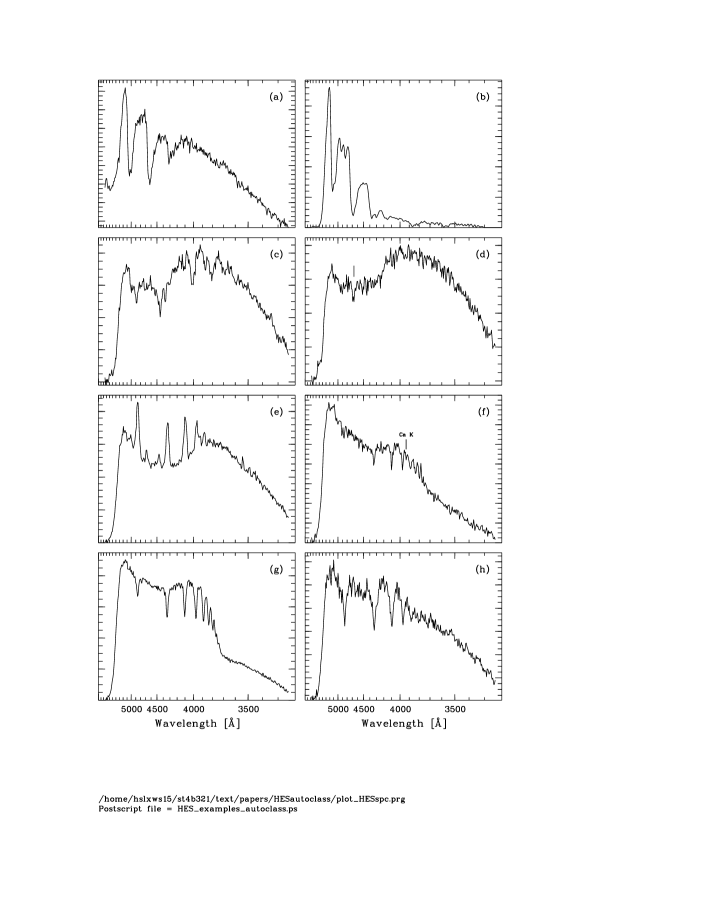
The HES (Wisotzki et al. 1996, 2000) is an objective-prism survey designed to select bright ($12.5\gtrsim B_{J}\gtrsim 17.5$) quasars in the southern extragalactic sky ($\delta<+2.5^{\circ}$; $|b|\gtrsim 30^{\circ}$). It is based on IIIa-J plates taken with the 1 m ESO Schmidt telescope and its 4^∘ prism. The plates were digitized at Hamburger Sternwarte. The HES spectra cover a wavelength range of $3200\,\mbox{\AA}<\lambda<5200\,\mbox{\AA}$ and have a seeing-limited spectral resolution of typically 15 Å at H$\gamma$ and 10 Å at Ca II K 3934 Å. This resolution makes it possible to also exploit the stellar content of the survey very efficiently. For HES example spectra see Fig. 1.

Table 2: Automatically measured spectral features in the HES. The measurement methods of the features #1–10, #17–20 and #25–27 have been described in Christlieb et al. (2001b) and Christlieb et al. (2001a). The line indices KP, GP and HP were proposed by Beers et al. (1990), and the definition of HP was later refined by Beers et al. (1999). We adapted these indices for the lower resolution of the HES spectra (in particular, the positions of some of the continuum bands were changed), and calibrated them against stars of Beers et al. present on HES plates. The $1\,\sigma$ scatters of these calibrations are $1.22$ Å, $1.41$ Å and $1.61$ Å, respectively. balmsum can be used to predict HP with an accuracy of $\sigma=1.55$ Å, and this feature is therefore superior to the directly derived HP. From the half power point distances dx_hpp1 and dx_hpp2, $U-B$ and $B-V$ colors can be derived with accuracies of better than $0.1$ mag; $c_{1}$ can be measured in HES spectra with a precission of $0.15$ mag (Christlieb et al. 2001b)

Number	Name	Description	Measurement method
#1	all5160eqw	$W_{\lambda}$ of Mg i b triplett/TiO $\lambda$ 5168	Iterative fit procedure
#2	all4861eqw	$W_{\lambda}$ of H$\beta$	Iterative fit procedure
#3	all4388eqw	$W_{\lambda}$ of Fe i $\lambda$ 4383+85	Iterative fit procedure
#4	all4340eqw	$W_{\lambda}$ of H$\gamma$	Iterative fit procedure
#5	all4300eqw	$W_{\lambda}$ of G-Band	Iterative fit procedure
#6	all4261eqw	$W_{\lambda}$ of Cr i $\lambda$ 4254 + 75 + Fe i 4260 + 72	Iterative fit procedure
#7	all4227eqw	$W_{\lambda}$ of Ca i $\lambda$ 4227	Iterative fit procedure
#8	all4102eqw	$W_{\lambda}$ of H$\delta$	Iterative fit procedure
#9	all3969eqw	$W_{\lambda}$ of Ca H + H$\epsilon$	Iterative fit procedure
#10	all3934eqw	$W_{\lambda}$ of Ca K	Iterative fit procedure
#11	balmsum	all4861eqw$+$all4340eqw$+$all4102eqw	Meta-feature
#12	CaBreak_sn	$S/N$ Calcium-break	Template matching
#13	CaBreak_cont	Contrast of Calcium-break to continuum	Template matching
#14	KP	Strength of Ca K	Ratio of average pixel values
#15	GP	Strength of G band	Ratio of average pixel values
#16	HP	Strength of H$\delta$	Ratio of average pixel values
#17	C2idx1	Strength of $\mbox{C}_{2}\;\lambda\,5165$	Ratio of average pixel values
#18	C2idx2	Strength of $\mbox{C}_{2}\;\lambda\,4737$	Ratio of average pixel values
#19	CNidx2	Strength of $\mbox{CN}\;\lambda\,4216$	Ratio of average pixel values
#20	CNidx3	Strength of $\mbox{CN}\;\lambda\,3883$	Ratio of average pixel values
#21	klcomp_1	1. continuum shape coefficient	PCA
#22	klcomp_2	2. continuum shape coefficient	PCA
#23	klcomp_3	3. continuum shape coefficient	PCA
#24	klcomp_4	4. continuum shape coefficient	PCA
#25	dx_hpp1	Half power point distance 1	Summing of pixel values
#26	dx_hpp2	Half power point distance 2	Summing of pixel values
#27	$c_{1}$	Strömgren medium band color index	Function of summed pixel values

The goals of automatic spectral classification in the HES are (a) three-dimensional classification ($T_{\mbox{\scriptsize eff}}$, $\log g$, [Fe/H]) of the total HES data base currently used for the exploitation of the stellar content, consisting of $\sim 4$ million spectra, (b) compilation of complete samples of objects of specific classes, and (c) identification of peculiar objects. These goals are similar to those emerging in DIVA and GAIA. Interesting classes of stars that can be found on HES plates include extremely metal-poor halo field stars (Christlieb & Beers 2000), field horizontal branch stars (Christlieb et al., in preparation), carbon stars (Christlieb et al. 2001a), and white dwarfs (Christlieb et al. 2001b). A large data base with spectra of known type is also very useful for cross-identification with surveys in other wavelength ranges, such as FAUST (as has been demonstrated by Brosch et al. 2000), the Two Micron All Sky Survey (2MASS), or the Deep Near Infrared Survey (DENIS). Furthermore, the data from these surveys can be used to extend the feature vectors associated with HES spectra (see below), and improve the automatic classification in the HES.

3 Automatic spectral classification

In order to achieve our classification aims, we need to construct a decision rule which allows us to assign a spectrum with feature vector $\@vec{x}$ to one of the $n_{c}$ classes $\Omega_{j}$, $j=1\dots n_{c}$, defined in the specific classification context. That is, we want to carry out a supervised classification, as opposed to unsupervised classification, where the aim is to group objects into classes not defined before the classification process. Methods of unsupervised classification and their application to HES spectra are presented in Hennig & Christlieb (2002).

3.1 Feature space

The HES data base of digital spectra can be represented by feature vectors $\@vec{x}$, consisting of a set of continuous variables $x_{i}$, i.e.

$$\@vec{x}=(x_{1},\dots,x_{d}),$$ (1)

where $d$ is the number of features used. It is critical for automatic classification to have a set of reliable features at hand. A wide range of spectral features is automatically measured in the digitized HES objective-prism spectra during the data reduction process (cf. Tab. 2): stellar absorption and emission lines, absorption bands, continuum shape including spectral breaks, bisecting points of spectral density distribution. These features are measured in unfiltered HES spectra with the methods described in Christlieb et al. (2001b).

3.2 Choosing a feature combination

It is necessary to select a subset of the available features for each classification problem, and each $S/N$ level, because of several reasons.

1. Blended lines, e.g. H$\varepsilon$+Ca H, can confuse the classification.

2. It is advantageous to exclude redundant features from the set of features used for classification, since the usage of fewer features results in more stable estimates of the parameters of the multivariate normal distributions (see Eq. (3) below).

3. The optimal feature set can vary with $S/N$. For instance, at low $S/N$ it can be useful to only use continuum shape parameters and colors for classification, because no stellar lines can be detected reliably anymore.

The evaluation of the suitability of all $2^{d}-1$ possible combinations of $d$ available features for a given classification problem is a complex task at first glance. However, it is usually possible to select a set of appropriate features by physical considerations alone. E.g., when it is desired to select metal-poor stars, only those features that are possibly useful as indicators for $T_{\mbox{\scriptsize eff}}$, $\log g$, [Fe/H], and [C/Fe] need to be considered. By means of accuracy considerations and parameter studies, further features can be rejected. Finally, it is also possible to reduce the dimensionality of the feature space by a priori combining redundant features, e.g. the equivalent widths of the Balmer lines to a sum of equivalent widths. The remaining set of features is then evaluated with the methods described in Sect. 4.1.

3.3 Learning sample

For supervised classification, a learning sample is needed. For our purposes, we define a learning sample to be a set of $n_{l}$ objects for which the feature vectors are known,

$$\{\@vec{x}\}=(\@vec{x}_{1},\dots,\@vec{x}_{n_{l}}),$$ (2)

and for which it is known to what class they belong. These classes can be defined, e.g., by grouping a set of objects according to their stellar parameters (e.g. $T_{\mbox{\scriptsize eff}}$, $\log g$, [Fe/H]), or by manually assigning classes to a set of spectra by comparison with reference objects. With the help of a learning sample, information on the class-conditional probability densities $p(\@vec{x}|\Omega_{j})$ can be gained. $p(\@vec{x}|\Omega_{j})d\!\@vec{x}$ is the probability to observe a feature vector in the range $\@vec{x}\dots\@vec{x}+d\!\@vec{x}$ in the class $\Omega_{j}$. We inspected the one-dimensional class-conditional probability distributions of the classes covered by the learning samples used in this work, and qualitatively found their shapes to agree well with Gaussians. We hence model $p(\@vec{x}|\Omega_{j})$ by multivariate normal distributions, i.e.,

$${\small p(\@vec{x}|\Omega_{j})=\frac{1}{(2\pi)^{d/2}\sqrt{|\Sigma_{j}|}}\exp\left\{-\frac{1}{2}\left(\@vec{x}-\@vec{\mu}_{j}\right)^{\prime}\Sigma^{-1}_{j}\left(\@vec{x}-\@vec{\mu}_{j}\right)\right\},}$$ (3)

where $j$ denotes class number, $\@vec{\mu}_{j}$ the mean feature vector of class $\Omega_{j}$, and $\Sigma_{j}$ the covariance matrix of class $\Omega_{j}$.

3.4 Decision rules

A central issue in automatic classification is the construction of a decision rule which is optimal for the given classification problem. In the HES, we use three decision rules: the Bayes rule, a minimum cost rule, and a rejection rule.

3.4.1 Bayes’ rule

Classification with Bayes’ rule minimizes the total number of misclassifications, if the true distribution of class-conditional probabilities $p(\@vec{x}|\Omega_{i})$ is used (Hand 1981; Anderson 1984). Using Bayes’ theorem,

$$P(\Omega_{i}|\@vec{x})=\frac{P(\Omega_{i})p(\@vec{x}|\Omega_{i})}{\sum\limits_{\forall i}P(\Omega_{i})p(\@vec{x}|\Omega_{i})},$$ (4)

posterior probabilities $P(\Omega_{i}|\@vec{x})$ can be calculated. A spectrum of unknown class, with given feature vector $\@vec{x}$, can then be classified using Bayes’ rule:

Bayes’ rule:

Assign a spectrum with feature vector $\@vec{x}$ to the class with the highest posterior probability $P(\Omega_{i}|\@vec{x})$.

3.4.2 Minimum cost rule

In most of the classification problems arising in the HES it is desired to gather a sample of objects of a specific class, or a specific set of classes. In these cases, Bayes’ rule is not appropriate, because we do not want to minimize the total number of misclassifications, but the misclassifications between the desired class(es) of objects, and the remaining classes. Suppose we have three classes, A-, F-, and G-type stars, and we want to gather a complete sample of A-type stars. Then only misclassifications between A-type stars and F- and G-type stars (and vice versa) are of interest. More specifically, misclassifications of A-type stars to F- and G-type stars (leading to incompleteness) are least desirable when a complete sample shall be gathered, and erroneous classification of F- and G-type stars as A-type stars (resulting in sample contamination) can be accepted at a moderate rate. Misclassifications between F- and G-type stars can be totally ignored, because the target object type is not involved.

Classification aims like this can be realized by using a minimum cost rule. Cost factors $r_{hk}$, with

$$0\leq r_{hk}\leq 1;\qquad h=1,\dots,n_{c};\quad k=1,\dots,n_{c}.$$ (5)

allow to assign relative weights to individual types of misclassifications. The cost factor $r_{hk}$ is the relative weight of a misclassification from class $\Omega_{h}$ to class $\Omega_{k}$.

Suppose we have an object of unknown class, with feature vector $\@vec{x}$. We ask how large the cost is if it belongs to class $\Omega_{h}$, and would be assigned to class $\Omega_{k}$, $h\not=k$. The cost $C_{h\to k}(\@vec{x})$ is:

$$C_{h\to k}(\@vec{x}) = r_{hk}P(\Omega_{h}|\@vec{x})$$ (6)

$$= r_{hk}\frac{P(\Omega_{h})\,p(\@vec{x}|\Omega_{h})}{\sum\limits_{i=1}^{m}P(\Omega_{i})\,p(\@vec{x}|\Omega_{i})}$$

$$= r_{hk}\frac{a_{h}p_{h}(\@vec{x})}{\sum\limits_{i=1}^{m}a_{i}p_{i}(\@vec{x})}.$$

In the last step we have used the abbreviations $P(\Omega_{h})=a_{h}$ and $p(\@vec{x}|\Omega_{h})=p_{h}(\@vec{x})$. We do not know to which of the possible classes $\Omega_{h}$, $h=1,\dots,n_{c}$, the object actually belongs. Therefore, we estimate the expected cost $C_{k}(\@vec{x})$ for assigning an object with feature vector $\@vec{x}$ to the class $\Omega_{k}$ by computing the following sum of costs:

$$C_{k}(\@vec{x}) = \sum\limits_{h=1\atop h\not=k}^{m}C_{h\to k}(\@vec{x})$$ (7)

$$= \sum\limits_{h=1\atop h\not=k}^{m}r_{hk}\frac{a_{h}p_{h}(\@vec{x})}{\sum_{i=1}^{m}a_{i}p_{i}(\@vec{x})}$$

Now we can formulate the minimum cost rule, which minimizes the total cost (Hand 1981).

Minimum Cost Rule:

Assign an object with feature vector $\@vec{x}$ to the class $\Omega_{k}$ with the lowest expected cost $C_{k}(\@vec{x})$.

If the cost factors are chosen such that $r_{hk}\equiv\delta_{hk}$, the minimum cost rule classification is identical to classification using Bayes’ rule. In this case the cost for assigning the class $\Omega_{k}$ to a spectrum with feature vector $\@vec{x}$ is the probability that the object belongs to one of the other classes $h\not=k$. This follows immediately from Eq. (7). If $r_{hk}\not=\delta_{hk}$, the total number of misclassifications is not minimized, so that the quality of a minimum cost rule classification has to be evaluated by other criteria.

For any given classification aim, one can divide the cost factors to be chosen into three sets:

t2o:

Cost factor for misclassification of an object of the target class (‘t’) to (‘2’) one of the other classes (‘o’).

o2t:

Cost factor for contamination of the target class.

o2o:

Cost factor for misclassification between other classes.

Since sample completeness and contamination are interdependent, in practice only the relative value t2o/o2t has to be adjusted. For this purpose, the classification results as a function of t2o/o2t are evaluated. The expected error rates, estimated e.g. with the “leaving one out” method (see Sect. 4.1 below), tell which level of completeness and sample contamination will be achieved. Christlieb et al. (1998) presented a software tool for a convenient choice of cost factors.

3.4.3 Rejection rule

Non-mathematically speaking, Bayes’ rule assigns the class with the highest relative resemblance to each spectrum to be classified. However, it is ignorant of the absolute resemblance: A spectrum with feature vector $\@vec{x}$ may be assigned to a class with very low posterior probability $p(\Omega_{i}|\@vec{x})$, if $p(\Omega_{i}|\@vec{x})$ is even lower for all other classes. This means that a class is assigned to all spectra, even to “garbage spectra” which are disturbed, for instance, by plate artifacts. Therefore, it is useful to apply a rejection rule in addition to either the Bayes rule or the minimum cost rule. The rejection rule can also be used “stand alone” for the identification of peculiar objects, e.g., quasars.

Rejection rule:

Reject an object from classification to class $\Omega_{i}$, if $A(\Omega_{i};\@vec{x})>\beta\,$.

The parameter $\beta$ is a threshold to be chosen, and the parameter $A$ is the atypicality index suggested by Aitchison et al. (1977),

$$A(\Omega_{i},\@vec{x})=\Gamma\left\{\frac{d}{2};\frac{1}{2}\left(\@vec{x}-\@vec{\mu}_{i}\right)^{\prime}\Sigma^{-1}_{i}\left(\@vec{x}-\@vec{\mu}_{i}\right)\right\},$$ (8)

where $\Gamma(a;x)$ is the incomplete gamma function and $d$ the number of features used for classification. Use of the above rejection criterion is identical to performing a $\chi^{2}$ test of the null hypothesis $H_{0}$ that an object with feature vector $\@vec{x}$ belongs to class $\Omega_{i}$ at significance level $1-\beta$, against the alternative hypothesis $H_{1}$ that it does belong to class $\Omega_{i}$. We reject the null hypothesis if its significance level is low, i.e., if it is very unlikely that a feature vector $\@vec{x}$ is observed for class $\Omega_{i}$, given the multivariate normal distributions (3) are the true distributions of the class-conditional probabilities $p(\@vec{x}|\Omega_{i})$.

4 Classification performance

Figure 2: Distribution of the three features used for classification of main sequence turnoff stars in one learning sample class, and for different signal-to-noise ratios.

In a first application of automatic spectral classification in the HES, we selected candidates for extremely metal-poor halo field stars. Christlieb (2000) and Christlieb & Beers (2000) have shown that with this method, a very efficient selection of metal-poor stars is feasible. 80 % of an investigated sample of 56 highest priority metal-poor candidates were shown by medium-resolution follow-up spectroscopy to have metallicities below $-2.0$ dex, and results based on a larger sample of stars, including also fainter and lower priority candidates, indicate that the overall efficiency for the selection of stars with $\mbox{[Fe/H]}<-2.0$ is $\sim 60$ % in the HES (Christlieb et al., in preparation). This is the most efficient selection of metal-poor stars ever obtained in a wide-angle survey for such stars. In this paper we focus on results of a systematic investigation of the classification performance for stars in the effective temperature range $5200\,\mbox{K}<T_{\mbox{\scriptsize eff}}<6800\,\mbox{K}$ achievable in the HES, by means of a simulation study.

4.1 Evaluation of classification rules

Classification rules can be evaluated by the number of expected misclassifications (in the case of Bayes’ rule), or by the total expected cost (in the case of the minimum cost rule). The three most important methods to estimate these numbers are (Deichsel & Trampisch 1985):

1. Re-substitution

2. “Hold out” method

3. “Leaving one out” method.

Re-substitution means that one uses the learning sample also as test sample. The drawback of this method is that one underestimates the number of expected misclassifications, because a classification rule derived with the help of a finite learning sample is always adapted to the individual composition of the learning sample. Therefore, the estimation of the expected number of misclassifications is biased (Deichsel & Trampisch 1985).

An improvement in this respect is gained when the “hold out” method is used. Here one randomly divides the learning sample disjointly into a new, smaller learning sample, and a test sample. Since the learning sample and test sample are completely independent in this case, an unbiased estimate of the expected error rates is possible (Deichsel & Trampisch 1985). However, the drawback is that one needs a large enough learning sample. When modeling the class-conditional probabilities with multivariate normal distributions, the learning sample size has to be large enough to ensure a robust estimation of the parameters of the distributions.

The problem of learning sample size can be circumvented by using the “leaving one out” method. Suppose we have a learning sample of size $n_{l}$. We exclude object $i$ from the learning sample, and construct the classification rule using the $n_{l}-1$ remaining objects. Object $i$ is then classified with this classification rule. This procedure is repeated $n_{l}$ times, so that each object of the learning sample is excluded once, and used as test sample. By adding up the numbers of misclassifications obtained in each step, one gets an unbiased estimate of the expected error rate (Deichsel & Trampisch 1985). The only drawback of this method is that it consumes a lot more computing time than the previously mentioned methods, since $n_{l}$ classification rules have to be constructed. However, the computing time increases only linearly with learning sample size $n_{l}$, so that the usage of the “leaving one out” method was feasible for all HES learning samples used so far (the largest learning sample used had $n_{l}=165\,000$).

4.2 Simulation study on the classification performance in the HES

For our simulation study, we employed a grid of model spectra converted to objective prism spectra with the methods described in Christlieb et al. (2001b). The grid covers the following stellar parameter range:

$$T_{\mbox{\scriptsize eff}} = 5200(200)6800\,\mbox{K}$$

$$\log g = 2.2(0.8)4.6$$

$$\left[\mbox{Fe/H}\right] = -0.3,-0.9,-1.5(0.3)-3.6$$

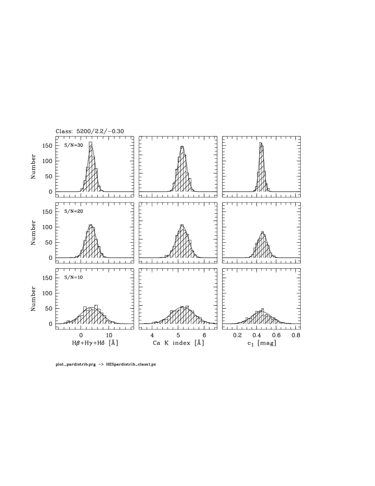
The values in brackets refer to grid point distances. The grid defines 360 classes. Since it is one of the aims of our simulation study to investigate how the classification accuracy changes with $S/N$, we need to simulate spectra of different $S/N$. For this, we added Gaussian noise to the grid of simulated spectra so that spectra with $S/N=5(5)30$ resulted. The adequatness of this noise model for HES spectra has been demonstrated by Christlieb et al. (2001b). It is necessary to produce learning samples for different $S/N$ levels because the width of the class-conditional probability distributions change with $S/N$ (see Fig. 2). We then performed a Bayes classification, using the three features $c_{1}$, balmsum (the sum of the equivalent widths of H$\beta$, H$\gamma$ and H$\delta$), and the Ca K index KP. This feature set was found to be best suitable for the desired three-dimensional classification in parameter studies, and by systematic evaluation of the classification performance of different feature combinations.

For each spectral class 500 simulated spectra were computed, which is a large enough number to randomly subdivide the grid into a learning sample and an independent test sample. To obtain a realistic estimate of the classification performance, two effects have to be taken into account:

Undersampling of the error distribution:

In our simulation study, we use a grid of stellar parameters. Therefore, if a classification error is smaller than half of the grid point distance, an error of zero is measured. Therefore, the classification error is systematically underestimated in these cases.

Discretization error:

Real samples of stars have a continuous distribution of stellar parameters. These parameters will be mapped to our discrete grid. This results in classification errors for stars having stellar parameters lying between two grid points.

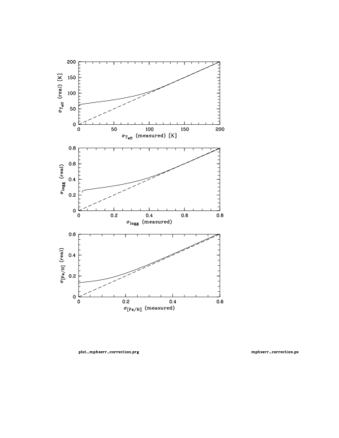
We have taken these effects into account by applying (upward) corrections to the classification errors measured on our model spectra grid (see Fig. 3). For the estimation of the corrections for error distribution undersampling, Gaussian random errors were added to the grid point parameters to simulate classification errors, and the measured errors were compared with the errors known from the chosen $\sigma$ of the Gaussian distribution. The discretization error correction to be applied was derived by mapping continuously distributed stellar parameters to our grid, and computing the mean difference between real parameters and the parameters detected by the grid.

Figure 3: Corrections applied to the classification errors measured in the simulation study. For explanation see text

In the stellar parameter range we explored so far, the corrected accuracy in effective temperature classification is better than 400 K for spectra with $S/N>10$, which typically corresponds to $B_{J}<16.5$ (see Christlieb et al. 2001b). The accuracies in $\log g$ and [Fe/H] are better than $0.68$ dex for the same magnitude range. Note that the accuracy in [Fe/H] strongly depends on [Fe/H] itself, since the Ca K line, used as metallicity indicator, is not detectable in the spectra of the lowest metallicity turnoff stars at the spectral resolution of the HES. Therefore, a metallicity classification is not possible in that part of the stellar parameter space, resulting in a larger average classification error.

Figure 4: Classification precision for stars in the effective temperature range $5200\,\mbox{K}<T_{\mbox{\scriptsize eff}}<6800\,\mbox{K}$ in the HES as a function of $S/N$, as obtained with Bayes classification in our simulation study

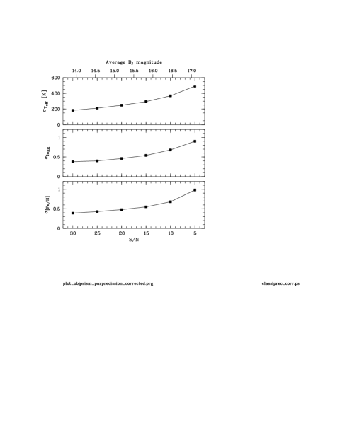
As a plausibility check we compared our results with the classification accuracies we would expect from simple, one-dimensional parameterization approaches using $B-V$, $c_{1}$ and KP as temperature, gravity and metallicity indicators, respectively. In the effective temperature range $5200\,\mbox{K}<T_{\mbox{\scriptsize eff}}<6800\,\mbox{K}$, $\Delta(B-V)/\Delta T_{\mbox{\scriptsize eff}}\sim 0.028\,\mbox{mag}/100\,\mbox{K}$ (Lang 1992). The average accuracy of the HES $B-V$ calibration in the temperature range under consideration, averaged over the full magnitude range covered by the HES, is $\sigma_{B-V}=0.07$ mag (Christlieb et al. 2001b), so that an average temperature classification accuracy of $\sigma_{T_{\mbox{\tiny eff}}}=260$ K is expected. This is consistent with classification errors of 200–420 K in the magnitude range $14.0<B_{J}<17.5$. $\Delta c_{1}/\Delta\log g\sim 0.1$–$0.3\,\mbox{mag}/\mbox{dex}$ in the effective temperature range under consideration (Lang 1992). The average accuracy of the HES $c_{1}$ calibration is $\sigma_{c_{1}}=0.15$ mag (Christlieb et al. 2001b), so that we expect a gravity classification precision of $\sigma_{\log g}=0.5$–1.5 dex. This is consistent with $\sigma_{\log g}<0.68$ measured in our simulation. Finally, from Fig. 4 of Beers et al. (1990) one can read that at $B-V=0.5$, the difference in the Ca K index KP between a star of $\mbox{[Fe/H]}=-2.0$ and a star of $\mbox{[Fe/H]}=-3.0$ is $2.7$ Å and $4.7$ Å for dwarfs and giants, respectively. Considering the fact that $\sigma_{\mbox{\scriptsize\tt KP}}=1.22$ Å in the HES, it is not surprising that classification precisions as high as $0.4$ dex can be achieved for the brightest stars in the HES (see Fig. 4).

5 Discussion and conclusions

We have demonstrated that automatic spectral classification of turnoff stars, using “classical” statistical methods, is feasible in the HES with high accuracy. Our results suggest that it might be possible to determine the metallicity distribution function (MDF) of the galactic halo directly from a large sample of HES spectra. The MDF is an important constraint for models of galactic chemical evolution (see, e.g., Ikuta & Arimoto 1999; Oey 2000).

The described methods are currently being applied to the large HES data base of digital spectra, in order to select interesting stellar objects in an automated fashion, and fully exploit the large scientific potential present in our data base.

Our algorithms can easily be adapted for automatic classification of other large data sets, e.g. those to be compiled by the DIVA and GAIA missions.