Probing the mass loss history of carbon stars using CO line and dust continuum emission

An extensive modelling of CO line emission from the circumstellar envelopes around a number of carbon stars is performed. By combining radio observations and infrared observations obtained by ISO the circumstellar envelope characteristics are probed over a large radial range. In the radiative transfer analysis the observational data are consistently reproduced assuming a spherically symmetric and smooth wind expanding at a constant velocity. The combined data set gives better determined envelope parameters, and puts constraints on the mass loss history of these carbon stars. The importance of dust in the excitation of CO is addressed using a radiative transfer analysis of the observed continuum emission, and it is found to have only minor effects on the derived line intensities. The analysis of the dust emission also puts further constraints on the mass loss rate history. The stars presented here are not likely to have experienced any drastic long-term mass loss rate modulations, at least less than a factor of $\sim$5, over the past thousands of years. Only three, out of nine, carbon stars were observed long enough by ISO to allow a detection of CO far-infrared rotational lines.

1 Introduction

Mass loss is associated with many phases of stellar evolution. It is of particular importance during the final evolutionary stage of low to intermediate mass stars, the asymptotic giant branch (AGB), when it increases dramatically. Its overall characteristics, e.g., magnitude, geometry, and kinematics, are reasonably well established, but to what extent such effects as asymmetry, non-homogeneity, temporal variability, etc., are important is not known. During the AGB-phase, stars in the mass range about 1.5–4 M_☉ and with ’normal’ chemical compositions start to evolve into carbon stars, i.e., stars with more carbon than oxygen in their atmospheres, through the dredge-up of freshly synthesized carbon in He-shell flashes (Straniero et al. 1997; Busso et al. 1999). It appears that all AGB carbon stars are losing mass at a rate in excess of 10^-8 M_☉ yr^-1 (Olofsson et al. 1993; Schöier & Olofsson 2001).

Approximately 10% of all carbon stars appear to have been subject to drastic changes in their mass loss rates over relatively short periods of time (a few thousand years). Most notable are the CO radio line observations of detached circumstellar envelopes (Olofsson et al. 1996, 2000; Lindqvist et al. 1999; Schöier & Olofsson 2001). The time interval between these, supposedly reoccuring, mass ejections is estimated to be about 10⁵ years, and they are possibly linked with the He-shell flashes predicted to occur in carbon stars (Olofsson et al. 1990; Schröder et al. 1999; Steffen & Schönberner 2000). Less dramatic mass loss rate modulations have recently been observed by Mauron & Huggins (1999, 2000) in the form of a multiple-shell structure around the high mass loss rate carbon star CW Leo (or IRC+10216). This suggests an isotropic mass loss mechanism with a variability on a broad range of, relatively short, time scales $\sim$40$-$800 yr. Moreover, spatially resolved interferometric CO millimetre observations currently have the potential to trace mass loss rate modulations on the order of a factor 2$-$3 down to a time scale of several hundred years (Bieging & Wilson 2001). For changes of the mass loss rate over longer periods of time, $\gtrsim$10⁵ yr, statistical studies are generally required. The emerging picture is that of a mass loss rate which increases gradually with time during the AGB evolution, and its maximum attainable value depends on the initial main-sequence mass (Habing 1996). Observational results like these are crucial for the understanding of mass loss during late stellar evolution, and for the possibility to pinpoint the mechanism(s) behind this phenomenon, which determines the time scale during the final evolutionary AGB-stage.

Table 1: Stellar and circumstellar properties of the sample stars.

			$D$	$L_{*}$	$\dot{M}$d	$v_{\mathrm{e}}$	$r_{\mathrm{p}}$e	$h$f
Sourcea	Alt. nameb	Var. typec	[pc]	[L☉]	[M☉yr-1]	[km s-1]	[cm]
V384 Per		Mira	560	8100	3.5$\times$10-6	15.0	1.4$\times$1017	0.4
CW Leo	IRC+10216	Mira	120	9600	1.5$\times$10-5	14.5	3.7$\times$1017	1.0
RW LMi	CIT 6	SRa	440	9700	6.0$\times$10-6	17.0	1.9$\times$1017	1.4
Y CVn		SRb	220	4400	1.5$\times$10-7	08.5	2.9$\times$1016	0.2
IRAS 15194-5115		Mira:	600	8800	1.0$\times$10-5	21.5	3.2$\times$1017	1.5
V Cyg		Mira	370	6200	1.2$\times$10-6	11.5	8.5$\times$1016	1.2
S Cep		Mira	340	7300	1.5$\times$10-6	22.0	7.5$\times$1016	0.4
AFGL 3068		Mira:	820	7800	1.5$\times$10-5	14.0	3.8$\times$1017	1.5
LP And	IRC+40540	Mira	630	9400	1.5$\times$10-5	14.0	3.8$\times$1017	0.7

^a Parameters taken from Schöier & Olofsson (2001) except for IRAS 15194-5115 and AFGL 3068 which are presented in Ryde et al. (1999) and Woods et al. (in prep.), respectively.
^b Other frequently used name.
^c A colon (:) indicates uncertain classification.
^d A CO abundance of 1.0$\times$10^-3 relative to H₂ was assumed in deriving the mass loss rates.
^e Estimated CO photodissociation radius.
^f Dust-grain heating parameter (see text for details).

Carbon monoxide, CO, is a good tracer of the molecular gas content, and it has been extensively used to determine the properties of the circumstellar envelopes (CSEs) formed by the mass loss, e.g., recently Schöier & Olofsson (2001) used CO millimeter line observations and a detailed modelling of the emission to determine mass loss rates for a large sample of optically bright carbon stars. The Infrared Space Observatory (ISO; Kessler et al. (1996)) opened a new window for observing AGB-stars, allowing studies of molecular gas, in their expanding CSEs, much closer to the central stars than was previously possible using mainly ground based radio telescopes (Cernicharo et al. 1996; Ryde et al. 1999). As an example Ryde et al. (1999) studied the high mass loss rate carbon star IRAS 15194-5115 in several rotational transitions in the ground vibrational states of ¹²CO and ¹³CO. In this way different radial regions of the CSE were probed, and constraints on the temporal changes in the wind characteristics, in particular the mass loss rate, were obtained.

In this paper the method used by Ryde et al. (1999) is adopted in a study of a number of carbon stars observed by ISO. The radiative transfer analysis is further extended to include also the stellar light reemitted by the surrounding dust, and to investigate its effect on the excitation of CO.

Figure 1: The FIR spectrum of RW LMi, as observed by ISO, showing CO rotational lines in emission superimposed on the continuum emitted by the dust present around the star. All rotational transitions within the ground vibrational state in this wavelength region (from $J$$=$14$\rightarrow$13 to $J$$=$29$\rightarrow$28) are indicated. In addition, the interstellar [CII] line is marked.

2 Observations

Our sample consists of nine carbon stars, of which seven were included in the large CO radio line survey of carbon stars made by Olofsson et al. (1993) [see also Schöier & Olofsson (2001) for additional CO observations]. The CO data on IRAS 15194-5115 and AFGL 3068 are presented in Ryde et al. (1999) and Nyman et al. (in prep.), respectively. Some of the stellar properties of the sample sources, as well as the results from detailed radiative transfer modelling of the CO data [Schöier & Olofsson (2001); Ryde et al. (1999); Woods et al. (in prep.)], are listed in Table 1.

The FIR data were retrieved from the ISO data archive. The observations were carried out with the Long Wavelength Spectrometer (LWS, Clegg et al. 1996), which had a field of view on the sky of 84$\arcsec\times$84$\arcsec$. The spectrometer was used in the grating mode (LWS01), covering the range 90$-$197 $\mu$m, which provided a mean spectral resolution element of $\sim$0.7 $\mu$m. Since this corresponds to R$=$$\lambda/\Delta\lambda$$\sim$100$-$250, the circumstellar lines are far from being resolved. In what follows, only the line-integrated flux will be discussed, since no kinematic information is available. The spectra were sampled at 0.15 $\mu$m.

The data reduction was made using the pipeline basic reduction package OLP (v. 9.5) and the ISO Spectral Analysis Package (ISAP v. 2.0). The pipeline processing of the data, such as wavelength and flux calibration, is described in Swinyard et al. (1996); the combined absolute and systematic uncertainties in the fluxes are on the order of $\pm$15–20%. The accuracy of the wavelength varies and can be as bad as $\pm$0.1 $\mu$m. The integrated intensities of the emission lines are measured in the same manner as in Ryde et al. (1999), i.e., a dust continuum level is estimated and subtracted over a limited wavelength interval, usually $\sim$10 $\mu$m. This procedure introduces additional, sometimes large, uncertainties in the line fluxes. The errors in the fluxes due to the uncertain continuum subtraction are, on the average, estimated to be of the same order as the calibration uncertainties. A total error of $\pm$25% in the measured line fluxes is assumed for all stars. In the radiative transfer modelling of the CO emission lines observed by ISO the quality of the fits are good (see Sect. 5), with reduced $\chi^{2}$ values $\sim$1, indicating that the errors assigned to the fluxes are reasonable.

The final LWS spectra are dominated by thermal radiation due to the dust present around these objects. Superimposed on the dust continuum are molecular emission lines, of which ¹²CO, ¹³CO, and H¹²CN lines have been identified in the LWS spectra of CW Leo (Cernicharo et al. 1996) and IRAS 15194-5115 (Ryde et al. 1999). The LWS spectrum of RW LMi, where only emission lines arising from ¹²CO have been identified, is presented in Fig. 1. The observed fluxes are presented in Tables 2$-$4. For the rest of the sample stars presented in Table 1 only upper limits to the CO FIR line emission were obtained, Table 6.

3 Molecular line radiative transfer

In this section our standard model adopted for the excitation analysis of the observed CO rotational line emission is presented (Schöier & Olofsson 2001). An expansion of the standard model is made to include a dust component, and its effect on the CO excitation is investigated.

3.1 The standard model

The observed circumstellar CO line emission is modelled using a numerical simulation code based on the Monte Carlo method. The code solves the non-LTE radiative transfer problem of CO taking into account 50 rotational levels in each of the fundamental and first excited vibrational states. The CSE is assumed to be spherically symmetric and to expand at a constant velocity. The code simultaneously solves the energy balance and statistical equilibrium equations allowing for a self-consistent treatment of CO line cooling. After convergence is reached in the level populations the radiative transfer equation is solved exactly for the transitions of interest. The resulting brightness distributions are subsequently convolved with the appropriate beams to allow a direct comparison with the observational data. See Schöier (2000) and Schöier & Olofsson (2001) for details on the radiative transfer. The code has been tested against other radiative transfer codes for a set of benchmark problems to a high accuracy (van Zadelhoff et al. 2002).

The recently published collisional rates of CO with H₂ by Flower (2001) have been adopted assuming an ortho-to-para ratio of 3. For temperatures above 400 K the rates from Schinke et al. (1985) were used and further extrapolated to include transitions up to $J$$=$50. The collisional rates adopted here differ from those used in the previous modelling of these sources (Ryde et al. 1999; Schöier & Olofsson 2001) and accounts for the slightly different envelope parameters derived in the present analysis.

The size of the CO envelope was fixed to 4$\times$10¹⁷ cm and 2$\times$10¹⁷ cm for CW Leo and RW LMi, respectively. The adopted sizes reproduce the extents of the CO($J$$=$1$\rightarrow$0) emission as mapped by the IRAM PdB interferometer for these two sources (Neri et al. 1998). The radial brightness distribution of the CO($J$$=$1$\rightarrow$0) emission towards RW LMi shows signs of a second, weak and more extended, component possibly produced by a modulation of the mass loss rate (Schöier & Olofsson 2001). Inclusion of this component in the modelling only marginally affects the derived CO($J$$=$1$\rightarrow$0) line intensities. Transitions involving higher $J$-levels are unaffected and this second component is not further considered here. For IRAS 15194-5115 no interferometric observations exist at present and the, marginally resolved, CO($J$$=$1$\rightarrow$0) single-dish map presented by Nyman et al. (1993) was used. A CO envelope size of $\sim$2$\times$10¹⁷ cm, reproduces the observed radial brightness distribution well. In the parameter space investigated here only the CO($J$$=$1$\rightarrow$0) line intensity is sensitive to the adopted envelope size. However, the effect is generally weak (Schöier & Olofsson 2001).

The standard model includes radiation from a central source approximated by one or two blackbodies located within the assumed inner radius of the model CSE. Here we assume that each central source is described by a single blackbody of the luminosity listed in Table 1 and with a temperature of 2200 K. For the majority of the sample stars, which have dense CSEs, the line intensities derived from the model are not sensitive to the adopted description of the stellar spectrum due to the high line optical depths. The stellar photons are typically absorbed within the first few shells in the model. Thermal emission from the dust present in the CSE, and the increase of total optical depth at the line wavelengths, is not properly treated in the scheme of the standard model. Dust emission has the potential of affecting the level populations in the ground vibrational state, in particular through pumping via excited vibrational states. How this is incorporated into the Monte Carlo method is described in Sect. 3.2, and its importance for the CO excitation is discussed in Sect. 5.3.

In order to put constraints on possible mass loss rate modulations in the sources where CO line emission is detected by ISO (i.e., CW Leo, RW LMi, and IRAS 15194-5115), the two adjustable parameters in the radiative transfer analysis, the mass loss rate and the $h$-parameter, are varied. The $h$-parameter is defined as,

$$h=\left(\frac{\Psi}{0.01}\right)\left(\frac{2.0\,\mathrm{g\,cm}^{-3}}{\rho_{\mathrm{gr}}}\right)\left(\frac{0.05\,\mu{\mathrm{m}}}{a_{\mathrm{gr}}}\right),$$ (1)

where $\Psi$ is the dust-to-gas mass loss rate ratio, $\rho_{\mathrm{gr}}$ the mass density of a dust grain, and $a_{\mathrm{gr}}$ the size of a dust grain. The normalized values are the ones used by Schöier & Olofsson (2001) to fit the CO millimetre and sub-millimetre line emission of CW Leo using the standard model, i.e., $h$$=$1 for this object. The $h$-parameter enters into the expression for the heating term due to the momentum transfer from dust to gas

$$H_{\mathrm{dg}}=\frac{3}{8}\rho_{\mathrm{H}_{2}}\frac{\Psi}{a_{\mathrm{gr}}\rho_{\mathrm{gr}}}\frac{{v_{\mathrm{dr}}^{3}}}{1+\frac{v_{\mathrm{dr}}}{v_{\mathrm{e}}}},$$ (2)

where $\rho_{\mathrm{H}_{2}}$ is the density of molecular hydrogen and $v_{\mathrm{dr}}$ is the drift velocity between the dust and the gas. The drift velocity is expressed by [see Schöier & Olofsson (2001) and references therein]

$$v_{\mathrm{dr}}=v_{\mathrm{d}}-v_{\mathrm{e}}=\left(\frac{Lv_{\mathrm{e}}Q}{\dot{M}c}\right)^{1/2},$$ (3)

where $Q$ is the flux averaged momentum transfer efficiency of the dust assumed to have a value of 0.03 (Schöier & Olofsson 2001). This is the dominant heating process in the CSE, and it is therefore important in determining the kinetic temperature of the gas.

The best fit model is found by minimizing the chi-squared statistic

$$\chi^{2}=\sum^{N}_{i=1}\left[\frac{(F_{\mathrm{mod},i}-F_{\mathrm{obs},i})}{\sigma_{i}}\right]^{2},$$ (4)

where $F$ is the flux and $\sigma_{i}$ the uncertainty in the measured flux of line $i$, and the summation is done over all $N$ independent observations. In the $\chi^{2}$-analysis the ISO fluxes are assumed to be accurate to within 25%. The millimetre observations are better calibrated with an estimated uncertainty within 15% for these strong CO sources, which are often used as standard sources at radio telescopes.

3.2 Addition of a dust component

The addition of a dust component in the Monte Carlo scheme is straightforward. Scattering is of no importance at the wavelengths of interest here, and only emission and absorption by the dust particles are considered. The dust is assumed to be closely coupled to the radiation locally, and the particles emit thermal radiation, described by the dust temperature $T_{\mathrm{d}}(r)$, according to Kirchhoff’s law. The number of model photons emitted per second by the dust within a small volume of the envelope, ${\Delta}V$, and over a small frequency interval, $\Delta\nu$, can then be written as

$$N_{\mathrm{d}}(r)=\frac{4\pi}{h\nu}\kappa_{\nu}\rho_{\mathrm{d}}(r)B_{\nu}[T_{\mathrm{d}}(r)]{\Delta}V(r)\Delta\nu,$$ (5)

where $\kappa_{\nu}$ is the dust opacity per unit mass, $\rho_{\mathrm{d}}$ the dust mass density, and $B_{\nu}$ the Planck function. Typically the frequency passband is $\sim$3$\times$$v_{\mathrm{e}}$ and centered on the line rest frequency $\nu_{0}$. The dust temperature structure is obtained from the detailed dust radiative transfer modelling described in Sect. 4. The model photons emitted by the dust are released together with the other model photons. The additional opacity provided by the dust, Eq. 6, is added to the line optical depth.

Moreover, since, in general, the dust and the gas have different temperatures heat will be exchanged during a collision. The treatment of this process, which has implications only for the gas, is adopted from Groenewegen (1994) and it is included as an extra heating/cooling term in the energy balance equation solved during each iteration by the radiative transfer code.

4 Dust radiative transfer

The FIR spectra of carbon stars generally show bright thermal radiation due to the large quantity of dust present in the CSEs around these objects, which absorb and re-emit the stellar visible and near-infrared radiation. Dust emission is potentially important for excitation of vibrationally excited states in molecules. This may affect the level populations in the ground vibrational state, whose rotational lines are most often used to constrain circumstellar models. In the case of CO the first excited vibrational state lies at 4.6 $\mu$m, i.e., close to the peak of the spectral energy distribution (SED; see Fig. 5). A shortcoming of our standard model of radiative transfer in molecular lines is the lack of a full treatment of the radiative transfer of the dust. The gas has no importance for the radiative transfer of the dust, which allows the dust analysis to be carried out separately in order to determine, in particular, the dust temperature structure needed for the more detailed molecular excitation analysis.

Figure 2: $\chi^{2}$-maps showing the sensitivity of the CO radiative transfer model, using the observed integrated intensities as constraints, to the mass loss rate and the $h$-parameter. Contours are drawn at the 1, 2 and 3$\sigma$ levels. The number of observational constraints, $N$, are also given. The quality of the best fit models are very good as determined from their reduced chi-squared statistics, $\chi^{2}_{\mathrm{red}}$ $\sim$1.

4.1 Dust modelling

The radiative transfer problem in a dusty CSE possesses scaling properties (Ivezić & Elitzur 1997). This fact is put to use in the publicly available radiative transfer code DUSTY (Ivezić et al. 1999), which is adopted here to model the observed continuum emission.

The most important parameter in the dust radiative transfer modelling is the dust optical depth

$$\tau_{\lambda}=\kappa_{\lambda}\int^{r_{\mathrm{e}}}_{r_{\mathrm{i}}}\rho_{\mathrm{d}}(r)dr,$$ (6)

where the integration is performed from the inner ($r_{\mathrm{i}}$) to the outer ($r_{\mathrm{e}}$) radius of the CSE. The dust is assumed to have fully condensated at the inner radius of the model CSE.

In the dust modelling the same basic assumptions are made as for the gas modelling, i.e., a spherically symmetric envelope expanding at a constant velocity. This results in a dust density structure where $\rho_{\mathrm{d}}$$\propto$$r^{-2}$. Amorphous carbon dust grains with the optical constants given in Suh (2000) are adopted. The properties of these grains were shown to reasonably well reproduce the SEDs in a sample of carbon stars. For simplicity, the dust grains are assumed to be of the same size (a radius, $a_{\mathrm{d}}$, of 0.1 $\mu$m), and the same mass density ($\rho_{\mathrm{s}}$ equals 2.0 g cm^-3). The corresponding opacities were calculated from the optical constants and the individual grain properties using standard Mie-theory.

In the modelling, where the SED provides the observational constraint, the dust optical depth specified at 10 $\mu$m, $\tau_{10}$, and the dust sublimation temperature, $T_{\mathrm{d}}(r_{\mathrm{i}})$, are the adjustable parameters in the $\chi^{2}$-analysis. The model SED only weakly depends on the other input parameters which are fixed at reasonable values. The effective stellar temperature is set to 2200 K, i.e., the same value used in the radiative transfer of the gas. The size of the CSE is fixed at $r_{\mathrm{e}}$/$r_{\mathrm{i}}$=3000 to ascertain that the whole CO envelope ($r_{\mathrm{p}}$; see Table 1) is covered. The solution obtained from DUSTY is presented using the relative radius scale $r/r_{\mathrm{i}}$. The $\chi^{2}$-analysis constrain $\tau_{10}$ and $T_{\mathrm{d}}(r_{\mathrm{i}})$, and a scaling to the adopted luminosity fixes the absolute radius scale.

Table 2: Observed and modelled CO FIR rotational lines towards IRC +10216.

$\lambda_{\mathrm{obs}}$	$F_{\mathrm{obs}}$a	Transition	$\lambda_{\mathrm{vac}}$	$F_{\mathrm{mod}}$b
[$\mu$m]	[W cm-2]		[$\mu$m]	[W cm-2]
185.93	6.1$\times$10-19	CO(14-13)	185.999	4.7$\times$10-19
173.60	9.0$\times$10-19	CO(15-14)	173.631	5.0$\times$10-19
162.81	4.3$\times$10-19	CO(16-15)	162.811	5.4$\times$10-19
153.24	7.3$\times$10-19	CO(17-16)	153.267	5.7$\times$10-19
144.70	6.6$\times$10-19	CO(18-17)	144.784	6.1$\times$10-19
137.15	7.0$\times$10-19	CO(19-18)	137.196	6.4$\times$10-19
130.32	1.1$\times$10-18:	CO(20-19)	130.369	6.8$\times$10-19
124.32	8.8$\times$10-19	CO(21-20)	124.193	7.2$\times$10-19
118.61	5.3$\times$10-19	CO(22-21)	118.581	7.4$\times$10-19
113.34	1.3$\times$10-18:	CO(23-22)	113.458	7.6$\times$10-19
108.85	5.6$\times$10-19	CO(24-23)	108.763	7.9$\times$10-19
104.49	5.0$\times$10-19	CO(25-24)	104.445	8.1$\times$10-19
100.35	8.9$\times$10-19	CO(26-25)	100.461	8.3$\times$10-19
96.89	1.3$\times$10-18:	CO(27-26)	96.773	8.5$\times$10-19
93.52	7.7$\times$10-19	CO(28-27)	93.349	8.6$\times$10-19
90.14	9.1$\times$10-19	CO(29-28)	90.163	8.8$\times$10-19
87.20	1.1$\times$10-18:	CO(30-29)	87.190	8.9$\times$10-19
84.43	9.0$\times$10-19	CO(31-30)	84.411	8.9$\times$10-19
81.82	4.4$\times$10-19	CO(32-31)	81.806	8.9$\times$10-19
79.44	8.7$\times$10-19:	CO(33-32)	79.360	8.9$\times$10-19
76.99	7.6$\times$10-19	CO(34-33)	77.059	8.9$\times$10-19
74.49	9.4$\times$10-19	CO(35-34)	74.890	8.9$\times$10-19
72.85	1.2$\times$10-18	CO(36-35)	72.843	8.8$\times$10-19
70.98	1.1$\times$10-18	CO(37-36)	70.907	8.6$\times$10-19

^a A colon (:) marks lines with uncertain flux estimates due to overlap with an HCN line. These CO lines were not included in the $\chi^{2}$-analysis.
^b A mass loss rate of 1.2$\times$10^-5M_☉yr^-1 and a $h$-parameter of 1.8 was used in the modelling.

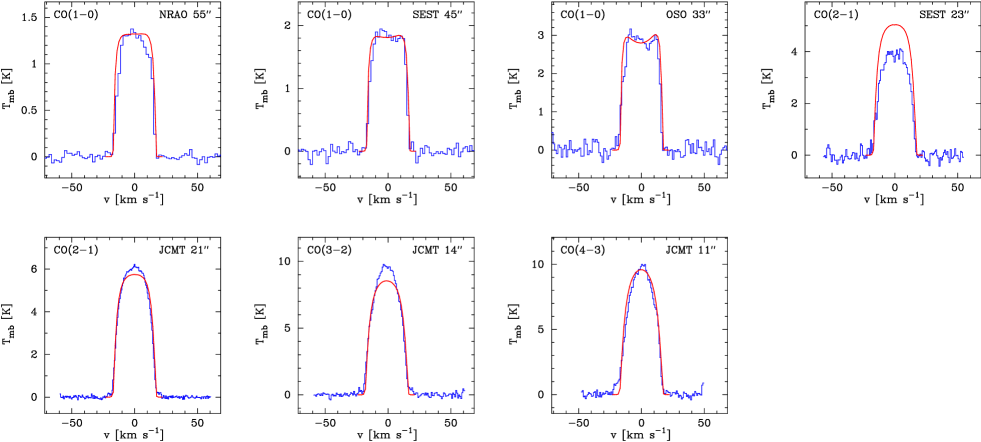
Figure 3: Best fit model (full line) for RW LMi overlayed on observations (histogram). The CO transition, telescope used, and the beamsize, are given for each of the observations.

5 Results and discussion

In this section the constraints on the CSE characteristics, including the mass loss rate history, obtained from the radiative transfer analysis of the CO line emission and the dust emission are presented. In addition, the influence of the dust component on the excitation of CO is investigated.

5.1 Excitation analysis of CO

FIR CO line emission was detected by ISO towards the high mass loss rate carbon stars CW Leo, RW LMi, and IRAS 15194-5115, and we start with the analysis of these objects. The results of the radiative transfer modelling, varying $\dot{M}$ and the $h$-parameter, are presented in Fig. 2 in the form of $\chi^{2}$-maps with various levels of confidence indicated. There are three $\chi^{2}$-maps per object, showing the constraints put by the radio and FIR observations individually and that of the combined full data set. For low to intermediate mass loss rate objects it is possible to constrain $\dot{M}$ and $h$ simultaneously from radio observations, provided that multi-transition observations are available (Schöier & Olofsson 2001). However, it is evident that for high mass loss rate objects, i.e., stars with $\dot{M}$$\gtrsim$10^-5 M_☉ yr^-1, only the integrated intensities from the observed millimeter lines are not enough to put good constraints on the mass loss rate. This is a consequence of the self-consistent treatment of the CO line cooling, where an increase of the mass loss rate leads to more cooling which compensates for the increase in molecular density [see discussion in Schöier & Olofsson (2001) for details].

By combining the radio data with the additional constraints put by the FIR ISO data it is possible to constrain both $\dot{M}$ and $h$ also for the more extreme carbon stars. Using the additional information on the excitation conditions contained in the shape of the, spectrally resolved, CO radio lines it is occasionally possible to further constrain the parameter space. For example, in the case of CW Leo models below $\sim$10^-5 M_☉ yr^-1 have $J$$=$1$\rightarrow$0 line-shapes that are double-peaked indicating optically thin resolved emission. This is, however, not observed. Moreover, models with mass loss rates in excess of $\sim$5$\times$10^-5 M_☉ yr^-1 are too optically thick and produce parabolic line shapes that are too centrally peaked when compared with the $J$$=$1$\rightarrow$0 line-shapes. Estimates of the mass loss rate and the $h$-parameter obtained from the full set of data are presented in Table 5. The FIR CO line fluxes obtained from the best fit models are presented in Tables 2$-$4. In Fig. 3 the line intensities obtained from the best fit model for RW LMi are overlayed on observations. Similar plots are presented for IRAS 15194-5115 in Ryde et al. (1999) and for CW Leo (radio data only) in Schöier & Olofsson (2001).

Table 3: Observed and modelled CO FIR rotational lines towards RW LMi.

$\lambda_{\mathrm{obs}}$	$F_{\mathrm{obs}}$	Transition	$\lambda_{\mathrm{vac}}$	$F_{\mathrm{mod}}$a
[$\mu$m]	[W cm-2]		[$\mu$m]	[W cm-2]
185.93	4.1$\times$10-20	CO(14-13)	185.999	4.0$\times$10-20
173.62	6.5$\times$10-20	CO(15-14)	162.811	4.5$\times$10-20
162.83	4.7$\times$10-20	CO(16-15)	162.811	4.5$\times$10-20
153.24	6.6$\times$10-20	CO(17-16)	153.267	4.7$\times$10-20
144.70	4.4$\times$10-20	CO(18-17)	144.784	4.9$\times$10-20
130.32	6.1$\times$10-20	CO(20-19)	130.369	5.2$\times$10-20
124.32	6.2$\times$10-20	CO(21-20)	124.193	5.3$\times$10-20
118.61	5.5$\times$10-20	CO(22-21)	118.581	5.5$\times$10-20
108.85	5.1$\times$10-20	CO(24-23)	108.763	5.6$\times$10-20
104.49	5.0$\times$10-20	CO(25-24)	104.445	5.7$\times$10-20
96.89	4.6$\times$10-20	CO(27-26)	96.773	5.8$\times$10-20
93.52	5.9$\times$10-20	CO(28-27)	93.349	5.8$\times$10-20
90.14	6.1$\times$10-20	CO(29-28)	90.163	5.8$\times$10-20

^a A mass loss rate of 5.0$\times$10^-6M_☉yr^-1 and a $h$-parameter of 2.3 was used in the modelling.

The quality of the best fit models can be judged from their reduced $\chi^{2}$ obtained from

$$\chi^{2}_{\mathrm{red}}=\frac{\chi^{2}_{\mathrm{min}}}{N-p},$$ (7)

where $p$ is the number of adjustable parameters, in this case two. In all cases the best fit model has $\chi^{2}_{\mathrm{red}}$$\sim$1, indicating a good fit.

Table 4: Observed and modelled CO FIR rotational lines towards IRAS 15194-5115.

$\lambda_{\mathrm{obs}}$	$F_{\mathrm{obs}}$	Transition	$\lambda_{\mathrm{vac}}$	$F_{\mathrm{mod}}$a
[$\mu$m]	[W cm-2]		[$\mu$m]	[W cm-2]
185.99	3.0$\times$10-20	CO(14-13)	185.999	2.6$\times$10-20
173.66	3.8$\times$10-20	CO(15-14)	162.811	2.8$\times$10-20
162.85	4.2$\times$10-20	CO(16-15)	153.267	3.0$\times$10-20
153.38	4.0$\times$10-20	CO(17-16)	144.784	3.1$\times$10-20
144.80	3.8$\times$10-20	CO(18-17)	137.196	3.3$\times$10-20
137.12	3.5$\times$10-20	CO(19-18)	130.369	3.4$\times$10-20
124.10	2.8$\times$10-20	CO(21-20)	118.581	3.7$\times$10-20

^a A mass loss rate of 1.2$\times$10^-5M_☉yr^-1 and a $h$-parameter of 2.8 was used in the modelling.

Figure 4: $\chi^{2}$-maps showing the sensitivity of the dust radiative transfer model, using the spectral energy distribution as constraint, to the dust opacity at 10 $\mu$m ($\tau_{10}$) and the dust condensation temperature ($T_{\mathrm{c}}$). Contours are drawn at the 1, 2 and 3$\sigma$ levels. The number of observational constraints, $N$, are also given. The quality of the best fit models are very good as determined from their reduced chi-squared statistics, $\chi^{2}_{\mathrm{red}}$ $\sim$1.

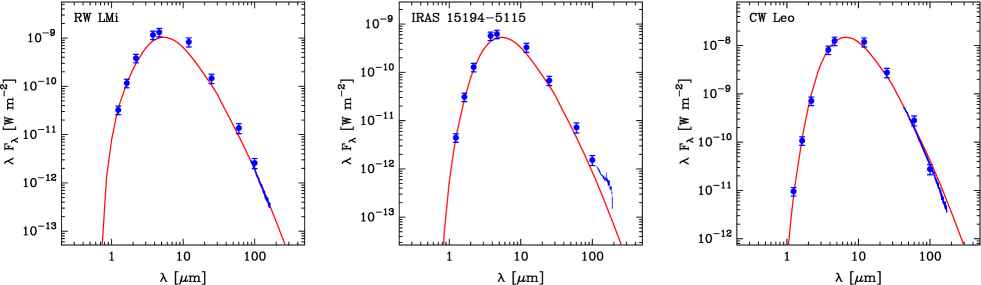
Figure 5: Spectral energy distributions of RW LMi, IRAS 15194-5115, and CW Leo obtained from the best fit dust radiative transfer model (full line). Filled circles with error bars indicate observed fluxes used in the $\chi^{2}$-analysis. Also shown is the ISO FIR spectrum between $\sim$100$-$200 $\mu$m. The latter was not used to constrain the dust radiative transfer modelling.

A detailed discussion on the excitation of CO, and also the sensitivity of the results of our standard model to variations of many of the input parameters, can be found in Ryde et al. (1999), Schöier & Olofsson (2000), and Schöier & Olofsson (2001).

5.2 Dust emission

The dust analysis is only performed for the high mass loss rate carbon stars CW Leo, IRAS 15194-5115, and RW LMi where ISO detected CO line emission. The observational constraints, in the form of SEDs covering the wavelength range $\sim$1$-$100 $\mu$m, consist of IRAS fluxes and $JHKLM$-photometry and are presented in Fig. 5 with the result from the best fit dust models superimposed. The near-infrared data taken at maximum light were obtained from Le Bertre (1992) for CW Leo and IRAS 15194-5115 and from Taranova & Shenavrin (1999) for RW LMi. The fits to the observed SEDs are very good and show no signs of any drastic modulation of the mass loss rate. In comparison, the presently known detached shell sources show a distinct excess in their 60 $\mu$m flux due to a brief, but intense, period of dramatically enhanced mass loss (Olofsson et al. 1996, 2000; Lindqvist et al. 1999; Schöier & Olofsson 2001)

The dust optical depth, Eq. 6, can be expressed in terms of the gas mass loss rate by using the gas-to-dust mass ratio, $\Psi$,

$$\tau_{\lambda}=\frac{\kappa_{\lambda}\Psi\dot{M}}{4\pi r_{\mathrm{i}}v_{\mathrm{d}}},$$ (8)

assuming $r_{\mathrm{e}}$$\gg$$r_{\mathrm{i}}$. The optical depth for the best fit dust model can be translated into a mass loss rate estimate using the combination of dust parameters as expressed by the $h$-parameter derived from the gas modelling and the expression for the drift velocity in Eq. 3. The mass loss rates obtained in this fashion are presented in Table 5 and they are all in excellent agreement with those presented in Ivezić & Elitzur (1995) and Groenewegen et al. (1998). The mass loss rates derived from the dust modelling agree well with those estimated from the CO line emission, putting further constraints on the mass loss rate history.

In the derivation of the mass loss rates for these extreme carbon stars a constant value of 0.03 was used for the flux averaged momentum transfer efficiency $Q$. In a more detailed modelling of the wind dynamics $v_{\mathrm{e}}$, $v_{\mathrm{d}}$, and $Q$ will have radial dependences (e.g., Habing et al. 1994; Elitzur & Ivezić 2001). However, they reach their terminal values close to the star, and since no direct observational information is available from this complex region any radial dependence is neglected in the present analysis. The terminal value of Q will depend on the amount of dust present and its properties. The fact that the SEDs for the high mass loss rate objects presented in Fig. 5 peak at roughly the same wavelength ($\sim$5 $\mu$m), indicates that their terminal values of Q are similar. The drift velocity for these sources is $\sim$3 km s^-1, i.e., significantly lower than the terminal gas expansion velocity. In this case, the dominant heating term of the gas, Eq. 2, can be written

$$H_{\mathrm{dg}}\propto\frac{hv^{3}_{\mathrm{dr}}}{1+\frac{v_{\mathrm{dr}}}{v_{\mathrm{e}}}}\approx hv^{3}_{\mathrm{dr}}\propto hQ^{3/2}.$$ (9)

This means that the uncertainty in the product $hQ^{3/2}$ is the same as derived for $h$ when $Q$ is fixed, i.e., within $\sim$30%.

Table 5: Derived envelope parameters from the radiative transfer analysis.

	Gas modela				Dust modelb
	$\dot{M}$	$h$	$\chi^{2}_{\mathrm{red}}$		$\tau_{10}$	$T_{\mathrm{d}}(r_{\mathrm{i}})$	$r_{\mathrm{i}}$	$\dot{M}$	$\chi^{2}_{\mathrm{red}}$
Source	[M☉yr-1]					[K]	[cm]	[M☉yr-1]
RW LMi	5.0$\pm$1.0$\times$10-6	2.3$\pm$0.3	0.8		0.41$\pm$0.02	1050$\pm$100	2.2$\times$1014	3.5$\times$10-6	1.1
IRAS 15194-5115	1.2$\pm$0.5$\times$10-5	2.8$\pm$0.7	0.9		0.59$\pm$0.05	1200$\pm$150	1.5$\times$1014	3.5$\times$10-6	0.8
CW Leo	1.2$\pm$0.8$\times$10-5	1.8$\pm$0.5	1.4		0.95$\pm$0.07	1200$\pm$100	1.9$\times$1014	8.0$\times$10-6	1.9

^a The uncertainties are based on the 68% confidence level (1$\sigma$) from Fig. 2 for the combined data set (radio + ISO) and indicates the range of acceptable values for each adjustable parameter. However, note that the 68% confidence level has a non-rectangular form in the two dimensional parameter space.
^b The uncertainties are based on the 68% confidence level (1$\sigma$) from Fig. 4 and indicates the range of acceptable values for each adjustable parameter. However, note that the 68% confidence level has a non-rectangular form in the two dimensional parameter space. The uncertainty in the mass loss rate estimate from the dust radiative transfer is $\sim$30-40% and includes the uncertainty in the adopted $h$-parameter.

Figure 6: Dust temperature through the circumstellar envelope around RW LMi (solid line). For $r$$\gtrsim$10¹⁵ cm, $T_{\mathrm{d}}(r)$ is well described by a power-law $r^{-0.4}$. Also shown for comparison is the kinetic temperature of the gas, $T_{\mathrm{g}}(r)$, obtained from the best fit CO model.

5.3 Effect of dust emission on the excitation of CO

The effect of a dust emission component on the excitation of CO is tested for RW LMi. In Fig. 6 the derived dust and gas temperature structures are plotted. For $r$$\gtrsim$10¹⁵ cm, the dust temperature is well described by a power-law falling off as $r^{-0.4}$. Closer to the star optical depth effects come into play and $T_{\mathrm{d}}(r)$ decreases faster with distance. The dust and gas temperatures are clearly decoupled throughout the envelope.

In Fig. 7 the radial variations of the cooling terms are plotted. The cooling rate has been multiplied by a factor $\propto r^{4}$ for clarity (the heating due to dust-gas collisions is roughly proportional to $r^{-4}$). CO rotational line cooling is the dominant coolant in the region between $\sim$3$\times$10¹⁴ cm and $\sim$1$\times$10¹⁷ cm, where most of the emission from the observed CO transitions emanate. Closer to the star cooling due to H₂ line emission and heat exchange between dust and gas becomes important but very little emission from this part of the CSE contributes to the line emission observed.

The excitation analysis shows that only in the innermost parts of the envelope is the $v$$=$1 state significantly populated, and hence able to affect the ground-state populations, but this region is severely diluted in the observational beams, and the derived line intensities are therefore not notably affected. In conclusion, the addition of a dust emission component has only a minor effect on the derived FIR line intensities, and no effect on the radio line intensities. Kwan & Hill (1977) noted that dust emission have no effect on the excitation of the radio lines using the large-velocity-gradient method, a less detailed treatment than ours of the radiative transfer problem.

Figure 7: The cooling rates in the CSE around RW LMi derived from the best fit model. The full line represents adiabatic cooling; the dotted line H₂ line cooling; the dashed line the CO line cooling; and the dash-dotted line cooling due to heat exchange with the dust. The cooling rates have been multiplied by a factor $\propto$$r^{4}$ for clarity. Note that for $r$$\gtrsim$10¹⁵ cm $T_{\mathrm{d}}$$>$$T_{\mathrm{g}}$ and the dust will heat the gas. This extra heating is, however, insignificant compared to the heating provided by dust-gas collisions.

5.4 Mass loss rate modulations

It is found that the CO radio lines are formed mainly beyond 5$\times$10¹⁶ cm, corresponding to a time scale of $\ga$10³ yr, while the FIR lines are formed much closer to the star, within $\sim$2$\times$10¹⁵ cm, which corresponds to $\la$40 yr. Thus, the CO emission modelled here traces the mass loss history over the past several thousand years. The dust parameters, as represented by the $h$-parameter, are not likely to have significantly changed during such a relatively short period of time. This is further supported by the radiative transfer analysis of the dust emission.

From the shape of the $\chi^{2}$-maps in Fig. 2 it is clear that the FIR fluxes are degenerate, with respect to the mass loss rate and the $h$-parameter, to some degree making it hard to put good constraints on any possible mass loss rate modulations. An increase in the mass loss rate, and hence the CO density, can be compensated for by lowering the $h$-parameter and thus the temperature in the envelope producing more or less the same amount of flux. In the case of RW LMi mass loss rate modulations of a factor of $\sim$2 (1$\sigma$) to $\sim$5 (2$\sigma$) are possible. For CW Leo and IRAS 15194-5115, such constraints can not be obtained from the analysis of the CO emission alone.

The dust emission typically probe the same radial extent of the envelope as the CO emission. The quality of the model fits obtained in the analysis of the SEDs are encouraging (Sect. 5.3) and fully consistent with a scenario where the average mass loss rate has been constant over a large period of time. The good agreement between the mass loss rates derived from the dust and the gas modelling strengthen the conclusion that any long-term mass loss rate modulations over the past thousands of years are likely to have been less than a factor of $\sim$5 for these stars. We conclude, for all three sources, that the average mass loss rate over the last $\sim$100 years is not substantially different from that over the last few thousand years.

Table 6: Observed and modelled FIR fluxes for sample stars where only upper limits were obtained.

Source	$F_{\mathrm{obs}}$a	$F_{\mathrm{mod}}$b
	[W cm-2]	[W cm-2]
V384 Per	$<$2$\times$10-20	5.5$\times$10-21
Y CVn	$<$8$\times$10-21	2.3$\times$10-21
V Cyg	$<$4$\times$10-20	1.7$\times$10-20
S Cep	$<$3$\times$10-20	9.3$\times$10-21
AFGL 3068	$<$2$\times$10-20	1.4$\times$10-20
LP And	$<$3$\times$10-20	1.5$\times$10-20

^a Upper limit to the CO FIR line emission from observations.
^b Predicted ISO flux from the model in the CO($J$$=$21$\rightarrow$20) transition using the envelope parameters from Table 1.

5.5 Non detections

The CSE parameters presented in Table 1 are used to calculate the model fluxes in the CO($J$$=$21$\rightarrow$20) transition for the objects not detected by ISO. The predicted fluxes are given and compared with the upper limits obtained from the ISO observations in Table 6. The model fluxes and the observed upper limits are all consistent with the scenario of a constant mass loss rate, or, to be more precise, a mass loss rate which has not increased significantly over the last 10³ years. It is also clear that far too little ISO observing time was spent on each of these six stars.

6 Conclusions

The modelling of CO rotational line emission at millimetre and FIR wavelengths put constraints on the physical properties of a CSE. Since the available data probe the full radial extent of the CO envelope conclusions about temporal changes in the mass loss rate can be drawn. For the high mass loss rate objects we find that the FIR data, which probe the inner regions of the CSE, are consistent with the results obtained from the radio data. Under the assumptions of a constant mass loss rate the combined set of data better constrain the envelope parameters such as the mass loss rate and the kinetic temperature of the gas.

From the CO data alone, it is generally hard to put good constraints on any modulations of the mass loss rate. However, analysis of the dust emission put further constraints on the mass loss rate history, and allows conclusions about its temporal changes to be drawn. We find that any longer-term mass loss rate modulations are likely to have been smaller than a factor of $\sim$5 over the past $\la$10⁴ yr.

The role of dust in the excitation of CO has been investigated and found to be of only minor importance.