NH₃ in the Central 10 pc of the Galaxy. II. Determination of Opacity for Gas with Large Linewidths

Abstract

The 23 GHz emission lines from the NH₃ rotation inversion transitions are widely used to investigate the kinematics and physical conditions in dense molecular clouds. The line profile is composed of hyperfine components which can be used to calculate the opacity of the gas (Ho & Townes, 1983). For intrinsic linewidths of a few km s^-1, the 18 magnetic hyperfine components blend together to form a line profile composed of five quadrupole hyperfine lines. If the intrinsic linewidth exceeds one half of the separation of these quadrupole hyperfine components ($\sim 5-10$ km s^-1) these five lines blend together and the observed linewidths greatly overestimate the intrinsic linewidths. If uncorrected, these artificially broad linewidths will lead to artificially high opacities. We have observed this effect in our NH₃ data from the central 10 pc of the Galaxy where uncorrected NH₃(1,1) linewidths of $\sim 30$ km s^-1 exaggerate the intrinsic linewidths by more than a factor of two (Genzel & Townes, 1987). Models of the effect of blending on the line profile enable us to solve for the intrinsic linewidth and opacity of NH₃ using the observed linewidth and intensity of two NH₃ rotation inversion transitions. By using the observed linewidth instead of the entire line profile, our method may also be used to correct linewidths in historical data where detailed information on the shape of the line profile is no longer available. We present the result of the application of this method to our Galactic Center data. We successfully recover the intrinsic linewidth ($\langle\Delta\rm{v}_{int}\rangle\approx 15$ km s^-1) and opacity of the gas. Clouds close to the nucleus in projected distance as well as those that are being impacted by Sgr A East show the highest intrinsic linewidths. The cores of the “southern streamer” (Ho et al., 1991; Coil & Ho, 1999, 2000) and the “50 km s^-1” giant molecular cloud (GMC, Güsten, Walmsley, & Pauls (1981)) have the highest opacities.

1 Introduction

The metastable (J=K) rotation inversion transitions of NH₃ are effective tracers of dense molecular material ($\rm{N_{H}}\approx 10^{4}-10^{5}$ cm^-3) (Ho & Townes, 1983). The NH₃ rotation inversion transitions are most often used to trace dense cores of giant molecular clouds (GMCs), but they are also observed in the “streamers” near the Galactic Center (Ho et al., 1991; Coil & Ho, 1999, 2000; McGary et al., 2001) which will be our example data for this paper. With frequencies near 23 GHz (1.3 cm), these transitions are easily observable with radio telescopes such as the Very Large Array (VLA) with only minimal interference by the atmosphere. Compared to high frequency tracers such as the 3 mm transitions of HCN(J=1-0) and HCO⁺(J=1-0) which often have $\tau>1$, these NH₃ transitions tend to be more optically thin, even in the case of low temperatures. As a result, spectra of NH₃ rotation inversion transitions are usually free of self-absorption effects.

The NH₃ rotation inversion line is composed of 18 magnetic hyperfine lines which are grouped into five main features (a detailed description of the NH₃ rotation inversion transitions can be found in Townes & Schalow (1975) and Ho & Townes (1983)). The spacing of the magnetic hyperfine lines within each of the five components is too close to resolve except in cool and quiescent dense cores where the intrinsic linewidths of the gas can be less than 1 km s^-1. The effect of blending of the 18 magnetic hyperfine components on the observed linewidth is discussed in detail in Ho et al. (1977) and Barranco & Goodman (1998). For linewidths of a few km s^-1, the magnetic hyperfine components within each of the five features will blend together to form five electric quadrupole hyperfine components consisting of a main line and two symmetric pairs of satellite lines. In this paper, we focus on large intrinsic linewidths and therefore will only concern ourselves with this “five-peak” profile. These quadrupole satellite lines are located from 10 to 30 km s^-1 from the main line (see Table 1 for relative spacings and intensities). Comparison of the intensity of a satellite line to the main line enables a direct calculation of the opacity of the gas making the NH₃ rotation inversion transitions especially useful. The derived opacity can then be used to calculate $N_{H}$, masses, and also combined with line ratios of different transitions to determine the rotational temperature of the gas (Ho & Townes, 1983).

The small frequency separation of the five quadrupole hyperfine lines means that for large intrinsic linewidths, $\Delta\rm{v}_{int}$, the satellite and main hyperfine components will be blended into a single line. Figure 1 shows line profiles for NH₃(1,1) for a range of intrinsic linewidths for $\tau_{\rm{m}}\ll 1$. For $\Delta\rm{v}_{int}\gtrsim 5$ km s^-1 the five components are blended into a single profile and it becomes difficult to measure the relative intensities needed for opacity estimation. The situation is aggravated by the fact that an increase in opacity will result in an increase in the intensity of the satellite hyperfine lines relative to the main line and the blended profile will appear to broaden even more. As a result, an increase in either $\tau_{\rm{m}}$ or $\Delta\rm{v}_{int}$ will appear as an increase in the observed linewidth, $\Delta\rm{v}_{obs}$, and it is difficult to interpret the data. Exaggerated estimates of opacity as a result of mis-fitting intrinsically broad lines can greatly limit the physical parameters that can be determined from the data. For example, if NH₃(1,1) gas has $\Delta\rm{v}_{int}>5$ km s^-1, then an increase in linewidth may be mistaken as an increase in opacity. The overestimation of the opacity propagates into overestimations of the column density and ultimately the calculated mass of the gas. In the case of our Galactic Center data, the observed linewidths are high and the challenge is to determine the extent of the contribution from shocked material with large intrinsic linewidths as well as that from high opacity gas. Shocks are important for identifying the locations of possible interactions between the streamers of molecular material that surround the Galactic Center. A mistaken calculation of the mass of a cloud or incorrect identification of a shock could affect our general understanding of the environment in the central parsecs of the Galaxy. It is therefore obvious that we need an improved method to obtain independent estimates of the opacity and intrinsic linewidth of the gas.

In this paper, we present a method to disentangle the effects of large intrinsic linewidths and high opacities by comparing the observed linewidths and intensities of two NH₃ transitions. Because the exact shape of the line profile need not be known, this method can be easily applied to historical data where the line profiles are no longer available. Throughout the paper, we combine the theoretical discussion with a test case example using our NH₃(1,1), (2,2), and (3,3) data from the Galactic Center. In §2, we show the correlation between $\Delta\rm{v}_{obs}$ and $\tau_{\rm{m}}$ in our Galactic Center data when the two quantities are solved for in the traditional manner. Section 3.1 then presents a calculation of the dependence of $\Delta\rm{v}_{obs}$ on $\Delta\rm{v}_{int}$ for NH₃(1,1), (2,2), and (3,3) for the special case where $\tau_{\rm{m}}\ll 1$. This is followed by the incorporation of variations in opacity. The full method for simultaneously solving for the opacity and intrinsic linewidth is presented in §4. The paper concludes by presenting the maps of the best estimate of $\Delta\rm{v}_{int}$ and NH₃(1,1) opacity for our Galactic Center data. The map of intrinsic linewidths shows $\langle\Delta\rm{v}_{int}\rangle=15$ km s^-1 for NH₃(1,1) which is in agreement with observations of other tracers. In addition, the corrected opacities show that all except the most massive features in the map are optically thin. The opacity and intrinsic linewidths of the observed features are then discussed.

2 The Observed Correlation between $\Delta\rm{v}_{obs}$ and $\tau_{\rm{m}}$

Gas near the Galactic center has been observed to have intrinsic linewidths of 10–20 km s^-1, and therefore provides a good test of the effects of blending of hyperfine lines on the calculation of the opacity (Güsten & Downes, 1980; Armstrong & Barrett, 1985). We observed the central 10 pc of the Galaxy in NH₃(1,1), (2,2), and (3,3) in 1999 March (McGary et al., 2001). The data were taken at 23 GHz in the D-northC configuration of the Very Large Array (VLA) to provide the largest and most circular beam possible. A Gaussian taper was applied to the $uv$ data resulting in a synthesized beam of $15^{\prime\prime}\times 13^{\prime\prime}$, which is useful for detection of extended features in our maps. The data have a velocity coverage of $\pm 150$ km s^-1, which includes almost all detected motions at the Galactic Center, and a velocity resolution of 9.8 km s^-1. In addition, a five pointing mosaic ensures full spatial coverage of the region. We choose the rotation inversion transitions of NH₃ so that we can directly use the hyperfine lines to calculate the opacity of the gas. The opacity is then combined with line ratios to calculate the rotational temperature of features observed in the central 10 pc (Ho & Townes, 1983). Increased temperatures can be a sign of shocked gas which is important in determining if there are cloud-cloud collisions or shocks from the expanding supernova remnant, Sgr A East (Genzel et al., 1990; Ho et al., 1991; Serabyn, Lacy, & Achtermann, 1992; Zylka, 1999). Accurate measurements of the intrinsic linewidth of the gas are also important for locating shocked regions. The large photon flux from the nucleus may also heat gas, and features close to the Galactic Center should appear warmer. All of these quantities depend on accurate measurements of the opacity and intrinsic linewidth of the gas.

We initially solved for the opacity in the traditional manner by comparing the flux density of the main component to the average flux density of the two outermost hyperfine components ($\pm 19.3$ km s^-1 for NH₃(1,1)). By averaging these two lines, we increase the S/N by a factor of $\sqrt{2}$ and opacities are only calculated where this average hyperfine flux density is greater than $3/\sqrt{2}\sigma_{\rm{JK}}$ where $\sigma_{11}=0.009$ Jy Beam^-1, $\sigma_{22}=0.009$ Jy Beam^-1, and $\sigma_{33}=0.011$ Jy Beam^-1. From radiative transfer, the opacity is related to the observed flux density of the main and satellite hyperfine lines by

$$\frac{S(\nu)_{m}}{S(\nu)_{s}}=\frac{[\Delta T_{A}(\nu)]_{m}}{[\Delta T_{A}(\nu)]_{s}}=\frac{1-e^{-\tau(\nu)_{m}}}{1-e^{-a\tau(\nu)_{m}}}$$ (1)

where $S(\nu)_{m}$ and $S(\nu)_{s}$ refer to flux densities of the main and satellite lines, $[\Delta T_{A}(\nu)]_{m}$ and $[\Delta T_{A}(\nu)]_{s}$ are the respective antenna temperatures, $\tau(\nu)_{m}$ is the opacity of the main hyperfine component, and $a$ is the theoretical intensity of the satellite line compared to the main line for $\tau(\nu)\ll 1$. Note that this equation assumes equal beam filling factors and excitation temperatures for the two transitions. The theoretical relative intensities of the quadrupole satellite hyperfine lines for NH₃(1,1), (2,2), and (3,3) are listed in Table 1.

Meanwhile, an observed linewidth, $\Delta\rm{v}_{obs}$ (defined in this paper as the FWHM), is fit to every pixel in the map by fitting a Gaussian of the form

$$f(\rm{v})=A_{0}e^{\frac{-(\rm{v}-\rm{v}_{0})^{2}}{2\sigma_{obs}^{2}}}$$ (2)

where $\rm{v}_{0}$ is the peak velocity at each position and $\Delta\rm{v}_{obs}=2.35\sigma_{obs}$. Observed linewidths are only calculated for pixels where the peak flux in the channel corresponding to $\rm{v}_{0}$ is greater than $3\sigma_{\rm{JK}}$. The calculated observed linewidths are also required to be less than 100 km s^-1. The NH₃(1,1) data give $\langle\Delta\rm{v}_{obs}\rangle=30$ km s^-1 which is approximately a factor of two larger than what is observed in other tracers (Güsten & Downes, 1980; Armstrong & Barrett, 1985; Genzel & Townes, 1987). Linewidths calculated from the NH₃(3,3) data, however, have $\langle\Delta\rm{v}_{obs}\rangle=18$ km s^-1. For $\tau_{\rm{m}}\ll 1$, the NH₃(1,1) satellite hyperfine lines are a much larger fraction of the main line intensity (28 and 22%) than in the case of NH₃(3,3) ($\sim 3$%). In addition, the NH₃(1,1) quadrupole hyperfine lines have a much smaller velocity separation than the higher transitions (see Table 1). These two characteristics of NH₃(1,1) make it much more susceptible to corruption by blending of the quadrupole hyperfine lines at large intrinsic linewidths. The difference in the observed linewidths for the NH₃(1,1) and (3,3) data may thus be explained by the large intrinsic linewidths near the Galactic Center.

To test whether blending has affected the NH₃(1,1) data, we plot $\Delta\rm{v}_{obs}$ as a function of the main line opacity, $\tau_{\rm{m}}(1,1)$ for every pixel in our NH₃(1,1) map where $\Delta\rm{v}_{obs}<100$ km s^-1 and $\tau_{\rm{m}}(1,1)<5$ (see Figure 2$a$). The main line opacity has been calculated using Equation 1 and the relative intensities of the main and outer satellite hyperfine lines. The noise in one channel, $\sigma_{11}$, results in an estimated error of $\sim 0.1$ for $\tau_{\rm{m}}(1,1)$. The error in $\Delta\rm{v}_{obs}$ is 1–2 km s^-1(see §4.1). A strong correlation between the two quantities is observed. However, there are many pixels per $\sim 15^{\prime\prime}$ beam resulting in correlation between adjacent pixels. In Figure 2$b$, we average over the beam and sample once per beam resulting in independent pixels. The correlation coefficient between $\Delta\rm{v}_{obs}$ and $\tau_{\rm{m}}(1,1)$ is 0.69. Figure 3 shows the same parameters for NH₃(3,3) and the correlation coefficient between $\Delta\rm{v}_{obs}$ and $\tau_{\rm{m}}(3,3)$ is only 0.07. The fact that the correlation is weaker in NH₃(3,3) than (1,1) suggests that the correlation between $\Delta\rm{v}_{obs}$ and $\tau_{\rm{m}}(1,1)$ is not real, but is an artifact of blending of the hyperfine components. It is interesting to note that there are no points with $\tau_{\rm{m}}(3,3)<1.0$ in this figure. This effect is explained by the minimum flux cutoff of $3\sigma_{33}$ (0.03 Jy beam^-1) required for the average outer satellite hyperfine line. Because the satellite hyperfine lines are intrinsically weaker in NH₃(3,3) than in (1,1) (see Table 1), the (3,3) hyperfine lines are often below this noise cutoff resulting in an effective cutoff in the minimum $\tau_{\rm{m}}(3,3)$ to which we are sensitive.

3 Dependence of $\Delta\rm{v}_{obs}$ on $\Delta\rm{v}_{int}$ and $\tau_{\rm{m}}$

In order to develop a method to remove the effects of blending on $\Delta\rm{v}_{obs}$, we must model the dependence of the observed linewidth on both the intrinsic linewidth and the opacity of the gas. The opacity of the gas as a function of velocity is defined as

$$\tau(\rm{v})=\tau_{m}\phi(\rm{v},\sigma)$$ (3)

where $\tau_{\rm{m}}$ is the opacity at the center of the main line and $\phi(\rm{v},\sigma)$ is the normalized line profile for the rotation inversion transition. The quadrupole hyperfine components are modeled by five Gaussians with velocity spacings and relative intensities of the satellite hyperfine lines defined as in Table 1. The profile is written explicitly as

$$\phi(\rm{v},\sigma)= e^{-\rm{v}^{2}/2\sigma_{int}^{2}}$$ (4)

$$+ a_{\rm{in}}e^{-(\rm{v}-\Delta\rm{v}_{in})^{2}/2\sigma_{int}^{2}}+a_{\rm{in}}e^{-(\rm{v}+\Delta\rm{v}_{in})^{2}/2\sigma_{int}^{2}}$$

$$+ a_{\rm{out}}e^{-(\rm{v}-\Delta\rm{v}_{out})^{2}/2\sigma_{int}^{2}}+a_{\rm{out}}e^{-(\rm{v}+\Delta\rm{v}_{out})^{2}/2\sigma_{int}^{2}}$$

where $\sigma_{\rm{int}}=\Delta\rm{v}_{int}/2.35$ is the standard deviation of the line profile, $\Delta\rm{v}_{in}$ and $\Delta\rm{v}_{out}$ are the offsets of the inner and outer satellite hyperfine lines (in km s^-1) respectively, and $a_{\rm{in}}$ and $a_{\rm{out}}$ are the intensities of the inner and outer satellite hyperfine lines assuming an intensity of 1.0 for the main line (see Table 1). The intensity of the line is given by

$$\rm{I}(\rm{v},\sigma,\tau_{\rm{m}})=(T_{ex}-T_{b})[1-e^{-\tau_{m}\phi(\rm{v},\sigma)}]~{}.$$ (5)

Throughout the paper, when the opacity is referred to in the general case, we use $\tau_{\rm{m}}$. For a specific (J,K) transition of NH₃, the main line opacity is written as $\tau_{\rm{m}}$(J,K). It is this opacity of the main line, $\tau_{m}$, that is reported in most observational papers and in keeping with this convention, the opacities derived in this paper all refer to $\tau_{m}$.

3.1 Dependence of $\Delta\rm{v}_{obs}$ on $\Delta\rm{v}_{int}$ for $\tau_{\rm{m}}\ll 1$

We begin by calculating the line profile as a function of $\Delta\rm{v}_{int}$ in the special case where $\tau_{\rm{m}}\ll 1$. We need not be concerned with the observed value of $\rm{I}(\rm{v},\sigma,\tau_{\rm{m}})$ because the FWHM and relative intensity of the main and satellite hyperfine lines are independent of the absolute amplitude of the line. Therefore, Equation 5 reduces to $\rm{I}(\rm{v},\sigma,\tau_{\rm{m}})\propto\phi(\rm{v},\sigma)$ for $\tau_{\rm{m}}\ll 1$. Figure 1 compares the line profiles of NH₃(1,1) for $\tau_{\rm{m}}\ll 1$ for a range of intrinsic linewidths. For $\Delta\rm{v}_{int}\gtrsim 5$ km s^-1, the main and satellite components of NH₃(1,1) blend into a single line profile and fitting a Gaussian profile to the main component will overestimate the intrinsic linewidth of the gas.

In order to determine $\Delta\rm{v}_{obs}$ as a function of $\Delta\rm{v}_{int}$ for NH₃(1,1), (2,2), and (3,3), normalized line profiles as a function of $\Delta\rm{v}_{int}$ and v are generated for the case where $\tau_{\rm{m}}\ll 1$. For each normalized line profile, a Gaussian is fit to the main component to determine the resulting observed linewidth. By modeling the effect of $\Delta\rm{v}_{int}$ and $\tau_{\rm{m}}$ on the observed linewidth, the method for recovering the intrinsic linewidth can be applied to any historical data where the entire line profile may no longer be available. Figure 4$a$ shows $\Delta\rm{v}_{obs}$ as a function of $\Delta\rm{v}_{int}$ for NH₃ (1,1), (2,2), and (3,3) assuming $\tau_{\rm{m}}\ll 1$. For $\Delta\rm{v}_{int}\lesssim 5$ km s^-1, no blending occurs and all three transitions have $\Delta\rm{v}_{obs}\approx\Delta\rm{v}_{int}$. Note that we are not concerned with the case of dark cores where intrinsic linewidths of only a few km s^-1 cause the closely separated 18 magnetic hyperfine lines to blend, which is discussed in detail in Ho et al. (1977) and Barranco & Goodman (1998).

For intrinsic linewidths greater than 5 km s^-1, the satellite hyperfine lines of NH₃(1,1) blend with the main line and $\Delta\rm{v}_{obs}(1,1)$ will greatly exaggerate $\Delta\rm{v}_{int}$ for $\Delta\rm{v}_{int}\gtrsim 5$ km s^-1, independent of opacity and velocity resolution. NH₃(2,2) and (3,3) give a much better estimation of the intrinsic linewidth for $\tau_{\rm{m}}\ll 1$ because the satellite hyperfine lines are relatively weaker compared to the main lines and are also located further from the main line than in the case of NH₃(1,1). In our Galactic Center data, we find $\langle\Delta\rm{v}_{obs}\rangle=30$ km s^-1 for NH₃(1,1) and $\langle\Delta\rm{v}_{obs}\rangle=18$ km s^-1 for NH₃(3,3). These results can be fit almost exactly by $\Delta\rm{v}_{int}=17$ km s^-1 in Figure 4$a$.

Figure 4$b$ plots $\Delta\rm{v}_{obs}/\Delta\rm{v}_{int}$ for intrinsic linewidths up to 60 km s^-1. For each transition, there exists a velocity, $\rm{v_{crit}}$, above which the exaggeration of $\Delta\rm{v}_{int}$ by $\Delta\rm{v}_{obs}$ decreases. As the intrinsic linewidths approach $\rm{v_{crit}}$, the line profile is broadening as the satellite hyperfine lines blend with the main line. However, once the intrinsic linewidth of the gas is greater than the maximum separation of the hyperfine lines, the effect of the satellite hyperfine lines on $\Delta\rm{v}_{obs}$ becomes less important and $\Delta\rm{v}_{obs}$ asymptotically approaches $\Delta\rm{v}_{int}$. The critical velocities for NH₃(1,1), (2,2), and (3,3) are 8, 20, and 27 km s^-1, respectively. For the Galactic Center where $\Delta\rm{v}_{int}\approx 15$ km s^-1, NH₃(1,1) gives by far the worst overestimation of $\Delta\rm{v}_{int}$. However, for $\Delta\rm{v}_{int}\lower 2.15277pt\hbox{$\;\buildrel>\over{\sim}\;$}50$ km s^-1, NH₃(2,2) is equally as bad as NH₃(1,1). For the remainder of this paper, we focus on $\Delta\rm{v}_{int}\leq 30$ km s^-1, as expected at the Galactic Center.

3.2 Observed line profiles as a function of $\Delta\rm{v}_{int}$ and $\tau$

In this section, we calculate line profiles for the case where the opacity is large enough that the intensity of the satellite hyperfine lines becomes important. In the case of the blended profile, an increase in opacity will appear as an increase in the observed linewidth of the profile. Figures 1 and 5 can be used to compare the effects of changes in either $\Delta\rm{v}_{int}$ or $\tau_{m}$ while the other parameter is held constant. As seen in Figure 1, an increase in $\Delta\rm{v}_{int}$ for constant opacity results in broadening of the line profile until the five quadrupole hyperfine lines blend together. Figures 5$a$ and 5$b$ show the effect of varying $\tau_{m}$ when $\Delta\rm{v}_{int}=3$ and 15 km s^-1 for NH₃(1,1). In Figure 5$a$, $\Delta\rm{v}_{int}<5$ km s^-1 so the profiles are not blended. As a result, an increase in $\tau_{m}$ only results in an increase in the relative intensities of the satellite lines with respect to the main line. In Figure 5$b$, however, the blended profile appears to broaden dramatically as the opacity is increased.

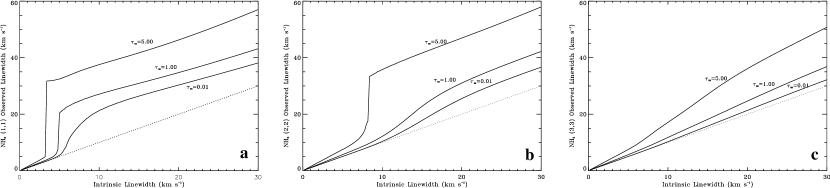
Figure 6: $\Delta\rm{v}_{obs}$ as a function of $\Delta\rm{v}_{int}$ for $\tau_{\rm{m}}=0.01,1.0,5.0$ for $a)$ NH₃(1,1), $b)$ NH₃(2,2) and $c)$ NH₃(3,3). The dashed line shows $\Delta\rm{v}_{obs}=\Delta\rm{v}_{int}$. For large $\tau_{\rm{m}}$, a discontinuity develops at $\sim 3$ km s^-1 for NH₃(1,1) and $\sim 8$ km s^-1 for NH₃(2,2) where blending of hyperfine lines with comparable intensities suddenly results in a very broad line profile.

Using the definition of the line profile in Equation 5, an array of line profiles is generated for a range of opacities and intrinsic linewidths. If the data have good velocity resolution with many channels across the profile, then the intrinsic linewidth and $\tau_{\rm{m}}$ of any NH₃ rotation inversion transition may be solved for without any additional information from other tracers. In this case, a least squares minimization routine can be used to search this array to find the $\Delta\rm{v}_{int}$ and $\tau_{\rm{m}}$ that give the best fit to the observed line profile. In the case where multiple transitions of NH₃ are observed, similar results may be easily obtained by comparing only the observed linewidths and intensities of the lines. For each line profile in the generated data, the main line is fit with a Gaussian to estimate the expected value for $\Delta\rm{v}_{obs}$. Figure 6 shows the dependence of $\Delta\rm{v}_{obs}$ on $\Delta\rm{v}_{int}$ and $\tau_{\rm{m}}$ for the simulated NH₃ (1,1), (2,2), and (3,3) data. For small intrinsic linewidths, the hyperfine components are well-separated and $\Delta\rm{v}_{obs}\approx\Delta\rm{v}_{int}$, independent of $\tau_{\rm{m}}$. A discontinuity develops near 5 km s^-1 for NH₃ (1,1) and 8 km s^-1 for NH₃(2,2) in the optically thick cases resulting from the blending of main and satellite hyperfine components with comparable intensities (see the line profile for $\tau_{\rm{m}}(1,1)=5.0$ in Figure 5$a$). NH₃(3,3) does not show this effect in our models because the satellite hyperfine lines are $<20\%$ of the intensity of the main component even in the case where $\tau_{\rm{m}}(3,3)=5.0$. Using Figure 6$a$, we find that for an average intrinsic linewidth at the Galactic Center data of 17 km s^-1 as in §3.1, the average observed linewidth of 30 km s^-1 in our data indicates that $0.01<\tau_{\rm{m}}(1,1)<1.0$.

4 Method to Simultaneously Determine $\Delta\rm{v}_{int}$, $\tau_{\rm{m}}(1,1)$, and $\tau_{\rm{m}}(3,3)$

In this section, we outline the detailed steps of our method for recovering the intrinsic linewidths and opacities of gas with large linewidths using our Galactic Center data as an example. We use NH₃ (1,1) and (3,3) because they are the brightest tracers in our data and thus have the most points for which $\Delta\rm{v}_{obs}$ can be calculated for both transitions. There is much NH₃(1,1) emission because it traces the lowest energy of the rotation inversion transitions (23.4 K above ground) (Ho & Townes, 1983). The NH₃(3,3) image is bright, however, due to a quantum degeneracy in the ‘ortho’ ($J=3\rm{n}$) form of NH₃ which increases its intensity by a factor of two (Ho & Townes, 1983). In addition, high temperatures near the Galactic Center make this transition well-populated.

Two assumptions must hold for the method to be valid. First, it is assumed that the two transitions have the same intrinsic linewidth. Our NH₃(1,1) and (3,3) velocity integrated maps display a very high degree of correspondence and it seems valid to postulate that the two transitions trace the same material and therefore should have the same intrinsic linewidth. In addition, it is necessary to assume that the opacity does not exceed a particular value, $\tau_{max}$, in either transition. This maximum opacity is used to limit the size of the parameter space which must be searched. In the case below, we have assumed $\tau_{max}=5$ for both NH₃(1,1) and (3,3). As seen in §5, almost all points in our dataset have final opacities less than 1.0, which is well below $\tau_{max}$.

The following four steps can be used to recover the intrinsic linewidth and opacity of NH₃ rotation inversion transitions when observed linewidths and intensities of two transitions are known.

(1) A Gaussian profile is fit to the upper transition, to obtain $\Delta\rm{v}_{obs}$. This upper transition is chosen because it will be less affected by blending and will give the best initial estimate of $\Delta\rm{v}_{int}$ (see Figure 4$b$). Using the NH₃(3,3) observed linewidth, $\Delta\rm{v}_{obs}(3,3)$, the relation between $\Delta\rm{v}_{obs}$ and $\Delta\rm{v}_{int}$ can be used to solve for a range of valid $\Delta\rm{v}_{int}$ corresponding to the case where $0<\tau_{\rm{m}}(3,3)<\tau_{max}$ (see Figure 6$c$). The range of valid intrinsic linewidths is denoted here as

$$\Delta\rm{v}_{int,low}<\Delta\rm{v}_{int}<\Delta\rm{v}_{int,high}~{}.$$ (6)

For example, Figure 6$c$ shows that if $\Delta\rm{v}_{obs}(3,3)=15$ km s^-1 then $9$km s^-1$\lesssim\Delta\rm{v}_{int}\lesssim 14$km s^-1 for $0\leq\tau_{\rm{m}}(3,3)\leq 5$.

(2) With a range of valid intrinsic linewidths, the NH₃(1,1) observed linewidth, $\Delta\rm{v}_{obs}(1,1)$, is used to find the range of acceptable NH₃(1,1) opacities. Each curve in Figure 7 corresponds to a different intrinsic linewidth. Therefore Step 1 enables the determination of a range of valid curves where $\Delta\rm{v}_{int,low}<\Delta\rm{v}_{int}<\Delta\rm{v}_{int,high}$. There is only a limited range of $\tau_{\rm{m}}(1,1)$ where the NH₃(1,1) observed linewidth lies between the minimum and maximum curves in Figure 7. In this way, $\Delta\rm{v}_{obs}(1,1)$ is combined with the range of intrinsic linewidths from Step 1 to calculate a valid range for $\tau_{\rm{m}}(1,1)$ such that

$$\tau_{\rm{m}}(1,1)_{\rm{low}}<\tau_{\rm{m}}(1,1)<\tau_{\rm{m}}(1,1)_{\rm{high}}~{}.$$ (7)

In the example discussed above, we know $9$km s^-1$\lesssim\Delta\rm{v}_{int}\lesssim 14$km s^-1. Now, if $\Delta\rm{v}_{obs}(1,1)=30$ km s^-1 then we can use Figure 7 to determine that $\tau_{\rm{m}}(1,1)$ must lie between 0.9 and 1.9.

(3) The NH₃(3,3) opacity can be calculated from the NH₃(1,1) opacity and the ratio of the brightness of the main lines of NH₃(3,3) to (1,1) using

$$\tau_{\rm{m}}(J,K)=-\ln[1-\frac{[\Delta T_{A}(\nu)]_{m}(J,K)}{[\Delta T_{A}(\nu)]_{m}(1,1)}(1-e^{-\tau_{\rm{m}}(1,1)})]~{}.$$ (8)

As stated in §2, this equation assumes equal beam filling factors and excitation temperatures for NH₃(1,1) and (3,3). Given the similarity of the velocity integrated maps for these two transitions (see McGary et al. (2001)), the assumption of equal beam filling factors is reasonable. In addition, the densities of $10^{4}-10^{5}$ cm^-3 in these clouds should result in thermalization that will tend to make the excitation temperatures of NH₃(1,1) and (3,3) equal. With these assumptions, a range of acceptable $\tau_{\rm{m}}(3,3)$ can be directly calculated using Equation 8 and the range of $\tau_{\rm{m}}(1,1)$ found in Step 2 such that

$$\tau_{\rm{m}}(3,3)_{\rm{low}}<\tau_{\rm{m}}(3,3)<\tau_{\rm{m}}(3,3)_{\rm{high}}~{}.$$ (9)

These new limits on $\tau_{\rm{m}}(3,3)$ provide a tighter constraint than our initial assumption that $0<\tau_{\rm{m}}(3,3)<\tau_{max}$.

(4) With a smaller range for $\tau_{\rm{m}}(3,3)$, we can return to Step $1$ and determine a tighter constraint for $\Delta\rm{v}_{int}$. It follows that this process can be repeated until it converges to a solution for $\Delta\rm{v}_{int}$, $\tau_{\rm{m}}(3,3)$, and $\tau_{\rm{m}}(1,1)$ within some predefined tolerance. In our data, we find that the solutions will converge in less than five iterations for a tolerance of 0.4 for $\tau_{\rm{m}}(1,1)$. The fast conversion of this method makes it especially useful for datasets with many pixels.

4.1 Estimated Errors

To estimate the error in $\Delta\rm{v}_{int}$ and $\tau_{\rm{m}}$, we first estimate the error in the fit of $\Delta\rm{v}_{obs}$ to a noisy line profile. Starting with the theoretical line profile, $\rm{I}(\rm{v},\sigma,\tau_{\rm{m}})$, noise is added at the 10% level and the observed linewidth, $\Delta\rm{v}_{obs}^{\prime}$, is measured. This observed linewidth is compared to the expected FWHM, $\Delta\rm{v}_{obs}$, found by fitting a Gaussian to the noiseless profile. The process is repeated until the spread in the differences between $\Delta\rm{v}_{obs}^{\prime}$ and $\Delta\rm{v}_{obs}$ can be used to estimate the error in observed linewidth. We first model the errors in NH₃(1,1) in the case where the channel width is much less than the separation of the hyperfine components. The largest errors (up to 3 km s^-1) occur for $\Delta\rm{v}_{int}\approx 5$ km s^-1 and $0.5<\tau_{\rm{m}}(1,1)<1.0$. In this case, the five hyperfine components are partially blended, making it difficult to properly estimate a linewidth for the main line. Elsewhere, the expected error in $\Delta\rm{v}_{obs}$ is less than 0.5 km s^-1. For $\Delta\rm{v}_{int}=15$ km s^-1, the error in the observed linewidth is 0.3 km s^-1 for a spectrum with $S/N=10$. For NH₃(3,3), the hyperfine components have a much smaller effect and the error in the fit to $\Delta\rm{v}_{obs}(3,3)$ is never greater than 0.5 km s^-1, independent of $\Delta\rm{v}_{int}$ and $\tau_{\rm{m}}(3,3)$.

For the Galactic center data discussed below, the channel width of 9.8 km s^-1 is close to the velocity separation of the hyperfine components and dominates the error for $\Delta\rm{v}_{int}<5$ km s^-1. However, our observations were planed with the knowledge that intrinsic linewidths at the Galactic center range between 10 and 20 km s^-1. For $\Delta\rm{v}_{int}\lower 2.15277pt\hbox{$\;\buildrel>\over{\sim}\;$}5$ km s^-1, the fit to $\Delta\rm{v}_{obs}$ is reasonable and the error ranges between 1 and 2 km s^-1 with a slight dependence on $\tau_{\rm{m}}(1,1)$ and $\Delta\rm{v}_{int}$. Assuming $\Delta\rm{v}_{int}=15$ km s^-1 for the Galactic Center, the $1\sigma$ error in the fit to $\Delta\rm{v}_{obs}(1,1)$ and $\Delta\rm{v}_{obs}(3,3)$ is 2 km s^-1and 1 km s^-1, respectively.

Simulations of the error in $\Delta\rm{v}_{int}$ and $\tau_{\rm{m}}(1,1)$ were made using an error of 2 km s^-1 for $\Delta\rm{v}_{obs}(1,1)$ and $\Delta\rm{v}_{obs}(3,3)$ and an error of 0.01 Jy beam^-1 for the amplitude of the NH₃(1,1) and (3,3) main lines. We find a typical error of 0.4 for $\tau_{\rm{m}}(1,1)$ and 4 km s^-1 for $\Delta\rm{v}_{int}$ with the caveat that the opacities and linewidths cannot be negative. In both cases, errors show a slight increase towards larger values of $\Delta\rm{v}_{int}$ and $\tau_{\rm{m}}(1,1)$. This results from the fact that the slope in Figures 6 and 7 becomes more shallow for large values of $\Delta\rm{v}_{int}$ and $\tau_{\rm{m}}(1,1)$.

5 Results for Galactic Center Data

We have applied the method above to our NH₃(1,1) and (3,3) Galactic Center data for all pixels with calculated linewidths less than 100 km s^-1. Each pixel was calculated individually and then the resulting map was smoothed with an eight pixel median filter to match the resolution intrinsic to our data. Because pixels for which no value can be determined are set to zero, a convolution by the beam would result in a halo of low values around all features in the map. As a result, every cloud would appear to be optically thin and have low intrinsic linewidths at the edge which could be misleading. The median filter will not produce this halo and is therefore better suited to be used in smoothing the data.

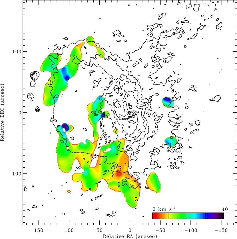
Figure 8: Best estimate of $\Delta\rm{v}_{int}$ in color overlaid on an image of 6 cm continuum emission in contours (Yusef-Zadeh & Morris, 1987). Contours are 0.001, 0.01, 0.02, 0.04, 0.08, 0.16, 0.32, 0.64, and 1.28 Jy beam^-1. The linewidth map has been smoothed with an eight pixel median filter (see §5). The continuum image shows the location of the expanding shell, Sgr A East, the mini-spiral, and Sgr A*. Typical intrinsic linewidths are 15 km s^-1. The largest $\Delta\rm{v}_{int}$ appear to be located near the nucleus or on the edge of Sgr A East.

Figure 8 shows the intrinsic linewidth of NH₃ in the central 10 pc of the Galaxy. The linewidths are in color while a 6 cm continuum emission image (Yusef-Zadeh & Morris, 1987) is overlaid in contours. The continuum map shows the outer edge of the expanding SNR, Sgr A East, as well as the ionized arms of the mini-spiral (Sgr A West). Emission associated with the $2.6\times 10^{6}$ M_⊙ supermassive black hole (Eckart & Genzel, 1997; Ghez et al., 1998), known as Sgr A*, is seen as the point source at the center of the map. Previous NH₃(1,1) observations of the Galactic Center find $\langle\Delta\rm{v}_{obs}(1,1)\rangle\sim 30$ km s^-1 for the region (Coil & Ho, 1999, 2000), similar to our original results. However, other molecular tracers including NH₃(3,3) show significantly smaller linewidths (Güsten & Downes, 1980; Armstrong & Barrett, 1985). Although the large linewidths in NH₃ (1,1) are attributed to the nearby hyperfine components, no previous attempt was made to recover the values of the intrinsic linewidths and subsequent calculations of the opacity did not take $\Delta\rm{v}_{int}$ into account. In Figure 8, we have applied our new method, and the average value of NH₃(1,1) intrinsic linewidth is $\sim 15$ km s^-1, which is in agreement with that of NH₃(3,3) and results from other tracers. Therefore, we find NH₃(1,1) has intrinsic linewidths between 10 and 20 km s^-1 in the central 10 pc of the Galaxy.

At first glance, the NH₃(1,1) linewidth appears similar throughout the map. However, there are many details of interest which merit discussion. Readers are referred to McGary et al. (2001) for a more detailed explanation of the locations and morphologies of the features discussed below. Figure 8 shows that most of the gas with $\Delta\rm{v}_{int}>20$ km s^-1 is located along the edge of Sgr A East. This shell is expanding into the surrounding molecular material with an energy of $10^{52}$ ergs, more than an order of magnitude greater than typical supernova remnants (Mezger et al., 1989; Genzel et al., 1990). Recent Chandra observations show a central concentration in the thermal x-rays within the radio shell suggesting that Sgr A East may be an example of a Type II metal rich “mixed-morphology” supernova remnant (Maeda et al., 2001). Emission from the western streamer located on the western edge of Sgr A East at ($\Delta\alpha=-60^{\prime\prime}$, $\Delta\delta=15^{\prime\prime}$) and ($-70^{\prime\prime}$,$-60$) (McGary et al., 2001) has a typical intrinsic linewidth of 25 km s^-1, significantly above the average for the region. The 50 km s^-1 giant molecular cloud (GMC), also known as M –0.03,–0.07 (Güsten, Walmsley, & Pauls, 1981), is located on the northeastern edge of Sgr A East at ($100^{\prime\prime}$,$50^{\prime\prime}$) and has $\langle\Delta\rm{v}_{int}\rangle\approx 20$ km s^-1. Finally, emission at ($110^{\prime\prime}$,$-20^{\prime\prime}$) shows $\Delta\rm{v}_{int}$ as large as 40 km s^-1. These increased linewidths appear to result from the impact of Sgr A East and are a strong indication that these features are in close proximity to the expanding shell (Genzel et al., 1990; Ho et al., 1991; Serabyn, Lacy, & Achtermann, 1992; Zylka, 1999; Coil & Ho, 2000; McGary et al., 2001). The only other cloud with large $\Delta\rm{v}_{int}$ is located at ($50^{\prime\prime}$,$0^{\prime\prime}$) and is less than 2 pc in projected distance from the Galactic Center (assuming R${}_{\odot}=8.0\pm 0.5$ kpc (Reid, 1993)). The large intrinsic linewidths in this feature may be due to interactions between multiple clouds or expansion of the front or back of Sgr A East through the cloud.

The majority of the NH₃(1,1) emission is located to the southeast of Sgr A* and composes the “molecular ridge” that connects the nearby 20 km s^-1 GMC in the south (M –0.13, –0.08; Güsten, Walmsley, & Pauls (1981)) to the 50 km s^-1 GMC (Ho et al., 1991; Coil & Ho, 1999, 2000; McGary et al., 2001). Previous observations of the southern streamer (from ($0^{\prime\prime}$,$-150^{\prime\prime}$) to ($35^{\prime\prime}$,$-75^{\prime\prime}$)) showed an increase in the linewidth as the gas approached the nucleus (Coil & Ho, 1999, 2000). After disentangling opacity and linewidth we still see the largest linewidths in the northern edge of this cloud ($30^{\prime\prime}$,$-60^{\prime\prime}$). The large linewidth combined with high temperatures observed in this feature (Coil & Ho, 1999) may indicate that the gas is approaching the nucleus. Increased intrinsic linewidths in the southern parts of these clouds may be the result of the impact of a second supernova remnant centered at ($80^{\prime\prime}$,$-120^{\prime\prime}$) to the south (Coil & Ho, 2000).

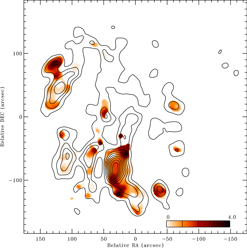
Figure 9: Best estimate of $\tau_{\rm{m}}(1,1)$ in color overlaid on velocity integrated NH₃(1,1) emission in 10% contours (McGary et al., 2001). The opacity map has been smoothed with an eight pixel median filter (see §5). The highest opacity is associated with the southern streamer and the 20 and 50 km s^-1 GMCs while most other features have $\tau_{\rm{m}}(1,1)<1.0$.

When solving for the opacity in the traditional method discussed in §2 we found most gas in our image appeared to have $1<\tau_{\rm{m}}(1,1)<2$. Although this result is in agreement with Coil & Ho (1999, 2000), it is also contrary to our assumption that all rotation inversion transitions of NH₃ are typically optically thin at the Galactic Center. Figure 9 shows our result for $\tau_{\rm{m}}(1,1)$ in color overlaid on 10% contours of NH₃(1,1) velocity integrated emission from McGary et al. (2001). After taking the intrinsic linewidth into account using the method described above, the opacity is no longer biased high by the large observed linewidths and $\langle\tau_{\rm{m}}(1,1)\rangle=0.6$. The opacity is highest along the center of the southern streamer (from ($0^{\prime\prime}$,$-150^{\prime\prime}$) to ($35^{\prime\prime}$,$-75^{\prime\prime}$)). As seen in Figure 9, the southern streamer is the brightest object in our NH₃(1,1) velocity integrated image and is expected to contain $\sim 5\times 10^{4}~{}\rm{M}_{\odot}$ of material (Coil & Ho, 1999). This streamer extends northwards from the 20 km s^-1 GMC towards the nucleus (Ho et al., 1991; Coil & Ho, 1999, 2000). A second extension of the 20 km s^-1 GMC at ($-40$,$-120$) has $\tau_{\rm{m}}(1,1)\approx 1$. The opacity is also elevated in the most northeasterly clump of the 50 km s^-1 GMC. This clump is actually associated with the center of the GMC (to see the full extent of this cloud see Dent et al. (1993)), but is located at the edge of our mosaic where the gain goes to zero (see McGary et al. (2001)). Therefore, the most massive clouds in our maps show the largest opacities as expected.

With these improved estimates of opacity and intrinsic linewidth, the column density and mass could be estimated for each cloud. However, calculation of $N_{(1,1)}$ requires that the peak antenna temperature of the main line, $\Delta T_{A}(1,1)$, be measured for each cloud. In addition, to convert $N_{(1,1)}$ to $N_{\rm{NH}_{3}}$ the rotational temperature of the gas must be known. Because the objective of this paper is to model the effect of large intrinsic linewidths on the line profile and outline the proper method for determining $\Delta\rm{v}_{int}$ and $\tau_{\rm{m}}$, these quantities are not presented in this paper. We will present the calculated $N_{\rm{NH}_{3}}$, $N_{\rm{H}_{2}}$, and cloud masses in a subsequent paper focused on the overall environment in the central 10 pc of the Galaxy. For completeness, we present a brief summary of the method to calculate $N_{(1,1)}$ as well as the average expected value for $N_{(1,1)}$ in this paper.

The excitation temperature, $T_{ex}$, of the gas can be calculated using

$$T_{ex}=2.7~{}\rm{K}+\frac{\Delta T_{A}(1,1)}{1-e^{-\tau_{\rm{m}}(1,1)}}~{}.$$ (10)

This equation assumes a filling factor of 1 and thus produces a lower limit for $T_{ex}$. $T_{ex}$ can then be used to calculate the column density of the main transition using

$$\tau_{\rm{m}}(1,1)=\frac{c^{2}hA_{1-0}f(\nu)N_{1}}{8\pi\nu kT_{ex}}$$ (11)

where $A_{1-0}$ is the Einstein coefficient for spontaneous emission [$1.67\times 10^{-7}$ s^-1 for NH₃(1,1)] and $f(\nu)=(4ln2/\pi)^{\frac{1}{2}}(\Delta\nu)^{-1}$ is the line profile for a Gaussian. $N_{1}$ is the total number in the upper state and is assumed to be equal to $N_{(1,1)}/2$ because the inversion doublet is separated by only $\sim 1$ K. Solving for $N_{(1,1)}$, we find

$$N_{(1,1)}=1.4\times 10^{14}~{}\rm{cm}^{-2}~{}\tau_{\rm{m}}(1,1)T_{ex}\left[\frac{\Delta\rm{v}_{int}}{10~{}\rm{km~{}s}^{-1}}\right]~{}.$$ (12)

Therefore, we expect clouds to have NH₃(1,1) column densities on the order of $10^{14}$ cm^-2 at the Galactic Center. In this paper, we find that $\langle\tau_{\rm{m}}(1,1)\rangle=0.6$ and $\langle\Delta\rm{v}_{int}\rangle=15$ km s^-1. Assuming a lower limit of 7 K for the excitation temperature (Coil & Ho, 1999, 2000), we find a lower limit of $N_{(1,1)}=8.8\times 10^{14}$ cm^-2. Our column density estimate is approximately a factor of five smaller than the typical results of Coil & Ho (1999, 2000), due mostly to the fact that $\langle\tau_{\rm{m}}(1,1)\rangle$ is smaller throughout the region when the effects of large intrinsic linewidths are removed. As long as the gas is optically thin, the effect of the filling factor on the measured column density is minimized. In this case, small clumps of gas with a large column density is essentially equivalent to gas with a larger filling factor and a smaller column density.

Figure 10 shows that the correlation between $\tau_{\rm{m}}(1,1)$ and $\Delta\rm{v}_{int}$ after the application of our method resembles a scatter plot. The correlation coefficient is –0.14, compared to 0.69 in Figure 2$b$. By considering the effect of blending, we have successfully modeled the observed linewidth and calculated accurate intrinsic linewidths and opacities. Finally, it is important to note that the spread in $\Delta\rm{v}_{int}$ is very similar to the spread in $\Delta\rm{v}_{obs}(3,3)$. Therefore, one may assume that observations of NH₃(3,3) give a good indication of the intrinsic linewidth of the gas and corrections need not be applied in general.

6 Conclusion

In gas with large intrinsic linewidths, the five quadrupole hyperfine components of the NH₃ rotation inversion transitions will blend into a single-line profile. The observed linewidth will greatly overestimate $\Delta\rm{v}_{int}$ and bias the opacity to high values. We model the effect of $\Delta\rm{v}_{int}$ on observed NH₃(1,1), (2,2), and (3,3) linewidths for a range of opacities. A detailed method for recovery of the intrinsic linewidth and opacity using $\Delta\rm{v}_{obs}$ and the intensity of two NH₃ rotation inversion transitions is then presented. We focus on the case where only the observed linewidth of the profile is known which makes the method particularly useful for correcting historical data for which the exact line profiles are not readily available. Application of this method to our data from the central 10 pc of the Galaxy results in the first independent measures of the opacity and intrinsic linewidth of NH₃(1,1) near the nucleus. The calculated intrinsic linewidths when blending is accounted for are reduced by a factor of $\sim 2$ from the initial observed linewidths to $\langle\Delta\rm{v}_{int}\rangle=15$ km s^-1 and now agree with the other molecular tracers in the region, including NH₃(3,3). Gas along the edge of Sgr A East or in close projected distance to the nucleus appears to have increased intrinsic linewidths. All except the most massive clouds in our images show $\tau_{\rm{m}}(1,1)<1$. This confirms the observation that even the lowest energy transitions are less affected by self-absorption than HCN(1-0) and HCO⁺(1-0).

Table 1: Parameters for NH₃ Rotation Inversion Transitions

			Inner Hyperfine		Outer Hyperfine
Transition	Frequency	Energy	$\Delta$v	Theoretical	$\Delta$v	Theoretical
	(GHz)	K	(km s-1)	Intensity	(km s-1)	Intensity
NH3(1,1)	23.694495	23.4	7.7	0.278	19.3	0.222
NH3(2,2)	23.722633	64.9	16.5	0.0628	25.7	0.0652
NH3(3,3)	23.870129	124.5	21.4	0.0296	28.8	0.0300

Figure 1: Line profiles for NH₃(1,1) for $\tau_{\rm{m}}\ll 1$ and $\Delta\rm{v}_{int}=1$, 5, 10, and 15 km s^-1. As $\Delta\rm{v}_{int}$ increases, the five electric quadrupole hyperfine components blend into one single line.

Figure 2: $a)$ Observed NH₃(1,1) linewidth, $\Delta\rm{v}_{obs}(1,1)$, as a function of $\tau_{\rm{m}}(1,1)$ for all points in our data where the flux was bright enough to fit for both parameters. The strong correlation indicates that blending due to large linewidths has corrupted our results such that an increase in observed linewidth also appears as an increase in opacity. The correlation between adjacent points in the plot is the result of many samplings per beam ($\theta_{b}=15^{\prime\prime}$). $b)$ Same as $a$, but the data were first averaged over a single beam and the resulting values for $\tau_{\rm{m}}(1,1)$ and $\Delta\rm{v}_{obs}$ are plotted. The correlation between $\tau_{\rm{m}}(1,1)$ and $\Delta\rm{v}_{obs}$ is still easily observable and has a correlation coefficient of 0.69.

Figure 3: Observed NH₃(3,3) linewidth, $\Delta\rm{v}_{obs}(3,3)$, as a function of $\tau_{\rm{m}}(3,3)$ for all points in our data where the flux was bright enough to fit for both parameters. The correlation is less strong than in Figure 2 and has a correlation coefficient of 0.07.

Figure 4: $a)$Observed linewidth as a function of intrinsic linewidth for NH₃(1,1), (2,2), and (3,3) for $\tau_{\rm{m}}\ll 1$. The dashed line shows $\Delta\rm{v}_{obs}=\Delta\rm{v}_{int}$. Note that the observed linewidth of NH₃(1,1) will greatly overestimate $\Delta\rm{v}_{int}$ for $\Delta\rm{v}_{int}>5$ km s^-1. $b)$ $\Delta\rm{v}_{obs}/\Delta\rm{v}_{int}$ for $\Delta\rm{v}_{int}\leq 60$ km s^-1 for NH₃(1,1), (2,2), and (3,3) for $\tau_{\rm{m}}\ll 1$.

Figure 5: $a)$ Line profiles of NH₃(1,1) for $\tau=0.01$, 1.0 and 5.0 for $\Delta\rm{v}_{int}=3$ km s^-1. In this case, there is no blending so a fit of a Gaussian to the main line will give a good estimate of $\Delta\rm{v}_{int}$ (see Figure 6$a$). $b)$ Same as $a$, but for $\Delta\rm{v}_{int}=15$ km s^-1. In this case, the hyperfine components are highly blended and an increase in $\tau_{\rm{m}}(1,1)$ will greatly affect the observed linewidth.

Figure 7: Observed NH₃(1,1) linewidth as a function of $\tau_{\rm{m}}(1,1)$ for a range of $\Delta\rm{v}_{int}$.

Figure 10: Intrinsic linewidth, $\Delta\rm{v}_{int}$, as a function of $\tau_{\rm{m}}(1,1)$ after application of our correction method. Averages over the 15^′′ beam have been taken as in Figure 2$b$ and the correlation coefficient is only -0.14.

References

- Armstrong & Barrett (1985) Armstrong, J.T. & Barrett, A.H. 1985, ApJS, 57, 535
- Barranco & Goodman (1998) Barranco, J.A. & Goodman, A.A. 1998, ApJ, 504, 207
- Coil & Ho (1999) Coil, A.L. & Ho, P.T.P. 1999, ApJ, 513, 752
- Coil & Ho (2000) Coil, A.L. & Ho, P.T.P. 2000, ApJ, 533, 245
- Dent et al. (1993) Dent, W.R.F, Matthews, H.E., Wade, R. , & Duncan, W.D. 1993, ApJ, 410, 650
- Eckart & Genzel (1997) Eckart, A. & Genzel, R. 1997, MNRAS, 284, 576
- Genzel et al. (1990) Genzel, R., Stacey, G.J., Harris, A.I., Geis, N., Graf, U.U., Poglitsch, A. , & Sutzki, J. 1990, ApJ, 356, 160
- Genzel & Townes (1987) Genzel, R. & Townes, C.H. 1987, ARA&A, 25, 377
- Ghez et al. (1998) Ghez, A.M., Klein, B.L., Morris, M. , & Becklin, E.E. 1998, ApJ, 509, 678
- Güsten, Walmsley, & Pauls (1981) Güsten, R., Walmsley, C.M. , & Pauls, T. 1981, A&A, 103, 197
- Güsten & Downes (1980) Güsten, R. & Downes, D. 1980, A&A, 87, 6
- Ho (1977) Ho, P.T.P. 1977, Ph.D. thesis, Massachusetts Institute of Technology
- Ho et al. (1991) Ho, P.T.P., Ho, L.C., Szczepanski, J.C., Jackson, J.M., Armstrong, J.T. , & Barrett, A.H. 1991, Nature, 350, 309
- Ho et al. (1977) Ho, P.T.P., Martin, R.N., Myers, P.C., & Barrett, A.H. 1977, ApJ, 215, 29
- Ho et al. (1990) Ho, P.T.P., Martin, R.N., Turner, J.L., & Jackson, J.M. 1990, ApJ, 355, 19
- Ho & Townes (1983) Ho, P.T.P. & Townes, C.H. 1983, ARA&A, 21, 239
- Maeda et al. (2001) Maeda, T. et al. 2001, astro-ph/0102183
- McGary et al. (2001) McGary, R.S., Ho, P.T.P., & Coil, A.L. 2001, ApJ, 559, 326
- Mezger et al. (1989) Mezger, P.G., Zylka, R. Salter, C.J., Wink, J.E., Chini, R. Kreysa, E. , & Tuffs, R. 1989, A&A, 209, 337
- Reid (1993) Reid, M.J. 1993, ARA&A, 31, 345
- Serabyn, Lacy, & Achtermann (1992) Serabyn, E., Lacy, J.H. , & Achermann, J.M. 1992, ApJ, 395, 166
- Townes & Schalow (1975) Townes, C.H. & Schalow, A.L. 1975, Microwave Spectroscopy, New York:Dover
- Zylka (1999) Zylka, R., Güsten, R., Philipp, S., Ungerechts, H., Mezger, P.G. , & Duschl, W.J. 1999, in ASP Conf. Ser, 186, The Central Parsecs of the Galaxy, ed. H. Falcke et al. (San Francisco: ASP), 415
- Yusef-Zadeh & Morris (1987) Yusef-Zadeh, F. & Morris, M. 1987, ApJ, 320, 545