Abstract

I review the recent developments in the analysis of cosmic flow data, in particular, latest results of bulk flow measurements, comparison between redshift and peculiar velocity catalogs with emphasis on the measured value of the $\beta\,(=\Omega_{m}^{0.6}/b)$ parameter, and matter power spectrum estimates from galaxy peculiar velocity catalogs. Based on these developments, one can argue that most of the previous discrepancies in the interpretation of cosmic flow data, maybe with the exception of bulk flow measurements on scales $\lower 2.15277pt\hbox{$\;\buildrel>\over{\sim}\;$}100h{{}^{-1}}{\rm Mpc}$, have either been resolved or fairly understood.

Cosmic Flows: Review of Recent Developments

Max Planck Institute for Astrophysics
Karl-Schwarzschild-Str. 1
D-85741 Garching, Germany

0.1 Introduction

Within the gravitational instability (GI) framework for the growth of cosmic structures, the peculiar velocity field of galaxies and clusters provides a direct and reliable probe of the matter distribution, under the natural assumption that these objects are unbiased tracers of the large-scale, gravitationally induced, velocity field. The GI paradigm requires that the linear peculiar velocity, ${\bf v}({\bf r})$ – defined as the deviation from Hubble expansion – and linear mass density contrast, $\delta_{m}({\bf r})$, be related to one another according to the local (differential) relation,

$$\nabla\cdot{\bf v}=-\Omega_{m}^{0.6}\delta_{m},$$ (1)

or its global (integral) counterpart,

$${\bf v}={\Omega_{m}^{0.6}\over 4\pi}\int d^{3}{\bf r^{\prime}}{\delta_{m}({\bf r^{\prime}})({\bf r^{\prime}}-{\bf r})\over|{\bf r^{\prime}}-{\bf r}|^{3}},$$ (2)

where $\Omega_{m}$ is the matter overdensity parameter. Note that the peculiar velocity field is determined by the distribution of the matter with all its components especially the dominant dark matter component.

In order to measure peculiar velocities of galaxies and clusters, observers use a variety of distance indicators. Generally, these indicators relate two quantities, one among which is distance dependent, e.g., galaxy luminosity, and the other is distance independent, e.g., galaxy rotational velocity. The best known examples of such indicators are the Tully-Fisher [24] and Faber-Jackson [13] relations; over the last decade or so these and many other types of distance indicators have been used to measure cosmological distances. The availability of a large number of galaxy peculiar velocity catalogs, some of them with few thousands objects, have turned cosmic flows to one of the main probes used to study the large scale structure in the nearby universe. Here I’ll concentrate on the following three statistical measures of the velocity field:

1. The Bulk Flow: This measure, defined as the average streaming motion within certain volume, is probably the easiest statistic to estimate from the observed radial component of peculiar velocities. At the Cosmic Microwave Background radiation (CMB) restframe, the bulk motions are expected to converge to zero with increasing volume. The rate of convergence depends on the fluctuations in the matter distribution on various scales, i.e., the large scale matter fluctuations power spectrum. This dependence on cosmological models has motivated several attempts to measure the dipole component of the local peculiar velocity field and to determine the volume within which the streaming motion vanishes. As of yet, bulk flow measurements have produced conclusive and consistent results only on scales $\lower 2.15277pt\hbox{$\;\buildrel<\over{\sim}\;$}60h{{}^{-1}}{\rm Mpc}$, but failed to do so on scales $\lower 2.15277pt\hbox{$\;\buildrel>\over{\sim}\;$}100h{{}^{-1}}{\rm Mpc}$ (for recent works see [4, 5, 8, 9, 15, 17, 26]).

2. The mass power spectrum: Equation 2 suggests that one can estimate the bias free, $\Omega_{m}^{1.2}$ weighted, matter power spectrum directly from the measured peculiar velocities. To date, likelihood analysis based estimations of the matter power spectrum exist for the Mark III [35], SFI [14] and ENEAR [31] catalogs. All of these measurements has consistently produced power spectra with amplitudes larger than those measured by other data sets, e.g., galaxy redshift surveys.

3. The $\beta$ parameter: Peculiar velocities enable a reconstruction of the large scale matter distribution independent of redshift surveys. Therefore, one can use Eqs. 1 and 2 to compare the matter and 3D velocity distributions deduced from the measured radial peculiar velocities to those obtained from redshift surveys. This comparison requires biasing model which specifies how galaxies follow the underlying total matter distribution. On the scales of interest, it is usually assumed that

   $$\delta_{g}=b\delta_{m},$$ (3)

   where $\delta_{g}$ is the galaxy observed density contrast and $b$ is the linear bias parameter. The comparison is used to: 1) test the validity of Eqs. 1 and 2, namely, the basic GI paradigm; 2) test the linear biasing model; 3) directly measure the value of $\Omega_{m}$ ([3, 7, 10, 21, 28, 29] and [32]). Until recently, comparisons using Eq. 1 have systematically yielded $\beta$ values larger than those obtained from using Eq. 2.

As mentioned above, many have attempted to estimate these statistical measures of peculiar velocities over the years. Until recently, the results they obtained have often been inconsistent with each other and with estimations from other data, depending on the specific peculiar velocity catalog at hand and the analysis methods. It is generally accepted that the main reason for the inconsistencies lies in the problematic nature of the distance indicators used to determine the peculiar velocities. First, the distance measurements carry large random errors, including intrinsic scatter in the distance indicator and measurement errors, which grow in proportion to the distance from the observer and thus become severe at large distances. Further nontrivial errors are introduced by the nonuniform sampling of the galaxies that serve as velocity tracers. In particular, the Galactic disk obscures an appreciable fraction of the sky, creating a significant“zone of avoidance” of at least $40\%$ of the sky. When translated to an underlying smoothed field, these errors give rise to severe systematic biases. In light of these difficulties, the inconclusive results have led many to question the reliability of the peculiar velocity datasets as cosmological probes.

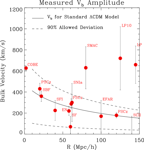
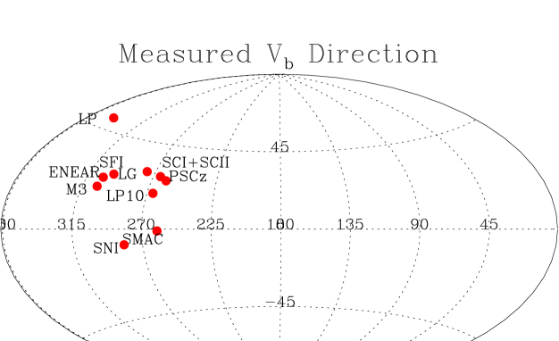
Figure 1: Bulk Flow measurements. Upper panel: the symbols show the amplitude of the measured bulk flow (with its error) from the following surveys: Surface Brightness Fluctuations (SBF), SFI , ENEAR (EN), Shellflow (SF), Supernovae type Ia (SNIa), SMAC, EFAR, LP10, SCII and LP (see table for explanation) as a function of radius. The CMB dipole COBE measurement and bulk flow from the PSC$z$ redshift catalog are also shown. The solid line shows the expected rms bulk velocity of a sphere of radius $R$ for standard $\Lambda$CDM model; the dashed lines represent 1-$\sigma$ cosmic scatter about the rms. Lower panel: the symbols show the direction of some of the measured bulk flow vectors, note that the catalogs that correspond to $R\sim 60h{{}^{-1}}{\rm Mpc}$ have consistent directions while measurements that correspond to large distances do not.

In this article, I review the recent developments in these three areas and show that significant improvements have occurred in the field in the past few years. In addition, an argument is put forward that those developements lead to alleviating most of the inconsistencies and to understanding, at least qualitatively, the cause of the remaining outstanding ones.

0.2 Bulk Flow

The bulk flow motion direction and amplitude on different scales are the simplest quantities to measure from peculiar velocity data. They provide constraints on the power-spectrum of mass fluctuations. Theoretically, the mean square bulk velocity within a sphere of radius $R$, is given by,

$$\langle v^{2}(R)\rangle={\Omega_{m}^{1.2}\over 2\pi^{2}}\int_{0}^{\infty}P(k)\tilde{W}^{2}(kR)dk,$$ (4)

where $P(k)$ is the mass fluctuation power spectrum and $\tilde{W}(kR)$ is the Fourier transform of a top-hat window of radius R. In the upper panel of Figure 1 the rms expected bulk velocity, ${V_{b}}^{rms}(R)=\sqrt{\langle v^{2}(R)\rangle},$ is plotted against R for a standard $\Lambda$CDM power spectrum with the dashed lines representing the $1\sigma$ cosmic scatter deviations expected within the given volume. Note that the large cosmic scatter weakens the bulk flow statistic as a probe of cosmological models.

On the observational side one can divide the currently available measurements into two main domains. The first is measurements of ${\bf V}_{b}$ within radius $\lower 2.15277pt\hbox{$\;\buildrel<\over{\sim}\;$}60h^{-1}Mpc$. Bulk flow values within this radius as measured from the SFI [6], Mark III [12] and the recently completed Shellflow [8] and ENEAR [5] catalogs, lead to a roughly consistent picture even though some discrepancies still remain. For instance, the Mark III catalog yields a systematically larger amplitude of the bulk motion $\sim 370$ ${\rm km\,s{{}^{-1}}}$ on scales $\sim 60h{{}^{-1}}{\rm Mpc}$ as compared to values of $\lower 2.15277pt\hbox{$\;\buildrel<\over{\sim}\;$}220$ ${\rm km\,s{{}^{-1}}}$ obtained from the other catalogs; this specific discrepancy is probably caused by the calibration problem the Mark III catalog is known to suffer from [8, 10].

Recently, results from the long awaited Surface Brightness Fluctuations (SBF) method have been first published [23]. They give a bulk flow value of $350{\rm km\,s{{}^{-1}}}$ at $30h{{}^{-1}}{\rm Mpc}$ distance. The bulk flow measurement within this volume, both in terms of amplitude and direction, is consistent with what is known about the structures just outside the sampled volume, e.g., the Great-Attractor the Perseus-Pisces superclusters.

The second domain is measurements within $R\lower 2.15277pt\hbox{$\;\buildrel>\over{\sim}\;$}100h{{}^{-1}}{\rm Mpc}$. The results here are far from being conclusive and various data sets lead to different bulk flow amplitudes and directions. While there is supporting evidence pointing towards convergence of the bulk flow on these large scales [9, 20, 4], other works [19, 26, 17] argue for the existence of large amplitude ($\lower 2.15277pt\hbox{$\;\buildrel>\over{\sim}\;$}600$ ${\rm km\,s{{}^{-1}}}$) streaming motions out to a depth as large as $150h{{}^{-1}}{\rm Mpc}$, ruling out that the Hubble flow has converged to the CMB frame at smaller distances. Given the far reaching implications that these large-scale motions would have on currently popular cosmological models it is clear that this issue is of great interest. It is important to point out, however, that the direction and the amplitude of the bulk motion detected on large scales by different authors do not agree with each other. Additional independent bulk flow estimates, e.g., from the PSC$z$ redshift catalog and more recently from the dipole of the NVSS radio sources [2], are consistent with bulk flow convergence in the CMB restframe (see upper panel of Fig. 1).

A summary of the bulk flow measurements is given in Fig. 1 and Table 1.

Table 1: Recent Bulk Flow Measurements

Survey	$V_{b}$	R	Comments
	(${\rm km\,s{{}^{-1}}}$ )	($h^{-1}{\rm Mpc}$ )
Tonry et al. [23]	$350$	$30$	SBF∗
Dekel et al. [12]	$370$	$60$	M3⋆ (TF† + $D_{n}-\sigma$)
Giovanelli et al. [15]	$200$	$60$	SFI (TF)
Courteau et al. [8]	$70$	$60$	Shellflow (TF)
da Costa et al. [5]	$220$	$60$	ENEAR ($D_{n}-\sigma$)
Riess et al. [20]	$\approx 0$	$100$	SNIa∙
Colless et al. [4]	$\approx 0$	$\sim 100$	EFAR (FP⋄)
Hudson et al. [17]	$600$	$140$	SMAC (FP)
Lauer & Postman [19]	$700$	$150$	LP (BCG‡)
Willick [26]	$700$	$150$	LP10K (TF)
Dale et al. [9]	$\approx 0$	$\sim 150$	SCI/SCII (TF)

^∗ Surface Brightness Fluctuations method. ^⋆ Mark III dataset. ^† Tully-Fisher Measurement. ^∙ Supernovae type Ia. ^⋄ Fundamental Plane measurement. ^‡ Brightest Cluster Galaxy method.

0.3 Power Spectrum Analysis

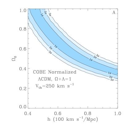
Figure 2: Contour map of ln-likelihood in the $h-\Omega$ plane for $\Lambda$CDM models with $250$ ${\rm km\,s{{}^{-1}}}$ thermal error component (added to account for the nonlinear environment in which early type galaxies tend to reside). The contours denote the most likely values within $1,2$ and $3\sigma$ confidence levels.

The matter power spectrum has been measured from the Mark III [18, 35], SFI [14] and ENEAR [31] catalogs. With the exception of one study [18], all the power spectrum estimations apply likelihood analysis which assumes that both the underlying velocity field and the errors are drawn from independent random Gaussian fields. The observed peculiar velocities constitute a multi-variant Gaussian data set, albeit the sparse and inhomogeneous sampling; this probability distribution function is reinterpreted as a likelihood function of the measured radial velocities given a model power spectrum. Maximizing the likelihood with respect to the model free parameters yields a best fit power spectrum.

Together with its advantages (no explicit window function, weighting or smoothing the data and automatic underweighting of noisy, unreliable data) the likelihood method requires satisfying the following conditions: 1) explicit knowledge of the distribution function; 2) peculiar velocities are related to the over-densities through linear theory; 3) errors in the inferred distances constitute a Gaussian random field with scatter that scales linearly with distance. In addition, the likelihood analysis requires assuming a parametric functional form for the power spectrum.

A typical result of the power spectrum parameters as estimated from, for example, the ENEAR data is presented in Fig. 2. This figure shows the likelihood contour map in the $\Omega_{m}-h$ plane, for the $\Lambda$CDM family of models with Harrison-Zeldovich spectrum ($n=1$). In addition to the normal, distance dependent, uncertainties the error matrix is assumed here to have a diagonal random contribution of $250$ ${\rm km\,s{{}^{-1}}}$ that accounts for the nonlinear environment within which the ENEAR early-type galaxies prefertionaly reside. The most probable parameters in this case (in the range $\Omega_{m}\leq 1$) are $\Omega_{m}=1$ and $h=0.5$. The elongated contours clearly indicate that neither $\Omega_{m}$ nor $h$ are independently well constrained. It is rather a degenerate combination of the two parameters, approximately $\Omega_{m}h^{x}$ with $x\sim 1$ that is being determined tightly by the elongated ridge of high likelihood.

As pointed out earlier, the power spectrum amplitude deduced from galaxy peculiar velocity data is considerably higher than those obtained from other types of data sets, usually favor the standard $\Lambda$CDM model ($\Omega_{m}=0.3$, $\Lambda=0.7$ and $h=0.65$). This naturally raises the question of whether is the discrepancy driven by a yet undetected systematic effect in the data, or by something deeper?

It is important to point out that the power spectrum estimation method is very sensitive to the assumed small scale power model (induced by noise and/or nonlinear evolution) which can add or suppress power. Recently, Hoffman and Zaroubi [16] have carried out a detailed inspection of the goodness-of-fit of the Mark III, SFI, and ENEAR best-fit power spectra by using Principal Component Analysis (PCA) approach and found that in neither of the three cases do the assumed theoretical power spectrum and/or error model give an acceptable fit. In a subsequent study, Silberman et al. [22] have shown that this misfit is probably caused by ignoring small scale power in the analysis; thereby casting a large shadow of doubt about the applicability of the error models or the strict validity of linear dynamic, assumed so far.

0.4 The Value of $\beta$

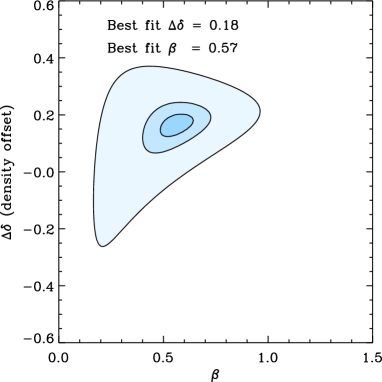
Figure 3: $\beta$ from density-density comparison. Left Panel: The 1, 2 and 3 $\sigma$ likelihood contours in the $\beta-\Delta\delta$ plane. Right Panel: A scatter plot showing the SEcat UMV reconstructed G12 density vs. the PSC$z$ G12 density. In this comparison, one out of ten from all the data points that have reconstruction error $<0.2$ was randomly picked. The size of the symbols is inversely proportional to their errors.

Galaxy peculiar velocities and their redshift space positions have been used to estimate the value of $\beta=\Omega_{m}^{0.6}/b$, under the hypotheses of linear theory and linear biasing. These analyses have been typically carried out using two alternative strategies. In the so-called density-density comparisons a 3-D velocity field and a self-consistent mass density field are derived from the observed radial velocities and compared to the galaxy density field measured from large redshift surveys, under the assumption of linear bias (a combination of Eqs. 1 & 3). The typical example here is the comparison of the density field reconstructed applying the POTENT method [1, 11] to the MARK III catalog of galaxy peculiar velocities [27] with the IRAS 1.2 Jy redshift catalog density field [21]. The various applications of density-density comparisons to a number of datasets have persistently led to large estimates of $\beta$, consistent with unity [21]. The alternative approach is that of the velocity-velocity analysis. In this second case the observed galaxy distribution is used to infer a mass density field from which peculiar velocities are obtained and compared to the observed ones (a combination of Eqs. 2 & 3). The velocity-velocity methods have been applied to most catalogs presently available yielding systematically lower values of $\beta$, in the range of $0.4-0.6$.

Both density-density and velocity-velocity methods have been carefully tested using mock catalogs extracted from N-body simulations. They were shown to provide an unbiased estimate of the $\beta$ parameter. Yet, when applied to the same datasets the discrepancy in the $\beta$ estimates turned out to be significantly larger than the expected errors. Velocity-velocity comparisons are generally regarded as more robust as they require manipulation of redshift catalog data as opposed to the density-density comparison which manipulates the noisier and sparser peculiar velocity data. In any case both approaches are quite complicated and it is hard to understand how systematic errors can arise and propagate through the analysis. It is, therefore, likely that these systematic effects do influence the $\beta$ parameter estimation.

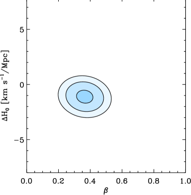
Figure 4: $\beta$ from velocity-velocity comparison. Left Panel: The 1,2, and 3 $\sigma$ likelihood contours in the $\beta-\Delta H_{\circ}$ plane from a comparison of the SEcat G12-smoothed radial velocities at the locations of the SEcat data points vs. the PSC$z$ G12-smoothed radial velocities at the same locations comparison. Right Panel: A scatter plot of the G12-smoothed radial velocities, in this comparison all data points have been included. The size of the symbols is inversely proportional to the errors

Since all the previous results have been obtained with methods designed to conclusively carry out either velocity-velocity comparison (ITF [10] & VELMOD [28, 29]) or density-density comparison (POTENT [21]), it is very difficult to know whether the source of the discrepancy is data or methodology driven. Recently, a new linear approach, called unbiased minimal variance (UMV) method has been proposed [30]. With the UMV method, both velocity-velocity and density-density comparisons can be carried out within the same methodological framework.

Similar to the Wiener Filter [25, 34], the UMV estimator is derived by requiring the linear minimal variance solution given the data and an assumed prior model specifying the underlying field covariance matrix. However, unlike the Wiener filter, the minimization is carried out with the added constraint of an unbiased reconstructed mean field. In the context of reconstruction from peculiar velocity data, the UMV algorithm could be regarded as a compromise between the POTENT algorithm, which assumes no regularization but might be unstable to the inversion problem of deconvolving highly noisy data, and the Wiener filter algorithm, which takes into account the correlation between the data points and therefore stabilizes the inversion, but constitutes a biased estimator of the underlying field (for detailed discussion see [30, 32]).

The UMV approach has been applied to the SFI, ENEAR, Mark III and to the newly compiled SEcat catalog (which is a combination of the SFI and ENEAR catalogs) [32]. The reconstructed fields are compared with those predicted from the IRAS PSC$z$ galaxy redshift survey to constrain the value of $\beta$. For example, the analysis of the SEcat catalog for the first time leads to consistent $\beta$ values from the comparison of the density and the velocity fields yielding $\beta=0.57_{-0.13}^{+0.11}$ and $\beta=0.51\pm{0.06}$, respectively. The $\beta$ values obtained from comparing the PSC$z$ data to each of the four galaxy peculiar velocity catalogs are consistent.

Table 2: $\beta$ Measurements

Method	Compared data	$\beta$
	$\delta-\delta$ Comparison
POTENT [21]	Mark III vs. IRAS 1.2Jy	$0.89\pm 0.12$
UMV[32]	SEcat vs. PSCz	$0.57^{+0.11}_{-0.13}$
	$v-v$ Comparison
VELMOD [29, 28]	Mark III vs. IRAS 1.2Jy	$0.50\pm 007$
VELMOD [3]	SFI vs. PSCz	$0.42\pm 0.07$
ITF [10]	Mark III vs. IRAS 1.2Jy	$?^{\dagger}$
ITF [7]	SFI vs. IRAS 1.2Jy	$0.6\pm 0.1$
UMV [32]	SEcat vs. PSCz	$0.51\pm 0.06$

^† Inconsistent flow fields (probably due to problematic calibration of Mark III)

Figure 3 shows the estimated value of $\beta$ from the PSC$z$ and the SEcat density-density comparison. The fields where smoothed with $12h{{}^{-1}}{\rm Mpc}$ Gaussian kernel; only points with small errors, estimated from Monte Carlo mock SEcat realizations, where used in the comparison. The left panel shows a contour plot in the plane of $\beta$ and $\Delta\delta$ which corresponds to zero-point density offset. The 1, 2 and 3-$\sigma$ level certainty contours are shown. These contours are drawn assuming that the error in the density at each individual point is independent, this assumption is obviously wrong. Therefore, in the $\beta$ results quoted in the previous paragraph the uncertainty has been estimated by adding, in quadrature, to the likelihood analysis 1-$\sigma$ uncertainties the error in recovering $\beta$ as estimated from the Monte Carlo simulations. The right panel shows a scatter plot of densities with their best fit linear model. Figure 4 shows results similar to the previous figure, but for the reconstructed radial velocity field. The comparison here is somewhat different in the sense that it is carried out between the reconstructed $12h{{}^{-1}}{\rm Mpc}$ smoothed radial velocities at the location of the SEcat data points. For more details on the comparison see [32].

Summary of the $\beta$ parameter values obtained from various velocity-velocity and density-density comparisons is shown in table 2.

Although, the results obtained by the UMV analysis strengthen the case for lower $\beta$ values, by no account do they render the results of the Mark III-POTENT analysis invalid. However, they call for re-examination of the later bearing in mind the following issues. The Mark II catalog, as shown for example by Davis et al. [10] and more recently by Courteau et al. [8], suffers from systematic calibration error that would cause a systematic error in the estimation of $\beta$. However, this error is not expected to affect the density-density comparison as to overestimate the value of $\beta$ by more than a factor of two. An application of the UMV method to the Mark III catalog [32] shows that the obtained values of $\beta$ are much lower than those obtained by applying the POTENT analysis [21] but still they are somewhat higher than those obtained from the SEcat catalogs by $0.1-0.2$. Moreover, the velocity-velcotiy analysis (like VELMOD) yield consistent values of $\beta$ when applied to Mark III and SFI datasets [3, 28, 29]. Based on these arguments, one could speculate that the most likely explanation to the previous inconsistency is a result of a collusion between the systematic errors in Mark III and the noise sensitivity of the POTENT reconstruction.

0.5 Summary & Discussion

To evaluate the outstanding issues in the peculiar velocity measurements in general terms one should differentiate between two types of problems. The first is the inconsistencies among results obtained from various peculiar velocity data sets and occasionally even within those obtained from the same data set. The second, is the disagreement with measurements from other types of data sets. The former is obviously more severe as it implies unresolved systematics in the peculiar velocity datasets themselves. Measuring by this yard stick, the conflicting results obtained from the bulk flow and the $\beta$ parameter measurements are more serious than the higher amplitude found with the power spectrum measurements.

It is reassuring that within the local universe ($R\lower 2.15277pt\hbox{$\;\buildrel<\over{\sim}\;$}60h{{}^{-1}}{\rm Mpc}$) all the recent bulk flow measurements, especially from the SFI, Shellflow and ENEAR catalogs do agree very well with each other both in terms of amplitude and direction. Those three marginally agree with the Mark III data, which gives a somewhat higher value of $V_{b}$. Given that the Shellflow sample have clearly shown that the Mark III data set is somewhat miscalibrated, this disagreement is hardly an issue.

Unfortunately however, the picture on larger scales ($R\lower 2.15277pt\hbox{$\;\buildrel>\over{\sim}\;$}100h{{}^{-1}}{\rm Mpc}$) is very different and the disagreement among the various measurements is yet to be resolved. While the bulk flow obtained from the SNIa [20], SCI/SCII [9] and EFAR [4] samples clearly points toward convergence of the CMB dipole; the SMAC[17], LP [19] and LP10 [26] surveys find a bulk flow amplitude of $\sim 600-700{\rm km\,s{{}^{-1}}}$. Although the former three measurements are consistent with the one obtained from the PSC$z$ redshift catalog data, the NVSS radio sources and with theoretical prejudice, by no means the later three have been refuted. It is worth pointing out however, that the LP bulk flow, while comparable in amplitude, disagrees with the SMAC and LP10 flow. Furthermore, almost all of the deep peculiar velocity surveys have small number of objects and therefore probably prone to the pitfalls of small number statistics.

The peculiar velocity measurements have systematically led to mass power spectrum amplitudes higher than those obtained from other types of data. In light of the overwhelming evidence pointing towards lower amplitude power spectrum, a special effort should be made to rule out any inherent bias in the prior assumptions made in the peculiar velocity based power spectrum measurements. In fact, two recent studies [16, 22] strongly suggest a generic problem with the theoretical framework used to estimate the mass power spectrum from the Mark III, SFI, and ENEAR velocity surveys. Possible sources of this problem lie with non-linear dynamical effects and/or oversimplified treatment of errors [22].

The irreconcilability of the $\beta$ estimation from density-density and velocity-velocity comparisons has been one of the major outstanding issues in the cosmic flows field of study. A new technique, the UMV, have enabled carrying out, for the first time, both comparisons in the same framework. The results obtained by applying this technique to several galaxy peculiar velocity catalogs yield low values of the $\beta$ parameter ($\sim 0.5-0.6$), a result consistent with those obtained from the previous velocity-velocity comparisons and from the analysis of redshift surveys. These latest results clearly strengthen the case for low $\beta$ values, in agreement with those obtained by the previous velocity-velocity studies. A qualitative inspection into the reason of the discrepancy in the estimation of $\beta$ between the UMV and POTENT density-density comparisons allows one to speculate that the most likely explanation is a collusion between both the systematic errors in the Mark III data and the noise effects on the POTENT algorithm, that somehow conspired to produce these high $\beta$-values.

In light of the developments presented in this review, it is argued that most of the outstanding issues in the large scale peculiar velocity field of study, maybe with the exception of the large scale velocity field, have been either resolved or understood (at least qualitatively) and we finally have a consistent cosmological model emerging from the study of cosmic flows. The experience gained during the convergence towards the current status, despite the crooked path it took, will be invaluable when dealing with the large future datasets.

Acknowledgements

Much of the work presented here have been done in collaboration with E. Branchini, L.N. da Costa and Y. Hoffman, their contribution is acknowledged. I would like to thank the organizers of this meeting for suggesting to me to review this topic.

Bibliography

- [1] Bertschinger E., Dekel A. 1989, ApJ, 336, L5
- [2] Blake, C., Wall, J., 2002, Nature, 416, 150.
- [3] Branchini E., Freudling, W. da Costa L., Frenk C., Giovanelli R., Haynes M., Salzer J., Wegner G., Zehavi I. 2001, MNRAS, 326, 1191.
- [4] Colless, M., Saglia, R. P., Burstein, D., Davies, R. L., McMahan, R. K., Wegner, G., 2001, MNRAS, 321, 277
- [5] da Costa, L.N., Bernardi, M., Alonso, M.V., Wegner, G., Willmer, C.N.A., Pellegrini, P.S., Maia, M.A.G., Zaroubi, S., ,2000, ApJ, 537, L81
- [6] da Costa, L. N., Freudling, W., Wegner, G., Giovanelli, R., Haynes, M. P., & Salzer, J. J. 1996, ApJ, 468, L5
- [7] da Costa L., Nusser, A., Freudling W., Giovanelli R., Haynes M., Salzer J. Wegner G. 1998, MNRAS, 299, 452
- [8] Courteau, S., Willick, J.A., Strauss, M.A., Schlegel, D., & Postman, M. 2000, ApJ, 544, 636
- [9] Dale, D. A., Giovanelli, R., Haynes, M. P., Campusano, L. E., Hardy, E., & Borgani, S. 1999, ApJ, 510, L11
- [10] Davis, M., Nusser, A., Willick, J.A., 1996, ApJ, 473, 22.
- [11] Dekel A., Bertschinger E. & Faber S.M. 1990, ApJ, 364, 349
- [12] Dekel, A., Eldar, A., Kolatt, T., Yahil, A., Willick, J. A., Faber, S. M., Courteau, S., Burstein, D., 1999, ApJ, 522, 1
- [13] Faber, S. M., Jackson, R. E., 1976, ApJ, 204, 668.
- [14] Freudling, W., Zehavi, I., da Costa, L.N., Dekel, A., Eldar, A., Giovanelli, R., Haynes, M.P., Salzer, J.J., Wegner, G., & Zaroubi, S. 1999, ApJ, 523, 1.
- [15] Giovanelli R., Haynes M., Herter T., Vogt N., da Costa L., Freudling W., Salzer J., Wegner G. 1997, AJ, 113, 53
- [16] Hoffman, Y. and Zaroubi, S., 2000, ApJL, 535, L5.
- [17] Hudson, M.J., Smith, R.J., Lucey, J.R., Schlegel, D.J., & Davies, R.L. 1999, ApJ, 512, L79
- [18] Kolatt, T., & Dekel, A. 1997, ApJ, 479, 592
- [19] Lauer, T. R., & Postman, M. 1994, ApJ, 425, 418
- [20] Riess, A.G., Davis, M., Baker, J., & Kirshner, R.P. 1997, ApJ, 488, L1
- [21] Sigad Y., Dekel A., Strauss M., Yahil A. 1998, ApJ, 495, 516
- [22] Silberman, L., Dekel, A., Eldar, A., Zehavi, I., 2001, ApJ, 557, 102
- [23] Tonry, J. L., Blakeslee, J. P., Ajhar, E. A., Dressler, A., 2000 ApJ, 530, 625
- [24] Tully, R. B., Fisher, J. R., 1977, A & A, 54, 661.
- [25] Wiener, N. 1949, in Extrapolation and Smoothing of Stationary Time Series, (New York: Wiley)
- [26] Willick, J.A. 1999, ApJ, 522, 647
- [27] Willick, J. A., Courteau, S., Faber, S. M., Burstein, D., Dekel, A., & Strauss, M. A. 1997, ApJS, 109, 333
- [28] Willick, J., Strauss, M., 1998, ApJ, 507, 64
- [29] Willick, J., Strauss, M., Dekel, A., Kolatt, T. 1997, ApJ, 486, 629
- [30] Zaroubi S. 2002, MNRAS, 331, 901.
- [31] Zaroubi, S., Bernardi,M., da Costa, L.N., Hoffman, Y., Alonso, M.V., Wegner, G., Willmer, C.N.A., Pellegrini P.S., 2001, MNRAS, 326, 375.
- [32] Zaroubi, S., Branchini, E., Hoffman, Y., da Costa, L.N., 2002, MNRAS, submitted.
- [33] Zaroubi, S., Hoffman, Y., Dekel, A., 1999, ApJ, 520, 413
- [34] Zaroubi, S., Hoffman, Y., Fisher, K.B., & S. Lahav, O. 1995, ApJ, 449, 446
- [35] Zaroubi, S., Zehavi, I., Dekel, A., Hoffman, Y., & Kolatt T., 1997, ApJ, 486, 21