The acoustic spectrum of $\alpha$ Cen A

This paper presents the analysis of Doppler p-mode observations of the G2V star $\alpha$ Cen A obtained with the spectrograph CORALIE in May 2001. Thirteen nights of observations have made it possible to collect 1850 radial velocity measurements with a standard deviation of about 1.5 m s^-1. Twenty-eight oscillation modes have been identified in the power spectrum between 1.8 and 2.9 mHz with amplitudes in the range 12 to 44 cm s^-1. The average large and small spacing are respectively equal to 105.5 and 5.6 $\mu$Hz. A comparison with stellar models of $\alpha$ Cen A is presented.

1 Introduction

The lack of observational constraints leads to serious uncertainties in the modeling of stellar interiors and stellar evolution. The measurement and characterization of oscillation modes in solar-like stars is an ideal tool to test models of stellar inner structure and theories of stellar evolution.

The discovery of propagating sound waves, also called p-modes, in the Sun by Leighton et al. (leighton62 (1962)) and their interpretation by Ulrich (ulrich70 (1970)), has opened a new area in stellar physics. Frequency and amplitude of each oscillation mode depend on the physical conditions prevailing in the layers crossed by the waves and provide a powerful seismological tool. Helioseismology led to major revisions in the “standard model” of the Sun and provided for instance measures of the inner rotation of the Sun, the size of the convective zone and the structure of the external layers.

Solar-like oscillation modes generate periodic motions of the stellar surface with periods in the range 3 - 30 minutes but with extremely small amplitudes. Essentially two methods exist to detect such a motion: photometry and Doppler spectroscopy. In photometry, the oscillation amplitudes of solar-like stars are in the range 2 - 30 ppm while they are in the range 10 - 150  cm s^-1 in radial velocity measurements. Photometric measurements made from the ground are strongly limited by scintillation noise. To reach the needed accuracy requires observations made from space. In contrast, Doppler ground-based measurements have recently shown their capability to detect oscillation modes in solar-like stars.

The first good evidence of excess power due to mode oscillations was obtained by Martic et al. (martic99 (1999)) on the F5 subgiant Procyon. Bedding et al. (bedding01 (2001)) obtained a quite similar excess power for the G2 subgiant $\beta$ Hyi. These two results have independently been confirmed by our group based on observations made with the CORALIE spectrograph (Carrier et al. 2001a , 2001b ).

A primary target for the search for p-mode oscillations is the solar twin $\alpha$ Cen A (HR5459). Several groups have already made thorough attempts to detect the signature of p-mode oscillations on this star. Two groups claimed mode detections with amplitudes 3.2 - 6.4 greater than solar (Gelly et al. gelly86 (1986); Pottasch et al. pottasch92 (1992)). However, this was refuted by three other groups who obtained upper limits of mode amplitudes of 1.4 - 3 times solar (Brown & Gilliland brown90 (1990); Edmonds & Cram edmonds95 (1995); Kjeldsen et al. kjeldsen99 (1999)). More recently Schou & Buzasi (schou01 (2001)) made photometric observations of $\alpha$ Cen A with the WIRE spacecraft and reported a possible detection. The first unambiguous observation of p-modes in this star was recently made with the spectrograph CORALIE mounted on the 1.2-m Swiss telescope at La Silla Observatory (Bouchy & Carrier BC01 (2001) (hereafter referred as BC01); Carrier et al. 2001c ). We present here a revised and extended analysis of the acoustic spectrum of this star and compare it with theoretical models.

2 Observations and data reduction

The observations of $\alpha$ Cen A were carried out with the CORALIE fiber-fed echelle spectrograph mounted on the 1.2-m Swiss telescope at the ESO La Silla Observatory. A description of the spectrograph and the data reduction process is presented in BC01.

$\alpha$ Cen A was observed over 13 nights in May 2001. A journal of these observations is given in Table 1. A total of 1850 optical spectra was collected with a typical signal-to-noise ratio in the range of 300 - 420 at 550 nm. Radial velocities were computed for each night relative to the highest-signal-to-noise-ratio optical spectrum obtained in the middle of the night (when the target had the highest elevation). The obtained velocities are shown in Fig. 1. The dispersion of these measurements reaches 1.53  m s^-1 and the individual value for each night is listed in Table 1.

Figure 1: Radial velocity measurements of $\alpha$ Cen A. A 3 order polynomial fit subtraction was applied for each night. The dispersion reaches 1.53  m s^-1.

Table 1: Distribution and dispersion of Doppler measurements

Date	Nb spectra	Nb hours	$\sigma$ ( m s-1)
2001/04/29	220	10.91	1.58
2001/04/30	259	11.36	1.49
2001/05/01	268	11.84	1.39
2001/05/02	246	11.71	1.40
2001/05/03	267	11.77	1.53
2001/05/04	35	1.43	1.44
2001/05/05	-	-	-
2001/05/06	-	-	-
2001/05/07	206	9.32	1.84
2001/05/08	116	4.77	1.39
2001/05/09	96	4.06	1.61
2001/05/10	81	3.30	1.34
2001/05/11	56	2.25	1.88

3 Acoustic spectrum analysis

3.1 Power spectrum

In order to compute the power spectrum of the velocity time series of Fig. 1, we used the Lomb-Scargle modified algorithm (Lomb lomb76 (1976), Scargle scargle82 (1982)) for unevenly spaced data. The resulting LS periodogram, shown in Fig. 2, exhibits a series of peaks between 1.8 and 2.9 mHz modulated by a broad envelope, which is the typical signature of solar-like oscillations. This signature also appears in the power spectrum of each individual night. Toward the lowest frequencies ($\nu$ $<$ 0.6 mHz), the power rises and scales inversely with frequency squared as expected for instrumental instabilities. The mean white noise level $\sigma_{\rm ps}$, computed in the range 0.6-1.5 mHz, reaches $2.39\times 10^{-3}$  m² s^-2. Considering that this noise is gaussian, the mean noise level in the amplitude spectrum is 4.3  cm s^-1. With 1850 measurements, the velocity accuracy corresponds thus to 1.05  m s^-1.

Figure 2: Power spectrum of the radial velocity measurements of $\alpha$ Cen A.

3.2 Search for a comb-like pattern

In solar-like stars, p-mode oscillations are expected to produce a characteristic comb-like structure in the power spectrum with mode frequencies $\nu_{n,l}$ reasonably well approximated by the simplified asymptotic relation (Tassoul tassoul80 (1980)):

$$\nu_{n,l} \approx \Delta\nu_{0}(n+\frac{l}{2}+\epsilon)-l(l+1)\delta\nu_{02}/6$$ (1)

with $\Delta\nu_{0}\,=\,<\nu_{n,l}-\nu_{n-1,l}>$ and
$\delta\nu_{02}\,=\,<\nu_{n,0}-\nu_{n-1,2}>$ .

Figure 3: Autocorrelation of the power spectrum of $\alpha$ Cen A.

The two quantum numbers $n$ and $l$ correspond to the radial order and the angular degree of the modes, respectively. $\Delta\nu_{0}$ and $\delta\nu_{02}$ are the large and small spacing respectively. For stars of which the disk is not resolved, only the lowest-degree modes ($l\,\leq\,3$) can be detected. In case of stellar rotation, high-frequency p-modes need to be characterized by a third quantum number $m$ called the azimuthal order:

$$\nu_{n,l,m} \approx \nu_{n,l,0}+m/P_{\rm rot}$$ (2)

with $-l\,\leq\,m\,\leq\,l$ and $P_{\rm rot}$ the averaged stellar rotational period.

One technique, commonly used to search for periodicity in the power spectrum, is to compute its autocorrelation. The result is shown in Fig. 3. The first identified peak at 5.7 $\mu$Hz corresponds to correlation between modes $l$=2 and $l$=0, hence the small spacing $\delta\nu_{02}$. The second peak at 11.5 $\mu$Hz corresponds to the daily alias. Peak 3 at 50 $\mu$Hz is associated with correlation between modes $l$=0 and $l$=1 and/or $l$=1 and $l$=2. The fourth peak at 55.8 $\mu$Hz is associated with correlation between modes $l$=2 and $l$=1 and/or $l$=1 and $l$=0. The separation between peaks 3 and 4 corresponds to the small spacing $\delta\nu_{02}$. Peaks 5 and 7, at 99.9 and 111.4 $\mu$Hz respectively, are associated with correlations between modes $l$=0 and $l$=2. Finally peak 6 at 105.5 $\mu$Hz corresponds to the large spacing $\Delta\nu_{0}$. Other peaks correspond to correlations between modes and daily aliases.

3.3 Echelle diagram

In order to identify the degree $l$ of each mode individually, the power spectrum has been cut into slices of 105.5 $\mu$Hz which are displayed above one another. Such a process was proposed and used by Grec et al. (grec83 (1983)) to identify the degree $l$ of solar modes. The result, also called echelle diagram, is presented in Fig. 4.

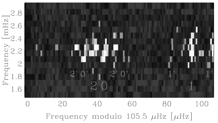
Figure 4: Echelle diagram of $\alpha$ Cen A oscillations. Modes $l$ = 0, 1 and 2 and their aliases are identified.

Fig. 5 corresponds to the merged echelle diagram, all the slices of 105.5 $\mu$Hz were summed up.

Both Figs. 4 and 5 make it possible to identify modes of degree $l$=0, 1 and 2 and their side-lobes due to the daily aliases at $\pm$ 11.57 $\mu$Hz. These two figures indicate that the modes follow an asymptotic relation reasonably well.

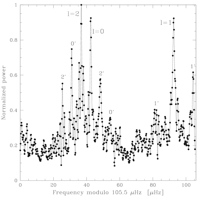
Figure 5: Sum of the echelle diagram of $\alpha$ Cen A oscillations. Modes $l$ = 0, 1 and 2 and their aliases are identified.

3.4 Gap filling process

In order to reduce the effect of single-site observation, the repetitive music process proposed by Fossat et al. (fossat99 (1999)) was used. This method is based on the fact that the autocorrelation function of the full disk helioseismological signal, after dropping quickly to zero in 20 or 30 minutes, shows secondary quasi periodic bumps, due to the quasi-periodicity of the peak distribution in the Fourier spectrum. In the helioseismological signal, the first of these bumps appears at about 4.1 hours and corresponds to a $\Delta\nu_{0}/2$ = 67.5 $\mu$Hz periodicity of the modes. An obvious consequence is that simply replacing a gap by the signal collected 4.1 hours earlier or 4.1 hours later provides a very efficient gap filling method. It should be noted that such a process modulates the background noise with the 67.5 $\mu$Hz periodicity, the fine adjustment of the method consists of placing the maxima of this modulation on the p-mode frequencies, so that any loss of information is located in the noise. This gap-filling process is not suitable if the modes do not follow an asymptotic relation. As precaution the frequency range should be cut in several parts and the fine tuning of the temporal periodicity adjusted in each of them.

In the case of $\alpha$ Cen A, the periodicity of the modes is equal to $\Delta\nu_{0}/2$ = 52.8 $\mu$Hz which correspond to a periodicity in time of the signal of about 5.26 hours. Considering that $\alpha$ Cen A was observed during the longest nights for a little less than 12 hours, this gap-filling process makes it possible to fill the duty cycle up to 90 %. The power spectrum of a pure sinusoid using the observational window of $\alpha$ Cen A with and without gap filling is presented in Fig. 6. Note that aliases at $\pm$ 1.35 $\mu$Hz are not reduced, due to the gap of the seventh and eighth nights during the run.

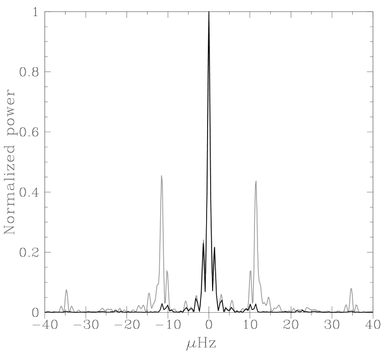
Figure 6: Observational window response with (black line) and without (grey line) the gap-filling process.

The frequency range was cut into 3 parts (1.8 - 2.2 mHz, 2.15 - 2.55 mHz and 2.5 - 2.9 mHz) and the temporal periodicity was adjusted in each of them to place the maxima of the modulation on modes $l$=1 which are easily identifiable. For the 3 parts of the power spectrum, the temporal periodicity used was respectively 5.299, 5.294 and 5.289 hours. The result is presented in Fig. 7.

This gap-filling process does not cause a drastic change in the power spectrum below 2.5 mHz. Above 2.5 mHz, the process helps in the identification of modes, especially modes $l$=0 and $l$=2 by removing or reducing aliases. Note that this process is based on the assumption that frequencies follow an asymptotic relation and can destroy any other frequency and/or enhance their side-lobes.

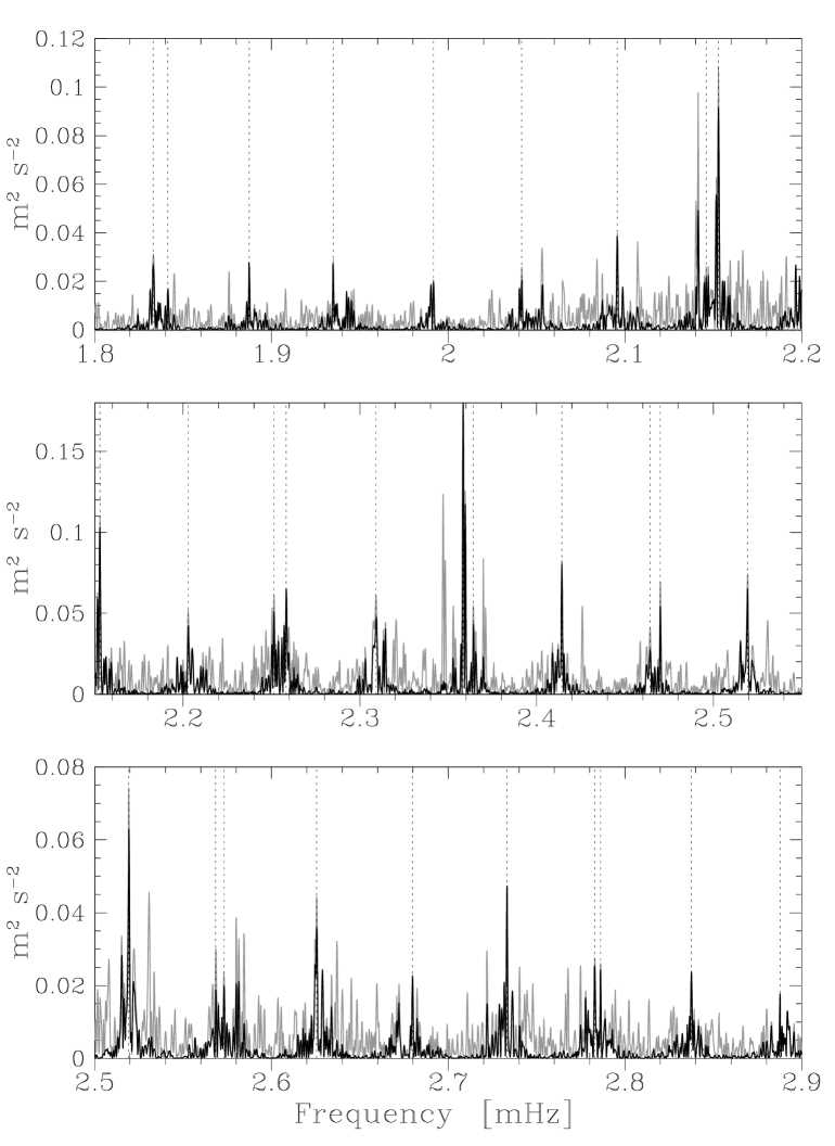
Figure 7: Power spectrum of $\alpha$ Cen A with (black line) and without (grey line) the gap filling process. The identified frequencies are indicated with dotted lines.

3.5 Frequencies of p-modes

The strongest peaks of the power spectrum computed with the gap filling process were identified and are listed in Table 2. These peaks were selected such as to have a signal-to-noise ratio in the amplitude spectrum greater than 3 (0.017  m² s^-2 in the power spectrum).

The frequency resolution of our time series is 0.93 $\mu$Hz. If we suppose that no mode is resolved, the estimated uncertainty on the frequency determination is 0.46 $\mu$Hz. The values of $n$ and $l$ are deduced from the asymptotic relation (see Eq. (1)) assuming that the parameter $\epsilon$ is near the solar value ($\epsilon_{\odot}\sim 1.5$). Our first identification in BC01 based on the 5 first nights did not make a distinction between the modes $l$=0 and $l$=2. The last row in Table 2 gives the average large spacing for each angular degree. All the identified modes in Table 2 are indicated in Fig. 7.

Table 2: Mode frequencies (in $\mu$Hz) of $\alpha$ Cen A. Uncertainty on frequency is estimated to 0.46 $\mu$Hz.

	$l$ = 0	$l$ = 1	$l$ = 2
n = 15			1833.1
n = 16	1841.3	1887.4	1934.9
n = 17		1991.7	2041.5
n = 18		2095.6	2146.0
n = 19	2152.9	2202.8	2251.4
n = 20	2258.4	2309.1	2358.4
n = 21	2364.2	2414.3	2464.1
n = 22	2470.0	2519.3	2568.5
n = 23	2573.1	2625.6
n = 24	2679.8	2733.2	2782.9
n = 25	2786.2	2837.6	2887.7
$\Delta\nu_{0}$	105.6 $\pm$ 0.5	105.6 $\pm$ 0.4	105.0 $\pm$ 0.5

The average large and small spacing and the parameter $\epsilon$ are deduced from a least-squares fit of Eq. (1) with the frequencies of Table 2:

$$\Delta\nu_{0}\,=\,105.5\,\pm\,0.1\;\mu Hz,$$

$$\delta\nu_{02}\,=\,5.6\,\pm\,0.7\;\mu Hz,$$

$$\epsilon\,=\,1.40\,\pm\,0.02\;.$$

Fig. 8 represents the echelle diagram of peaks listed in Table 2.

Figure 8: Echelle diagram of identified modes in the power spectrum. The modes $l$=2 ($\blacktriangle$), $l$=0 ($\square$) and $l$=1 ($\blacksquare$) are represented from left to right.

3.6 Amplitudes of p-modes

In order to estimate the average amplitude of the modes, we followed the method of Kjeldsen & Bedding (kjeldsen95 (1995)). A simulated time series was generated with artificial signal plus noise using our window function. The generated signal corresponds to modes centered on 2.36 mHz, separated by $\Delta\nu_{0}/2$ and convolved by a gaussian envelope. The generated noise is gaussian with a standard deviation of 1  m s^-1. Several simulations show that the envelope amplitude is in the range 29 - 33  cm s^-1.

Table 3 and Fig. 9 present the estimated Doppler amplitude of each identified mode with the assumption that none of them is resolved. This amplitude was determined as the height of the peak in the power spectrum after quadratic subtraction of the mean noise level. Fig. 9, like Fig. 5, shows that the modes $l$=0, 1 and 2 have a similar average amplitude.

Table 3: Doppler amplitude of identified modes determined as the height of the peak in the power spectrum after quadratic subtraction of the mean noise level.

$n$	$l$	$\nu_{n,l}$	An,l
		$\mu$Hz	cm s-1
15	2	1833.1	17
16	0	1841.3	12
16	1	1887.4	15
16	2	1934.9	16
17	1	1991.7	14
17	2	2041.5	15
18	1	2095.6	19
18	2	2146.0	15
19	0	2152.9	33
19	1	2202.8	22
19	2	2251.4	24
20	0	2258.4	25
20	1	2309.1	24
20	2	2358.4	44
21	0	2364.2	23
21	1	2414.3	28
21	2	2464.1	20
22	0	2470.0	26
22	1	2519.3	27
22	2	2568.5	17
23	0	2573.1	15
23	1	2625.6	21
24	0	2679.8	13
24	1	2733.2	21
24	2	2782.9	16
25	0	2786.2	15
25	1	2837.6	15
25	2	2887.7	12

Figure 9: Doppler amplitude of identified modes of degree $l$=0 ($\square$), $l$=1 ($\blacksquare$) and $l$=2 ($\blacktriangle$).

In order to compare the observed amplitude with the expected one, we computed the amplitude ratios between mode $l$=0 and the other modes $(l,m)$. These amplitude ratios (see Table 4) were determined following Gouttebroze & Toutain (goutte94 (1994)) assuming that all the modes have the same intrinsic amplitude. The effect of limb darkening was neglected and the inclination of the rotational axis was assumed equal to the inclination of the orbital axis of the binary system ($79^{o}$) determined by Pourbaix et al. (pourbaix99 (1999)).

Table 4: Expected amplitude ratios of modes.

$l$,$m$	amplitude ratios
$l$=0,$m$=0	1.00
$l$=1,$m$=0	0.25
$l$=1,$m$=-1,1	0.90
$l$=2,$m$=0	0.40
$l$=2,$m$=-1,1	0.21
$l$=2,$m$=-2,2	0.53
$l$=3,$m$=0	0.09
$l$=3,$m$=-1,1	0.12
$l$=3,$m$=-2,2	0.08
$l$=3,$m$=-3,3	0.18

The observed amplitude of modes $l$=2 is higher than expected; this can be due to interferences between modes of different $m$. The modes corresponding to $l$=3 are expected to have an amplitude of only 20 % of the $l$=1 mode, hence to be well below the threshold of identification.

3.7 Linewidth of p-modes and rotational splitting

The expected linewidth for a 1.1 M_⊙ star in the frequency range 1.8 to 2.9 mHz is less than 2 $\mu$Hz (Houdek houdek99 (1999)). Our frequency resolution of 0.93 $\mu$Hz is then too low to attempt a clear determination of the linewidth of the identified modes. Below 2.2 mHz, modes seem unresolved and present a linewidth equal to the frequency resolution, hence a damping time longer than 25 days. Above 2.2 mHz, the structure of modes seems more complex. This could be eventually caused by the fact that their linewidths begin to be greater than the frequency resolution.

For $\alpha$ Cen A, Hallam et al. (hallam91 (1991)) estimated a rotational period of 28.8 $\pm$ 2.5 days. More recently Saar & Osten (saar97 (1997)) measured a rotational velocity of 2.7 $\pm$ 0.7  km s^-1. With an estimated radius of 1.2 R_⊙, the period of rotation is 22 days. Assuming a uniform rotation, the corresponding splitting of the modes is expected to be about 0.5 $\mu$Hz. Assuming an inclination of the rotational axis of 79^o, a separation of about 1 $\mu$Hz should be visible between modes ($l$=1,$m$=-1) and ($l$=1,$m$=1), and modes ($l$=2,$m$=0) and ($l$=2,$m$=$\pm$2).

Figure 10: Superposition of identified modes $l$=0 ($\square$), $l$=1 ($\blacksquare$) and $l$=2 ($\blacktriangle$) in the power spectrum with frequency shifted to zero.

Figure 10 shows the superposition in the power spectrum of modes $l$=0, $l$=1 and $l$=2 with the frequency of each mode shifted to zero. Modes $l$=0 present side lobes at $\pm$ 1.35 $\mu$Hz, probably introduced by the aliases due to the gap of the seventh and eighth nights during the run. Modes $l$=2 present side lobes at $\pm$ 1.25 $\mu$Hz which could be introduced by these same aliases or/and a rotational splitting. In the latter case it should correspond to a period of rotation of about 19 days, lower than the expected one. Modes $l$=1, which show a side lobe only on the left, do not allow a conclusion. The CLEAN algorithm (Roberts et al. roberts87 (1987)) was used in order to remove the effect of the observational window response. We noticed that this process does not eliminate the whole signal at modes $l$=2, as is the case for $l$=0 and $l$=1. The pattern shown in Fig. 10 leads one to think that an error of $\pm$ 1.3 $\mu$Hz could have been introduced at some identified mode frequencies and could explain the dispersion of the mode frequencies around the asymptotic relation shown in Fig. 8.

Additional data will be needed to determine both the rotational splitting and the damping time of $\alpha$ Cen A p-modes.

4 Comparison with models

Seismological parameters deduced from our observations are in full agreement with the expected values scaling from the Sun (Kjeldsen & Bedding, kjeldsen95 (1995)) giving the frequency of the greatest mode $\nu_{\rm max}\,=\,2.3$ mHz, the large spacing $\Delta\nu_{\rm 0}\,=\,105.8$ $\mu$Hz and the oscillation peak amplitude $A_{\rm osc}\,=\,31.1$  cm s^-1.

The variations with frequency of the large and small spacings are compared in Figs. 11 and 12 with the values deduced from models recently developed by Morel et al. (morel00 (2000)) and Guenther & Demarque (guenther00 (2000)). The observational constraints for the model calibrations and the properties of the calibrated models are given in Table 5. The two sets of models differ essentially by the estimated mass and the age of the star. The large spacing, mainly related to stellar density, varies proportional to $M^{1/2}\,R^{-3/2}$. The small spacing, mainly related to the structure of the core, decreases with stellar age and mass.

Our observations are well bracketed by the two sets of models for both the large and small spacing. This clearly suggests a model with intermediate properties, i.e. a mass between 1.10 and 1.16 M_⊙. New models of $\alpha$ Cen A are being developed by Thevenin et al. (thevenin02 (2002)), with different properties in order to better interpret the observed oscillations and constraint the physical parameters of this star.

Table 5: Observational constraints and global characteristics of the models.

Models	Morel et al.	Guenther & Demarque
$M/M_{\odot}$	$1.16\pm 0.031$	$1.1015\pm 0.008$
$T_{\rm eff}[{\rm K}]$	$5790\pm 30$	$5770\pm 50$
$\log g$	$4.32\pm 0.05$	$4.28\pm 0.02$
$\rm[\frac{Fe}{H}]_{i}$	$0.20\pm 0.02$	$0.22\pm 0.02$
$L/L_{\odot}$	$1.534\pm 0.103$	$1.572\pm 0.135$
$t[{\rm Myr}]$	2710	5640
$Y_{\rm i}$	0.284	0.300
$(\frac{Z}{X})_{\rm i}$	0.0443	0.0480
$\alpha$	1.53	1.86

Figure 11: Variations of the large spacing between modes with consecutive radial order $\Delta\nu_{n,l}=\nu_{n,l}-\nu_{n-1,l}$ for p-modes of degree $l$=0 ($\square$), $l$=1 ($\blacksquare$) and $l$=2 ($\blacktriangle$) versus frequency. Upper lines correspond to the model of Morel et al. and lower lines to that of Guenther & Demarque. Solid, dashed and dotted lines correspond respectively to modes $l$=0, 1 and 2.

Figure 12: Variations of the small frequency spacing $\delta\nu_{02}=\nu_{n,0}-\nu_{n-1,2}$ versus frequency. The upper line corresponds to the model of Morel et al. and the lower line to that of Guenther & Demarque.

5 Conclusions and prospects

Our observations of $\alpha$ Cen A yield a clear detection of p-mode oscillations. Several identifiable modes appear in the power spectrum between 1.8 and 2.9 mHz with an average large spacing of 105.5 $\mu$Hz, an average small spacing of 5.6 $\mu$Hz and an envelope amplitude of about 31  cm s^-1. These characteristics, in full agreement with the expected values, make it possible to put constraints on the physical parameters of this star.

Additional data with a higher signal-to-noise and a higher frequency resolution will make it possible to determine properly the suspected rotational splitting and the damping time of $\alpha$ Cen A p-modes.

This result, obtained with a small telescope, demonstrates the power of Doppler ground-based asteroseismology. Future spectrographs like HARPS (Queloz et al. queloz01 (2001); Bouchy bouchy01 (2001)) are expected to conduct asteroseismological study on a large sample of solar-like stars, and to enlarge significantly our understanding of stellar physics.

- (1) Bedding, T. R., Butler, R. P., Kjeldsen, H., et al., 2001, ApJ, 549, L105
- (2) Bouchy, F., 2001, in : Radial and Nonradial Pulsations as Probes of Stellar Physics, IAU Coll. 185, C. Aerts, T.R. Bedding & J. Christensen-Dalsgaard (eds), ASP Conf. Ser., 256, 474
- (3) Bouchy, F., & Carrier, F., 2001, A&A, 374, L5
- (4) Brown, T. M., Gilliland, R. L., 1990, ApJ, 350, 839
- (5) Carrier, F., Bouchy, F., Kienzle, F., & Blecha, A., 2001a, in : Radial and Nonradial Pulsations as Probes of Stellar Physics, IAU Coll. 185, C. Aerts, T.R. Bedding & J. Christensen-Dalsgaard (eds), ASP Conf. Ser., 256, 468
- (6) Carrier, F., Bouchy, F., Kienzle, F., et al., 2001b, A&A, 378, 142.
- (7) Carrier, F., Bouchy, F., Provost, J., et al., 2001c, in : Radial and Nonradial Pulsations as Probes of Stellar Physics, IAU Coll. 185, C. Aerts, T.R. Bedding & J. Christensen-Dalsgaard (eds), ASP Conf. Ser., 256, 460
- (8) Edmonds, P. D., & Cram, L. E., 1995, MNRAS, 276, 1295
- (9) Fossat, E., Kholokov, Sh., Gelly, B., et al., 1999, A&A, 343, 608
- (10) Gelly, G., Grec, G., Fossat, E., 1986, A&A, 164, 383
- (11) Gouttebroze, P., & Toutain, T., 1994, A&A, 287, 535
- (12) Grec, G., Fossat, E., Pomerantz, M.A., 1983, Sol. Phys., 82, 55
- (13) Guenther, D. B., & Demarque, P., 2000, ApJ, 531, 503
- (14) Hallam, K.L., Altner, B., Endal, A.S., 1991, AJ, 372, 610
- (15) Houdek, G., Balmforth, N.J., Christensen-Dalsgaard, J., et al., 1999, A&A, 351, 582
- (16) Kjeldsen, H., & Bedding, T. R., 1995, A&A, 293, 87
- (17) Kjeldsen, H., Bedding, T. R., Frandsen, S., et al., 1999, MNRAS, 303, 579
- (18) Leighton, R.B., Noyes, R.W., & Simon, G.W., 1962, ApJ, 135, 474
- (19) Lomb, N. R., 1976, Astrophys. & Space Sci, 39, 447
- (20) Martic, M., Schmitt, J., Lebrun, J.-C., et al., 1999, A&A, 351, 993
- (21) Morel, P., Provost, J., Lebreton, Y., et al., 2000, A&A, 363, 675
- (22) Pottasch, E. M., Butcher, H. R., van Hoesel, F. H. J., 1992, A&A, 264, 138
- (23) Pourbaix, D., Neuforge-Verheecke, C., & Noels, A., 1999, A&A, 344, 172
- (24) Thevenin, F., et al., 2002, A&A, submitted
- (25) Queloz, D., Mayor, M., et al., 2001, The Messenger, 105, 1
- (26) Roberts, D. H., Lehar, J., & Dreher, J. W., 1987, AJ, 93, 968
- (27) Saar, S.H., Osten, R.A., 1997, MNRAS, 284, 803
- (28) Scargle, J. D., 1982, ApJ, 263, 835
- (29) Schou, J., & Buzasi, D. L., 2001, Proc. SOHO 10/GONG 2000 Workshop, ”Helio- and Asteroseismology at the Dawn of the Millennium”, Tenerife, Spain (ESA SP-464)
- (30) Tassoul, M., 1980, AJS, 43, 469
- (31) Ulrich, R.K., 1970, ApJ, 162, 993