The Detectability of Neutralino Clumps via Atmospheric Cherenkov Telescopes
Abstract
High resolution N-body simulations have revealed the survival of considerable substructure within galactic halos. Assuming that the predicted dark matter clumps are composed of annihilating neutralinos, we examine their detectability via Atmospheric Cherenkov Telescopes (ACTs). Depending on their density profile, individual neutralino clumps should be observable via their -ray continuum and line emissions. We find that the continuum signal is the most promising signal for detecting a neutralino clump, being significantly stronger than the monochromatic signals. Limits from the line detectability can help lift degeneracies in the supersymmetric (SUSY) parameter space. We show that by combining the observations of different mass clumps, ACTs can explore most of the SUSY parameter space. ACTs can play a complementary role to accelerator and -ray satellite limits by exploring relatively large neutralino masses and less concentrated clumps. We develop a strategy for dark matter clump studies by future ACTs based on VERITAS specifications and encourage the development of techniques to identify primaries. This can reduce the background by an order of magnitude.
pacs:
95.35.+d; 98.35GiI Introduction
The presence of a dark matter component is inferred through gravitational interactions in galaxies and clusters of galaxies. Its contribution is estimated to be about 30% of the critical density of the Universe. This dark matter cannot be all baryonic. Constraints from primordial nucleosynthesis and cosmic background radiation measurements limit the baryonic content of the Universe to be at most about 4% of the critical density. The remaining 26% of the critical density is believed to be composed of a, yet to be observed, Cold Dark Matter (CDM) particle.
Among the several candidates proposed for the non-baryonic dark matter, the leading scenario involves Weakly Interacting Massive Particles (WIMPs). Weakly interacting relics from the early universe with masses from some tens of GeV to some TeV can naturally give rise to relic densities in the range of the observed dark matter density. WIMPs are also well motivated by theoretical extensions of the standard model of particle physics. In particular, the lightest supersymmetric particle (LSP) in supersymmetric extensions of the standard model can be a WIMP that is stable due to R-parity conservation. In most scenarios the LSP is neutral and is called the neutralino, (for a review see, e.g., jkg96 ).
Neutralinos may be detected directly as they traverse the Earth, may be generated in future particle colliders, and may be detected indirectly by observing their annihilation products. Direct neutralino searches are now underway in a number of low background experiments with no consensus detection to date. Collider experiments have been able to place some constraints on the neutralino parameter space (see, e.g., efgo00 ), but a large region of the parameter space is still unexplored. Indirect searches offer a viable and complementary alternative to direct searches and accelerator experiments. In particular, neutralino annihilation in the galactic halo can be observed via -rays, neutrinos, and synchrotron emission from the charged annihilation products bgz92 ; bbm94 ; gs99 ; bss01 ; g00 ; begu99 ; cm01 ; abo02 ; bot02 ; t02 .
The rate of neutralino annihilation is proportional to the neutralino number density squared (), thus the strongest signals are likely to come from either the galactic center bgz92 ; bbm94 ; gs99 ; bss01 ; g00 ; begu99 , or the higher density nearby clumps of dark matter in our halo begu99 ; cm01 ; bot02 ; abo02 . The dark matter density in the galactic center depends strongly on the formation history of the central black hole mm02 , and its -ray emission due to neutralino annihilation may be difficult to distinguish from other baryonic -ray sources. As an alternative, the clumpy nature of CDM halos provides a number of high density regions, other than the galactic center.
Clumps of dark matter distributed throughout galaxy halos is a generic prediction of high-resolution CDM simulations (see, e.g., gmglqs ; Moore1 ; Klypin1 ; iro02 ). This high degree of substructure is what has remained from the merging of small halos to form the larger halos (either cluster or galaxy halos). Simulations show that about to of the total mass of a given halo is in the form of smaller mass clumps. These clumps are ideal sites for neutralino annihilation and can be observed via their -ray signal begu99 ; cm01 ; abo02 , and via their synchrotron emission bot02 . Here, we study in detail the -ray emission from the nearest clumps of dark matter via Atmospheric Cherenkov Telescopes (ACTs), such as VERITAS veritas , HESS hess , MAGIC magic , and CANGAROO-III cang3 . We explore the neutralino parameter space for the continuum, the , and the lines and calculate the flux of different mass clumps assuming different clump density profiles and VERITAS specifications. We find that the larger mass clumps can be easily detected by the next generation ACTs and that the detectability of the smaller mass clumps can help constrain the neutralino parameter space. Future ACT observations are only limited by their threshold energy and will be more effective for neutralino masses above 50 to 100 GeV, a range of neutralino masses that nicely complements accelerator and satellite studies of the neutralino parameter space.
In the next section, we discuss the structure and the mass spectrum of the dark matter clumps that we assume in our study. In §III, we present the neutralino parameter space for continuum -rays, the , and the line emission using DarkSUSY darksusy1 . In §IV, we discuss the characteristics of ACTs and the relevant backgrounds. Our results and strategies for CDM clump detection are shown in §V. Finally, we conclude in §VI.
II The dark matter clumps
II.1 The nearest clumps
According to N-body simulations gmglqs ; Moore1 ; Klypin1 , substructures of masses survive in significant numbers in galactic halos. Within the virial radius of a galactic halo about 10%-15% of the mass is in the form of dark matter clumps. The mass spectrum for the simulated dark matter clumps in galactic halos is of the form (e.g., Moore1 ; Klypin1 )
| (1) |
for clumps with mass , the lowest resolvable mass, approximately. Clumps are more numerous the less massive they are, thus one would expect a large number of relatively light clumps. Simulations find (e.g., Moore1 ). We adopt the same value here and extrapolate to lower masses than those presently resolved by simulations. With this extrapolation we can estimate the numbers of clumps in specific mass bins, as well as the distances to the nearest of these clumps.
In order to find the proportionality constant in Eq.(1), we normalize the mass function so that 500 satellites exist within the galactic halo with masses above , in agreement with the predictions of N-body simulations for a halo like ours Moore1 . Thus we find for the predicted number, , of clumps with mass greater than , in solar masses,
| (2) |
where is the maximum mass clump in the halo. Using our halo as the host within which the clumps are orbiting, we assume .
The number, , of clumps predicted in several mass bins that lie in the mass range from up to are tabulated in the first and second columns of Table 1. We choose each bin labeled by to contain clumps with mass in the range , and calculate . The numbers appear to be high enough, and even though they are consistent with simulations, the question whether they can be realistic is raised. Contrary to what was initially believed, namely that large numbers of substructures within a galactic halo might threaten the stability of the disk, nowadays we know that this is not the case (for a recent review, see iro02 ). It has been found, first, that the orbits of satellite substructures in present-day halos very rarely take them near the disk font , and second, that disk overheating and stability would become real problems only when interactions with numerous, large satellites (e.g., the LMC) take place waketal ; veletal . Consequently, these numbers can be considered perfectly realistic. In the third column of Table 1 we give values of the mean inter-clump distance in a specific mass bin, assuming that the clumps are homogeneously distributed within the virial extend of the halo. Thus, in the third column we have the quantity , with the virial radius of the galactic halo which we take to be equal to 300 kpc. However, clumps are unlikely to be homogeneously distributed in the host halo. It is believed that they are distributed in a way similar to the way the smooth component of the dark matter halo is distributed (e.g., Pasquale1 ). Thus, we estimate another measure for the distance, the distance to the nearest clump for each mass bin, as follows: first, we calculate the fraction, , of the total dark matter of the galaxy which is in the form of clumps of mass and take . For a local dark matter density pc3 and using the above fractions we find the local dark matter density which is in clumps of a specific mass. Going from the mass to the number density, we find the distance to the nearest clump, (see also Lake1 ; Bergstrom2 ). As we can see from Table 1, can be a factor of ten smaller than the mean distance as calculated in the homogeneous distribution case. We use below when estimating -ray fluxes from different clumps.
| (pc) | (pc) | ||
|---|---|---|---|
| 504 | 61 | ||
| 1014 | 123 | ||
| 2037 | 246 | ||
| 4050 | 490 | ||
| 8040 | 973 | ||
| 16023 | 1939 | ||
| 32013 | 3874 |
One should keep in mind that since we only have one halo to probe, our galactic halo, the actual distances to the nearest clumps will have large fluctuations. For a number of realizations of the clumpy halo in -rays, see abo02 . Instead of simulating the sky, we focus on the strategy for future ACT studies based on . As will be shown, the results we derive can be easily extended to accommodate different clump distances from the ones we use. A deeper understanding of the clump space distribution awaits higher resolution simulations.
II.2 The structure of the dark matter clumps
We model the clumps using three different mass density profiles, , the Singular Isothermal Sphere (SIS), the Moore et al. Moore1 , and the Navarro, Frenk and White (NFW) navarro1 density profile. The SIS profile is described by
| (3) |
and represents a reasonable upper limit to the degree of central concentration of the clumps. At the center, the SIS density profile diverges as . The Moore et al. density profile is given by
| (4) |
where and are the characteristic density and scale radius of the configuration, respectively. This profile is the one suggested by numerous N-body simulations and is used in our study as representative of the intermediate concentration cases, at least compared to the other two density profiles. It is divergent at the center where it behaves as , whereas at large distances () it behaves as . The NFW profile navarro1 can be written as
| (5) |
This profile was the first proposed density profile for the dark matter halos produced in simulations. It is divergent at the center with an behavior, namely it is shallower, less centrally concentrated than both the SIS and the Moore et al. profiles. At larger radii, NFW behaves as , exactly the same way as the Moore et al. profile. Note that the two quantities, and , in the NFW and Moore et al. profiles are not the same for the same clump (for a comparison, see klypin ). We choose to use the NFW profile as the least centrally concentrated density profile. The density profile derived from Taylor and Navarro (TN)taylor ; taynav , which is even shallower at the center behaving as , is a possibility; it will give lower fluxes than the cuspier NFW, with the latter, as will be seen in what follows, being difficult to detect. The TN will be even more difficult to detect, implying for its detectability neutralino annihilation cross sections higher than the relevant range of values as predicted by supersymmetric models.
Our final three choices represent well a range of possible concentrations of clumps in the galactic halo. In reality, the SIS configuration is very hard to achieve dynamically and has been recently ruled out for most of the clumps in our halo by EGRET bounds abo02 . We consider the SIS case to illustrate the range of clumps more highly concentrated than Moore et al. In addition, individual clumps may vary in concentration, given a range of possible initial conditions for a dark matter overdensity. Thus, an individual clump may be more highly concentrated than the mean. A possible range in concentrations should be kept in mind in general searches such as the one we study here.
For a specific clump mass and distance, we need to determine the parameters of each of the three profiles. In the case of the SIS, we use the following two conditions to calculate and the radius of the clump, :
-
1.
The volume integral of the density must yield the mass of the clump:
(6) -
2.
The density of the clump at distance from its center must equal the local density, , of the galactic (host) halo at distance , with the distance of the clump from the center of the host halo:
(7)
For the case of either the Moore et al. or the NFW density profile, we use Eqs.(6) and (7), but we need a third equation since we have three unknown quantities , , and . The third condition comes from the requirement that the radius of the clump be (smaller or) equal to the tidal radius (see, e.g., binney ). This guarantees that the clump is not tidally stripped. Thus,
| (8) |
with the galactic halo mass inside a sphere of radius . The SIS configuration is also stable against tidal stripping, as can be seen by considering the similar meaning of Eqs.(7) and (8).
In both Eqs.(7) and (8) we need to specify the density profile of the galactic halo. Both the Moore et al. and the NFW profile are acceptable profiles for its description. Furthermore, for our purposes, they are essentially equivalent descriptions. Convergence studies have shown that these two density profiles are very similar at radii above of the virial radius (e.g., klypin ). For a virial radius for our halo 300 kpc, this means that the two density profiles are different only within the inner 3 kpc. Given that we are at 8.5 kpc from the galactic center, and given the nearest clump distances presented in Table 1, the relevant distances from the center of the halo we are concerned with are far larger than 3kpc; thus, it is not of crucial importance whether the NFW or the Moore et al. density profile is used for the galactic halo one . We choose the NFW profile to model the galactic halo, regardless of the density profile assumed for the clumps. For we use 27.7 kpc to match simulation results cm01 . To find , the characteristic density for our galaxy, we normalize the density profile so that the peak circular velocity is about 220 km/sec, and thus
| (9) |
with , and = 8.5 kpc our galactocentric distance. Finally,
| (10) |
One final characteristic of the dark matter clump structure is the core radius. Inside some radius , the annihilation rate becomes so large that the overdensity is destroyed as fast as it can fill the region, yielding thus a constant density core. Following bgz92 , we find by equating the annihilation time scale to the free-fall time scale,
| (11) |
In this way we derive a maximum possible . The actual value might be smaller. Note that the choice of affects only the results for the SIS density profile since, as can be easily verified for the simple case of an unresolved clump, the flux coming from such a clump scales as (see section IV). In the case of the Moore et al. density profile the -dependence of the flux is via the factor , approximately, with and . Namely, the Moore et al. conclusions are not sensitive to the exact choice of comment . In the case of the core-dominated fluxes of an SIS clump, using the maximum will yield the minimum fluxes. As will become clear from our results however, the conclusions do not change, at least qualitatively, since the SIS is steep enough to be detectable even when using these minimum fluxes.
Below we discuss the annihilation cross sections into either continuum or monochromatic -rays. We find that the dominant cross section times relative velocity product corresponds to annihilation into the continuum, , and even though, in principle, all annihilation channels contribute in smearing out the central cusp, we use this dominant cross section in Eq.(11) to find .
III Neutralino annihilation as a gamma-ray source
III.1 The Neutralino-Supersymmetric models for dark matter
Following Bergstrom2 ; Baltz1 ; Bergstrom3 ; Edsjo1 , we work in the frame of the Minimal Supersymmetric extension of the Standard Model (MSSM) using the computer code DarkSUSY darksusy1 . The general R-parity conserving version of this model is characterized by more than a hundred free parameters. It is of common praxis to make some simplifying assumptions which leave only 7 parameters, the higgsino mass parameter , the gaugino mass parameter , the ratio of the Higgs vacuum expectation values given by , the mass of the CP-odd Higgs boson , the scalar mass parameter , and the trilinear soft SUSY-breaking parameters and for third generation quarks (for a discussion of the model and the simplification procedure, the results of which DarkSUSY incorporates, see Bergstrom4 ; Bergstrom8 ; Bergstrom9 ).
The LSP in most models is the lightest of the neutralinos. Neutralinos are a linear superposition of four neutral spin- Majorana particles: the superpartners of the Higgs, namely the neutral, CP-even higgsinos and , and the superpartners of the electroweak gauge bosons, namely the bino and the wino . After electroweak symmetry breaking, these gauge eigenstates mix. The diagonalization of the corresponding tree-level mass matrix gives the neutralinos,
The lightest of these, the , is assumed to be the LSP and is referred to as the neutralino. Due to R-parity conservation the neutralino is stable, since there is no allowed state for it to decay into. Its mass is somewhere between some tens of GeV up to several TeV. It is cold, namely non-relativistic when decoupled, and is considered one of the most plausible candidates for the CDM particle.
Using DarkSUSY, we made random scans of the parameter space, with overall limits for the seven MSSM parameters as given in Table 2. For the neutralino and chargino masses, one-loop corrections were used in accordance to hfast1 , whereas for the Higgs bosons the leading log two-loop radiative corrections were calculated using the code FeynHiggsFast hfast incorporated in DarkSUSY.
| Parameter | |||||||
|---|---|---|---|---|---|---|---|
| unit | GeV | GeV | 1 | GeV | GeV | 1 | 1 |
| Min | 3.0 | 0 | 100 | ||||
| Max | 60.0 | 10000 | 30000 |
We scanned the parameter space to obtain the boundaries of the allowed SUSY parameter space which we plot in FIGs.1-3, 5, and 7. For each model, we checked whether it is excluded by accelerator constraints. We used the latest constraints available in the DarkSUSY package, namely the 2000 constraints which are adequate for our purposes. The most important constraints come from the LEP collider at CERN, with respect to the lightest chargino and the lightest Higgs boson mass, as well as constraints from (for more details see, e.g., Baltz1 and references therein). For each model consistent with the accelerator constraints, we calculated the corresponding , with the neutralino relic density in units of the critical density, and the Hubble parameter today in units of 100 km s-1 Mpc-1. DarkSUSY calculates the relic density solving the Boltzmann equation numerically, while taking into account resonances and thresholds, and all the tree-level 2-body annihilation channels (see, Edsjo1 ; Gondolo1 ). We take into account the coannihilations between the lightest neutralino and the heavier neutralinos/charginos only if the mass difference is less than , obtaining thus a relic density with accuracy , which is reasonable for our purposes. Lastly we are interested in models in which the corresponding relic abundance contributes a significant, but not excessive amount to the overall density. We choose the range
| (12) |
to be consistent with cosmological constraints. The lower limit in inequality (12) is chosen on the basis that for values lower than 0.1 there is not enough dark matter to play a significant role in structure formation, or to constitute a large fraction of the critical density. The upper bound is chosen on the basis that, given that there is a minimum age for the Universe, there is a maximum value that the dark matter density can have. The upper limit 0.3 corresponds to a minimum age of 12 Gyr approximately (see, e.g., Peacock1 ). Note that the choice of for the upper limit can be considered generous, especially given the results from recent SN observations reiss1 ; Perlmutter1 , which constrain the allowed relic density to about , with .
III.2 Gamma-rays from neutralino annihilation
Neutralinos annihilate through a variety of channels. We will focus on the continuum -rays, and on the two monochromatic lines that are produced through the cascade decays of other primary annihilation products. The continuum contribution is mainly due to the decay of mesons produced in jets from neutralino annihilations. Schematically,
| (13) | |||||
To model the fragmentation process and extract information on the number and energy spectrum of the -rays produced, we adopt a simplified version of the Hill spectrum hill1 ; hill2 for the total hadron spectrum produced by quark fragmentation based on the leading-log approximation (LLA),
| (14) |
where , and is the energy of a hadron in a jet with total energy equal to the neutralino mass, . Assuming that all the hadrons produced are pions, which is very close to reality, and assuming that each pion family takes approximately of the total pion content of each jet we may write for the spectrum,
| (15) |
with . Furthermore, the probability per unit energy that a neutral pion with energy produces a photon with energy through the process shown in Eq.(13) is . Thus, from Eq.(15) we get for the continuum photon spectrum,
| (16) |
with and .
The continuum signal lacks distinctive features; this might make it difficult to discriminate from other possible -ray sources. A more unique signature is given by monochromatic -rays, which arise from loop-induced s-wave annihilations into the and the final states. These lines are free of astrophysical backgrounds. The respective spectra for the two lines are:
-
•
For the , 2 photons at
-
•
For the , 1 photon at ,
as can be easily verified by the conservation laws and the fact that the neutralinos are expected to be highly non-relativistic.
Note that for high values, the energies of the two lines are expected to coincide. Furthermore, in the case of the line, the energy of the photon becomes vanishingly small as tends to . Below , the process is no longer kinematically allowed.
IV The gamma-ray signal
IV.1 Fluxes and counts
We derive the fluxes for resolved and unresolved clumps as a function of the neutralino parameters, and the size and distance of the clumps, assuming the nearest clump for each mass bin. To turn the estimated fluxes into photon counts collected by an ACT, we need to specify the characteristics of the particular ACT. We choose to use VERITAS as the standard next generation ACT and list its specifications in Table 3.
| Energy range | 50 GeV-50 TeV | |
|---|---|---|
| Energy resolution | ||
| Effective area | Angular resolution | |
| cm2 | at 100 GeV | |
| cm2 | at 300 GeV | |
| cm2 | at 1 TeV |
The number, , of annihilations per unit volume and time is
| (17) |
where is the number density of neutralinos, and is the thermally averaged product of the cross section times the relative velocity two for the continuum -rays (=cont.), the 2 line (=), and the line (). Denoting by the number of -rays emitted per annihilation, with energy above the energy threshold used, then (provided that ), and (provided that ); can be obtained by integrating the spectrum given by Eq.(16),
| (18) |
where .
The emission coefficient , namely the number of emitted photons per unit time and volume, will be
| (19) |
where is the mass density of neutralinos.
Given the expression for the emission coefficient, we can calculate the flux coming from a clump. The observed flux at the Earth depends on whether the object is resolved or unresolved by the ACT, namely, whether the angular size of the clump is larger or smaller than the angular resolution of the instrument. More specifically, in the case where the clump under consideration is unresolved, its flux at the Earth, , is given by the volume integral of the emission coefficient divided by the area ,
| (20) |
where denotes the distance of the clump from the Earth and is, as before, the clump radius. At this point, note that and (appearing in Eqs.(7) and (8)) are two different quantities; is the distance of the clump from the Earth, whereas is the distance of the clump from the center of the Milky Way. For a clump with galactic coordinates (,), the two quantities are related via the expression,
| (21) |
with 8.5 kpc. If the clumps are resolved, the corresponding flux at the Earth, , is given by the integral along the line of sight of the emission coefficient,
| (22) |
In the case of the unresolved sources, the source counts, , will be simply,
| (23) |
with the effective collecting area of the instrument and the integration time. For a resolved clump, we can define its surface brightness as seen by an ACT as
| (24) |
where and the same as above. To obtain the number of photons, , that the instrument will collect from the source, assuming that we observe the central pixel, we integrate the surface brightness of the source over a disk centered on the source with angular radius equal to the angular resolution of the instrument ,
| (25) |
The angular resolution of the instrument defines a maximum projected size for a clump at distance by . Similarly, . Substituting Eqs.(22) and (24) in Eq.(25) we obtain,
| (26) |
IV.2 Background counts
The detectability of the clumps depends on their fluxes as compared to the possible background contributions. As we discuss below, the dominant background contributions are due to electronic and hadronic cosmic ray showers. Efforts to discriminate between photon primaries versus charged primaries can help improve considerably the detectability of dark matter clumps. We also discuss the galactic and extragalactic -ray backgrounds, as well as the contribution from the rest of the dark matter halo component.
IV.2.1 Electronic and hadronic cosmic ray showers.
For the background rate of -like hadronic showers we use the integral spectrum presented in Bergstrom6 ,
| (27) |
This was derived from data taken with the Whipple 10m telescope. VERITAS is expected to have an improved method for rejecting charged primary showers, compared to the Whipple telescope. However, aiming at a conservative treatment, we do not take this into account. For the electron-induced background we use the following integrated spectrum Longair ,
| (28) |
The electron-induced showers at Whipple are indistinguishable from -rays and can be rejected only on the basis of their arrival direction, whereas the hadron-induced showers are more extended on the ground than the electron-induced ones. Furthermore, we see that cosmic-ray electrons have a steeper spectrum than cosmic-ray nuclei and dominate the background at low energies.
IV.2.2 Extragalactic and galactic -ray emission.
For the extragalactic diffuse emission, we use a fit to the EGRET data, valid for the energy range from 30 MeV to 100 GeV Sreekumar
| (29) |
The galactic diffuse emission is thought to be mainly due to cosmic-ray protons and electrons interacting with the interstellar medium. It is enhanced towards the galactic center and the galactic disk, and has been measured by EGRET Sreekumar ; Hunter up to about 10 GeV. For its differential spectrum we use the expression provided in Bergstrom6 , namely a power law fall-off in energy of the form
| (30) |
The factor depends only on the galactic coordinates and has been fixed using EGRET data at 1 GeV (see Bergstrom6 , and references therein). It is given by
| (31) | |||||
with and varying in and , respectively. This expression is in reasonable agreement with data especially towards the galactic center. The exponent in principle depends on both the energy range and the galactic coordinates; as in Bergstrom6 ; Bergstrom7 , we use , assuming the behavior continues at higher energies.
It is also important to obtain an estimate of the -ray counts due to neutralino annihilation in the smooth dark matter component of the galactic halo. The flux of continuum -rays of the smooth halo component is given by
| (32) |
with given by Eq.(10), and the angle of the direction of observation with respect to the direction of the galactic center. This flux is clearly enhanced towards the central regions of the galaxy (for more details see, e.g., cm01 ). In order to estimate a value close to the maximum possible smooth component counts, , we use the direction – close to the center. The flux coming from this direction is approximately
| (33) |
The emission due to the total clumped component of the dark matter halo, as seen in cm01 ; abo02 , overwhelms the smooth component -ray emission. Note that neither the smooth, nor the clumped component -ray emission constitutes an additional background for our study. For example, part or all of the extragalactic background, which we have already taken into account, would be due to numerous, unresolved clumps in our halo. In fact, this has allowed ref. abo02 to place strong limits on the neutralino parameter space for clumped halos with SIS and Moore et al. clump profiles, by comparing the clumped component -ray emission with the extragalactic diffuse -ray emission (Eq.(29)). In particular, an SIS clump distribution would surpass EGRET bounds for all of the SUSY models usually considered for neutralinos.
In order to estimate the relative importance of the several contributions we assume an ACT observation with the following characteristics: cm2, hrs, GeV, . For these parameters, we find the counts , , , (for GeV and, referring to the continuum -rays, for a typical cross section we obtain , rounding off to the closest integer). To calculate the galactic background counts, we made the conservative assumption of the maximum possible background and, thus, used . This background is anisotropic and will be lower at higher galactic latitudes. Evidently, the main backgrounds for ACT searches are the hadronic and electronic backgrounds. Only if the composition of primaries can be identified, the galactic and the extragalactic diffuse -ray backgrounds become important; this would be highly desirable, given that the galactic background is (at least) an order of magnitude lower than the cosmic ray induced backgrounds.
We chose to keep a conservative estimate of the backgrounds by considering the two dominant backgrounds, the electronic and the hadronic cosmic-ray induced ones, since, as we have shown above, the other contributions are at least one order of magnitude lower. Thus, the background counts in the case of the continuum are
| (34) |
where we define as the sum of the hadronic and the electronic cosmic ray induced backgrounds, as given by Eq.(27) and (28), respectively. In the case of the lines the background counts are given by
| (35) |
where stands for the energy of the line and stand for and respectively, with denoting the energy resolution of the detector.
Note that the only anisotropic background – the galactic – is negligible in comparison with the charged particle backgrounds. This makes our calculations essentially independent of the exact direction of the clump in the sky. Any particular choice of galactic coordinates would not limit the generality of our conclusions with respect to the observability of the clumps. The only assumption we should make is that the clumps are more likely to be found away from the galactic plane. This is to be expected since simulations show that the orbits of CDM satellites in present-day halos very rarely take them near the disk (e.g., font ). This is not a very constraining assumption – all directions in the sky that avoid the galactic disk are essentially equivalent – and thus, the only really important quantity with respect to the location of a clump is its distance from us. The exact galactic coordinates can in principle be important via Eqs.(7) and (21), but it turns out that this is not the case. For example, considering the clumps with mass and nearest distance of about kpc (see Table 1), we find that putting such a clump towards the galactic center yields kpc-3, whereas putting it in the exact opposite direction, towards the anticenter, yields kpc-3, namely there is no significant variation.
V Results
V.1 The detectability condition
The background follows Poisson statistics and as such it exhibits fluctuations of amplitude . For given technical and observation parameters, the minimum detectable flux of -rays for an ACT is determined by the condition that the significance exceeds a specific number, , of standard deviations, , or that the number of detected photons exceeds a specific number . Namely,
| (36) |
and,
| (37) |
The first condition simply defines what achieving an - detection requires. The second condition ensures that we obtain sufficient statistics of -ray events and is useful especially at the higher energies ( TeV), where the backgrounds are negligible, and thus the first condition is useless. The second condition also shows that at high energies, whether the source will be detectable or not is determined only from its high energy spectrum (and the ACT characteristics). Given that we start at tens of GeV energy thresholds, we check for the first condition making sure that the second condition is satisfied as well. We require a 5- detection level (). As has been already mentioned, for all the mass bins studied, the nearest clump can be resolved for standard ACT angular resolutions (see Table 3), and thus we use Eq.(26) for , whereas for the background we use either Eq.(34) or Eq.(35), depending on whether we study the continuum or the lines, respectively.
Using the aforementioned detectability condition, we can constrain the SUSY parameter space. In addition to the unknown neutralino parameters, and , we do not know the precise density profiles of the dark matter clumps. In the figures that will follow, we take under consideration the profile uncertainties by using the three density profiles mentioned before (the SIS, Moore et al., and NFW profiles). We then set the constraints on the neutralino parameter space as follows: we substitute Eq.(26) for , and Eq.(34) or (35) for , as well as the expressions for in condition (36), and then we solve the resulting inequality with respect to . This yields an inequality of the form
| (38) |
In other words, an - detection for given , , , , , and can be obtained as long as is above a certain value which depends on and the integral of the density squared, which we have denoted by . Thus, plotting inequality (38) with the equality sign onto the SUSY parameter space, we divide the SUSY parameter space into the detectable (above the line defined by (38)) and the undetectable (below the line defined by (38)) regions.
In another set of figures, we show the flux for a given clump as a function of , assuming a typical value, , for the cross-section. This is interesting to be compared to the dominating backgrounds, as well as to what we call the minimum detectable flux , which we define using again the detectability criterion given in (36). More specifically, for the minimum required source counts , so that an - detection level be achieved we will have from (36)
| (39) |
For we obtain,
| (40) |
This is separately applicable for the continuum and the lines.
V.2 Continuum -rays
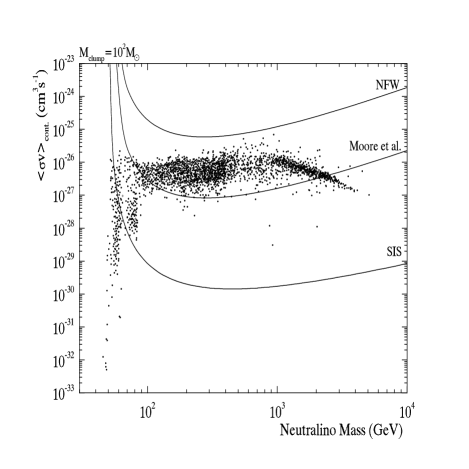
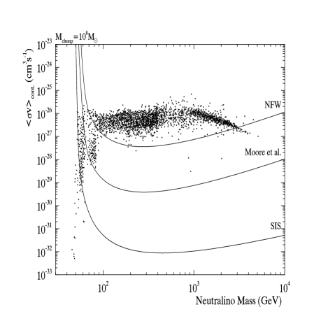
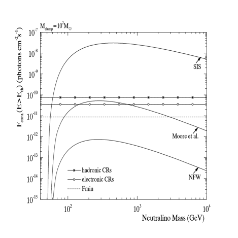
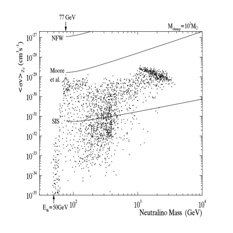
The minimum detectable neutralino annihilation cross section into continuum -rays as a function of neutralino mass for a and a dark matter clump is shown in FIG.1. These curves were obtained using condition (38) for cm2, s (100 hrs), GeV and (these are also the parameters we use for the rest of the figures, unless otherwise stated). In the same figure, the three cases of clump modeling using an NFW, a Moore et al., or an SIS density profile are shown. Note that by plotting the results for the minimum and the maximum clump masses that we considered, and , respectively, any other clump mass choice lies in between. The same is true for the density profiles, at least with respect to the degree of central concentration: any profile steeper than the NFW and softer than the SIS will be a curve between the two limiting curves defined for a specific clump mass, by the SIS and the NFW profiles, and as an example we plot the Moore et al. case.
In the case of a clump, we see that if the clump were described by a density profile as centrally concentrated as the SIS, then it would be detectable for most neutralino parameters, unless 70 GeV. The same clump modeled with the Moore et al. profile has good chances to be detected, since for a large range of the curve is below most of the possible models. Furthermore, note that given the recent results from abo02 , these highly centrally concentrated clumps would have to be a rare event among concentrations of halo clumps.
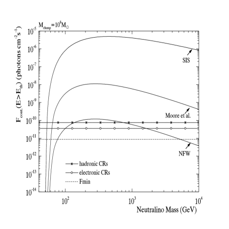
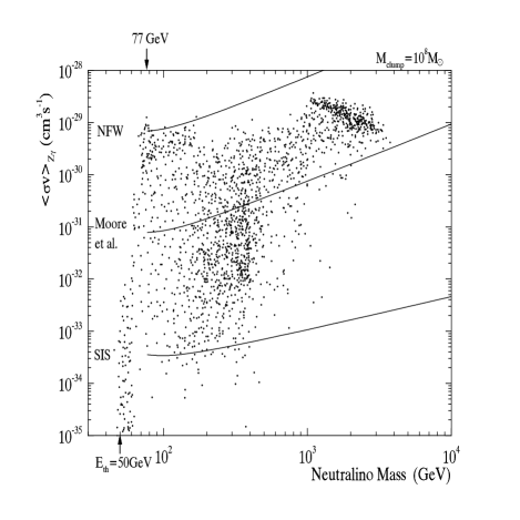
The same results are plotted for a clump with mass . The minimum detectable for all the three profiles goes down by approximately two orders of magnitude, compared to the case. As a result, such a massive clump is most likely detectable, even if it is best described by the least concentrated density profile, the NFW. Note also that, referring to the low mass clumps, the NFW case is, compared to the other density profiles, the most consistent profile with EGRET bounds abo02 .
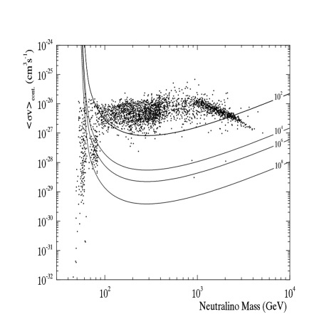
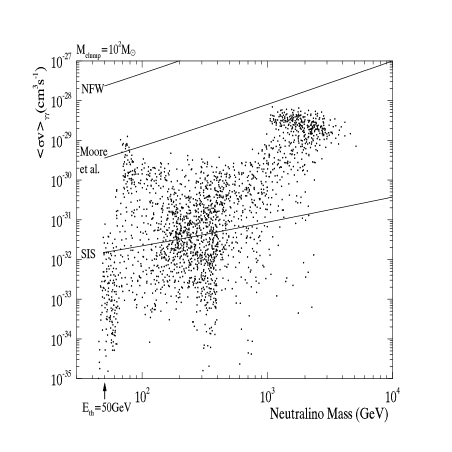
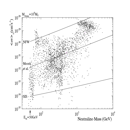
The way the constraints imposed on the SUSY parameter space depend on the mass of the clump is depicted in FIG.2, assuming a Moore et al. density profile, and for the same observation parameters as in FIG.1. The results are plotted for four different clump masses: , , and . As evident, the higher mass clumps have better chances of detectability, since the higher the mass of the clump, the larger the part of the SUSY parameter space that lies above the minimum detectable cross section, , versus curve; equivalently, the higher the mass, the stronger the constraints on the SUSY parameter space that the non-detectability of an otherwise detected clump (via e.g. its synchrotron emission bot02 ) imposes, given that if the clump is not detected by ACTs, all the models above the - curve will be excluded.
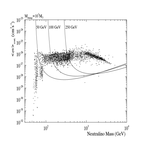
The minimum neutralino mass that can be explored also depends on the observation features, and more importantly, on the energy threshold. To show the role of the energy threshold, , in the detectability of the clumps for the SUSY parameter space, in FIG.3 we plot the same kind of curves as in previous figures, using a Moore et al. clump and for three different energy thresholds: 50, 100 and 250 GeV, for 100 hrs of observation and for and in agreement with Table 3. Using a higher energy threshold means both a larger and a better angular resolution, as well as lower contributions from the backgrounds, which makes it clear that ACTs are well-suited to explore the higher range of the neutralino parameter space. On the other hand, the lower the energy threshold the larger the part of the parameter space that ACTs can explore, but even in the best case of the smallest energy threshold, the low mass parameter space which corresponds to a broad range of will remain unexplored regardless of the mass of the clump. This demonstrates the need for complementary observations at lower energies, such as observations with GLAST glast , accelerator searches, and direct searches.
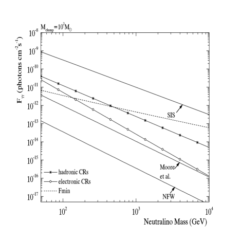
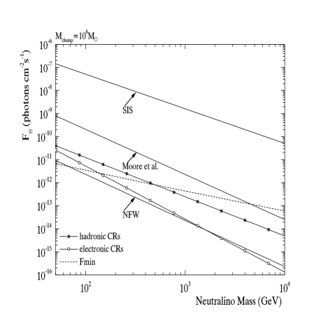
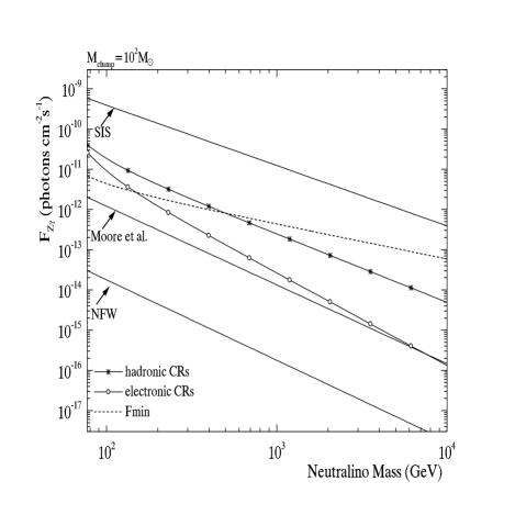
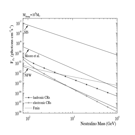
Our second set of results concerns the flux coming from a clump as a function of neutralino mass. Following the trend given by the DarkSUSY models, we choose a typical cross section for the annihilation into the continuum cm3 s-1. Note that the SUSY parameter space is not extremely wide in the continuum case, at least for neutralino masses above 80 GeV, and thus the choice of a typical cross section is reasonable. The flux as a function of for , and for clump masses and is shown in FIG.4. As above, we show the results for the three different density profiles we used. The energy threshold was set to GeV. On the same plot and for the same energy threshold, the electronic and hadronic backgrounds, as well as the 5- minimum detectable flux, (defined in Eq.(40)), are plotted using cm2 and s hrs. In these plots a clump of a specific mass and density profile will be detectable for those neutralino masses for which its flux is greater or equal to the minimum detectable flux . We will call this range of neutralino masses the detectability range.
From FIG.4, we see that a NFW clump will not be detectable (regardless of ), an SIS clump of the same mass has an detectability range GeV, whereas if the clump density distribution is better described by a Moore et al. profile, the detectability range will be GeV TeV, approximately. In the case of a clump, the SIS profile has an detectability range GeV. Similarly for the Moore et al. clump GeV, whereas the same clump if modeled with an NFW profile will have an detectability range GeV TeV. Focusing on the intermediate case, the Moore et al. profile, we see that in terms of constraints on , the detectability of low mass clumps provide both a lower and an upper limit (i.e., detectability range of the form ), whereas the higher-mass clump detectability provides only a weaker lower limit (i.e., detectability range of the form ). Note that the same conclusions if applied in the case of a clump known to exist but which turns out to be non-detectable by ACTs, imply complementary to the above limits for the neutralino parameter space. Namely, the non-detectability of the clump will imply that lies in the range : all values predicted by SUSY detectability range. Actually, as can be seen from all figures referring to the continuum signal, it will be the non-detectability that will impose the strongest constraints on the SUSY parameter space. Furthermore, although the larger the clump mass the easier to detect, having a range of clump masses is needed in order to determine the neutralino parameters. As we discuss below, the constraints can become stronger when information on the line emission is combined with the better detectable continuum -rays.
Lastly, given the SUSY parameter space and the dependence of the flux, we find the minimum and maximum flux above GeV that a clump of a specific mass and density profile can emit. We do that by finding from the SUSY parameter space what and combinations yield the minimum and maximum ratio, respectively. In this way, we bracket the flux of a clump and we know that, even for density profiles other than the three ones used here, as long as they are somewhere between the NFW and the SIS, their flux will be somewhere in the interval . The results of this calculation are shown in Table 4. For the minimum possible clump flux, , we chose TeV and cm3 s-1. This combination yields a representative lower flux value, at least for the horizontal feature of SUSY models in the large range (even lower fluxes are obtained for the low mass and low cross section part of the SUSY parameter space, but this range is not likely to be accessible by ACTs, anyway). For the maximum possible clump flux, , we used GeV and cm3 s-1, which is a combination that quite reliably gives the maximum possible flux. For comparison, in Table 5 we give the minimum required flux, , so that a 5- detection be obtained for certain and combinations, as was calculated using Eq. (40) and assuming the hadronic and electronic backgrounds as the dominant ones.
| SIS | |||||
|---|---|---|---|---|---|
| Moore | |||||
| NFW |
| t | |||
|---|---|---|---|
| 50 | |||
| 100 | |||
| 250 | |||
| 50 | |||
| 50 | |||
| 50 |
From the two tables we see that the least likely case of clumps, namely clumps as dense as the SIS, can be easily detectable in less than 100 hrs. In the case of the Moore et al. profile, the higher mass clumps () will be easily detectable since both and exceed the minimum required flux, , to achieve a 5- detection level. The lower mass clumps have an easily detectable , but not necessarily a detectable . A Moore et al. clump would have a detectable for either a large integration times ( s 1 month ), or for larger collective areas (e.g., at 50 GeV), which is not among the abilities of both existing and upcoming ACTs. Finally, NFW clumps with are detectable and this is particularly important given the EGRET constraints placed on the most concentrated clumps, such as SIS and Moore et al. ones. In contrast, even a whole year of observation (s) would not be enough to detect smaller mass NFW clumps with fluxes that are closer to the corresponding .
V.3 Monochromatic -rays
The minimum detectable cross section for annihilation into monochromatic -rays with energy equal to , as a function of is shown for and in FIG.5. The constraining curves stop at , which in this case is 50 GeV (below this the cross section is non-zero, but the number of photons with energy above 50 GeV coming from neutralinos with mass less than 50 GeV is, of course, 0). A first, clear difference, in comparison with the continuum -rays, is the fact that the SUSY parameter space is significantly wider with respect to the cross section. Therefore, imposing constraints on the SUSY parameter space using the detectability (or non-detectability) of the clumps through their line emission will be harder than through their continuum emission. Nevertheless, if lines are detected in addition to the continuum, the degeneracy in the SUSY parameter space will be lifted since a narrower range of models would fit both detections.
This is depicted more quantitatively in FIG.6 where we present the flux of monochromatic -rays as a function of , as well as the minimum detectable flux and the two major background contributions. Note that in this case both the minimum detectable flux and the background fluxes depend on , given that the energy of the monochromatic -rays is equal to . As we did in the case of the continuum, to find the flux coming from a given clump we assume a typical cross section, in order to express the flux only as a function of . Based on the SUSY parameter space presented in FIG.5, we choose the large cross section region and use cm3s-1. This value yields a flux close to the maximum possible flux such that a comparison can be attempted with the continuum case, which is generally stronger. We see, however, from FIG.6 that even in this case, the line will not be observable with upcoming ACTs. More specifically, for the chances of observing such a light clump in the monochromatic -ray lines are bad, regardless of neutralino mass. With respect to the density profile, neither the Moore et al. nor the NFW will be detectable. In the case of a density profile between the Moore et al. and the SIS, observability could be achieved imposing at the same time an upper limit on . In the case of , a Moore et al. clump will be detectable as long as 4.5 TeV, whereas the same clump, if described by an NFW profile, would be detectable only if 68 GeV.
The case is similar for the line. Results for the SUSY parameter space are presented in FIG.7, for and . In these figures we require that . Using the fact that , this implies that the neutralino mass
| (41) |
which translates to GeV for GeV. The two lines are expected to coincide at relatively large , and thus, the conclusions for both are similar with the difference that due to the above constraint the line explores the parameter space starting from higher neutralino masses compared to the line. In addition, the SUSY models corresponding to above 500 GeV are less dispersed in the case of the line than in the case of the . Again, this will help lift degeneracies of neutralino models, if any clumps are detected.
The flux as a function of neutralino mass assuming a maximum cm3 s-1, is shown in FIG.8. In general the conclusions are the same as in the line. The light clumps are not very promising with respect to their detectability. A Moore et al. clump will be detectable as long as 6 TeV. Note, however, that this is true under the assumption of the maximum , and thus of the maximum possible flux.
VI Discussion and Conclusions
The results presented above were based on specific choices for the detector and the observation parameters. It is worth noting that these results can be easily scaled with some of these parameters. For instance, the effective area and observation time have a simple scaling. The minimum detectable for a specific scales as . An order of magnitude lower could be explored using two orders of magnitude higher , for example, cm2 and s ( 40 days). This would be very helpful in the case of the hard to detect lines (see FIG.5 and FIG.7). If some clumps are detected in the continuum, a reasonable strategy would be to subsequently search for the weaker line signal over a longer . Similarly, the minimum detectable flux plotted in FIGs.4, 6, and 8, depends on the combination . With respect to the angular resolution , the minimum detectable has a dependance of the form , approximately, while the minimum detectable fluxes are . Note that although the nearest clumps are resolved, we used the angular resolution of the instrument and not the angular size of the clumps as the relevant angle for the collection of background noise, assuming that we observe the central pixel of the source – where most of the source counts originate from – treating thus, the source with respect to the backgrounds as being effectively unresolved. If, instead, one uses the angular size of the object as the relevant angle for the collection of noise, both the detectable cross sections and the minimum detectable fluxes are about two and one orders of magnitude higher for a and a clump, respectively.
An essential parameter in our calculations is the distance of the source from the Earth, which we assumed to be the estimated distance to the nearest clump. However, our results can be easily extended to larger distances or, equivalently, to lower numbers of clumps given the dependence of the flux, which is actually the most significant dependence of our results on the distance three . For example, one order of magnitude larger distance makes the minimum that can be explored two orders of magnitude higher; the same is true for the minimum detectable fluxes. This is very useful given the recent bounds on SIS and Moore et al. clumps from EGRET data abo02 . More specifically, only NFW clumps can populate the whole halo as seen in CDM simulations without overwhelming EGRET limits. For the other density profiles, consistency with EGRET data could imply, e.g., a smaller than currently believed clump abundance, which would translate, in our case, to larger distances of the clumps. Using the above scaling of our results with distance, it is easy to conclude with respect to the clump detectability in any other case that would change the distance estimate. Similar is the case for the density profile assumed for the clumps; the detectability of a density profile, e.g., with central concentration in between that of the Moore at al. and the NFW profiles, can be predicted, at least qualitatively, using our results.
The choice of the energy threshold will be a crucial factor determining what will be the minimum values accessible to ACTs. An energy threshold low enough, along with the ability of ACTs to identify primaries leading thus to backgrounds smaller by an order of magnitude, are highly desirable for future ACTs, if they are to be used to explore the SUSY parameter space and detect even the less concentrated clumps such as the NFW case.
In addition, we would like to re-emphasize the strategy of combining observations in the continuum and the annihilation lines for different clump masses in order to constrain more effectively the SUSY parameter space. For example, from FIGs.4 and 6 we saw that a low mass clump has an detectability range of the form . Combining this with line observations, one could narrow the range of neutralino masses. More precisely, one should study the allowed models in SUSY parameter space that fit the detected continuum flux and check which ones give a detectable line signal.
The detectability of the lines can yield detectability ranges of the form for various combinations of clumps masses and density profiles, assuming a typical or an optimum for the neutralino annihilation. Assuming for the lines the maximum , a Moore et al. clump will be detectable both in the continuum and in the lines, if is somewhere between 65 GeV and 4.5 TeV, where 65 GeV comes from the continuum limit and 4.5 TeV comes from the lines. Although not a very narrow interval in , excluding the very low mass end of the allowed neutralino mass range in combination with an upper -limit for detectability, can be very useful. It would narrow down the range in significantly. Another example is that of a NFW clump which is detectable in either the continuum ( detectability range: 77 GeV 5 TeV) or the line (detectability range: 68 GeV), but not both. This fact can, in principle, be used to extract information about the mass of the clump.
Our study of the detectability of clumps by ACTs is closely tied to the lack of knowledge with respect to the SUSY parameters. Thus our results can be used in two ways, depending mainly on what will be determined first, the neutralino parameters or the distribution and profiles of CDM clumps. If clumps are discovered first (for example, through synchrotron emission or from GLAST -ray observations), -ray studies by ACTs can help narrow the neutralino parameter space. In most cases, the strongest constraints on the SUSY parameter space arise from the non-detectability in -rays of a clump seen, e.g., in the microwaves bot02 rather than its detectability as, for example, in the case of a Moore et al. clump. Such a clump will be detectable in both the continuum and the lines if is between 65 and 4.5 TeV. This large range of neutralino masses can be ruled out if the clump is not detected by VERITAS. This can become quite useful in the future. For the time being, what is even more important is that such a clump, if existent, will be easily detectable almost for any possible neutralino mass.
Summarizing, we conclude that the chances of detectability of dark matter clumps in the galactic halo, due to continuum -rays produced by neutralino annihilation via upcoming ACTs are very good, especially in the case of relatively massive and highly centrally concentrated clumps. The signatures expected in the form of the and the lines are less easily detectable, but can be quite useful in lifting degeneracies among neutralino SUSY parameters. If we figure out the neutralino parameters first, ACT searches will be strong tests of the CDM model predictions with respect both the substructure in galactic halos and the density profiles of the substructure clumps. ACT searches will be able to explore large ranges of neutralino masses above 50 GeV (or more, depending on the energy threshold). These studies will complement the searches for lower mass neutralinos, accessible through high energy accelerators, direct and other indirect detection methods, and satellite -ray telescopes such as GLAST.
Acknowledgements
We thank Paolo Gondolo for help with DarkSUSY and Roberto Aloisio, Pasquale Blasi, and Craig Tyler, for many interesting discussions. This work was supported in part by the NSF through grant AST-0071235 and DOE grant DE-FG0291-ER40606 at the University of Chicago and at the Center for Cosmological Physics by grant NSF PHY-0114422.
References
- (1) G. Jungman, M. Kamionkowski, K. Griest, Phys. Rep. 267, 195 (1996).
- (2) J. Ellis, T. Falk, G. Ganis, K. A. Olive, Phys. Rev. D62, 075010 (2000).
- (3) V. Berezinsky, A.V. Gurevich, K.P. Zybin, Phys. Lett. B294, 221 (1992).
- (4) V. Berezinsky, A. Bottino, G. Mignola, Phys. Lett. B325, 136 (1994).
- (5) P. Gondolo, J. Silk, Phys. Rev. Lett. 83, 1719 (1999).
- (6) P. Gondolo, hep-ph/0002226.
- (7) G. Bertone, G. Sigl, J. Silk, MNRAS 326, 799 (2001).
- (8) L. Bergström, J. Edsjö, P. Gondolo, P. Ullio, Phys. Rev. D59, 043506 (1999).
- (9) C. Calcáneo–Roldán, B. Moore, astro-ph/0010056.
- (10) R. Aloisio, P. Blasi, A.V. Olinto, astro-ph/0206036.
- (11) P. Blasi, A.V. Olinto, C. Tyler, astro-ph/0202049.
- (12) C. Tyler, astro-ph/0203242
- (13) D. Merritt, M. Milosavljevic, in DARK 2002: 4th International Heidelberg Conference on Dark Matter in Astro and Particle Physics, 4-9 Feb 2002, Cape Town, South Africa, H.V. Klapdor-Kleingrothaus, R. Viollier (eds.) and astro-ph/0205140.
- (14) S. Ghigna, B. Moore, F. Governato, G. Lake, T. Quinn, J. Stadel, MNRAS 300, 146 (1998).
- (15) B. Moore, S. Ghigna, F. Governato, G. Lake, T. Quinn, J. Stadel, P. Tozzi, Ap.J. Lett. 524, L19 (1999).
- (16) A. Klypin, A.V. Kravtsov, O. Valenzuela, F. Prada, Ap.J., 522, 82 (1999).
- (17) A. Tasitsiomi, astro-ph/0205464.
- (18) V.V. Vassiliev et al., 26th ICRC, (Salt Lake City), 5, 299 (1999); http://veritas.sao.arizona.edu
- (19) W. Hofmann, GeV-TeV Gamma Ray Astrophysics Workshop, Snowbird, UT. (1999); AIP Proc. Conf. 515, 492 (1999).
- (20) M. Martinez, 26th ICRC, (Salt Lake City), 5, 219 (1999).
- (21) M. Mori et al., GeV-TeV Gamma Ray Astrophysics Workshop, Snowbird, UT. (1999); AIP Proc. Conf. 515, 485 (1999).
- (22) A.S. Font, J.F. Navarro, J. Stadel, T. Quinn, Ap.J. 563, L1 (2001).
- (23) I.R. Walker, J.C. Mihos, L. Hernquist, Ap.J. 460, 121 (1996).
- (24) H. Velazquez, S.D.M. White, MNRAS 304, 254 (1999).
- (25) P. Blasi, R.K. Sheth, Phys. Lett. B486, 233 (2000).
- (26) G. Lake, Nature 346, 39 (1990).
- (27) L. Bergström, J. Edsjö, P. Gondolo, P. Ullio, Phys. Rev. D59, 043506 (1999).
- (28) J.F. Navarro, C.S. Frenk, S.D.M. White, Ap.J. 462, 563 (1996).
- (29) A. Klypin, A.V. Kravtsov, J. Bullock, J.R. Primack, Ap.J. 554, 903 (2001).
- (30) J.E. Taylor, J.F. Navarro, Ap.J. 563, 483 (2001).
- (31) J.F. Navarro, astro-ph/0110680.
- (32) J. Binney, S. Tremaine, Galactic Dynamics, p. 452 (Princeton:Princeton University Press).
- (33) Similar is the conclusion with respect to the mass, , that appears in Eq.(8). Namely, for the distances from the galactic center that are relevant here, both profiles yield similar results.
- (34) More generally, for an behavior of the density profile at the center, the contribution of the core to the flux scales as , which implies a sensitive dependence on for , assuming of course that . Note however that the behavior of the density profile at intermediate distances () might also be important in some cases in determining the overall dependence of the flux on .
- (35) E.A. Baltz, C. Briot, P. Salati, R. Taillet, J. Silk, Phys. Rev. D61, 023514 (1999).
- (36) L. Bergström, J. Edsjö, C. Gunnarsson, Phys. Rev. D63, 083515 (2001).
- (37) J. Edsjö, P. Gondolo, Phys. Rev. D56, 01879 (1997).
- (38) DarkSUSY, http://www.physto.se/edsjo/dark susy, P.Gondolo, J. Edsjö, L.Bergström, P.Ullio, E.A. Baltz, in preparation.
- (39) L. Bergström, P. Gondolo, Astrop.Phys. 5, 263 (1996).
- (40) L. Bergström, P. Ullio, Nucl. Phys. B504, 27 (1997).
- (41) P. Ullio, L. Bergström, Phys. Rev. D57, 1962 (1998).
- (42) M. Drees, M.M. Nojiri, D.P. Roy, Y.Yamada, Phys. Rev. D56, 276 (1997).
- (43) S. Heinemeyer, W. Hollik, G. Weiglein, Phys. Lett. B455, 179 (1999); http://www-itp.physik.uni- karlsruhe.de/feynhiggs/
- (44) P. Gondolo, G. Gelmini, Nucl. Phys. B360, 145 (1991).
- (45) J.A. Peacock, Cosmological Physics, section 3.2 (Cambridge: Cambridge University Press).
- (46) A.G. Reiss et al., A.J. 116, 1009 (1998).
- (47) S. Perlmutter et al., Ap.J. 517, 565 (1999).
- (48) C.T. Hill , Nucl. Phys. B224, 469 (1983).
- (49) C.T. Hill, D.N. Schramm, T.P. Walker, Phys. Rev. D36, 1007 (1987).
- (50) For simplicity, from that point on we will use the term cross section to denote the thermally averaged product of the cross section times the relative velocity.
- (51) In fact, the low (good) VERITAS resolution – which renders the nearest clumps resolved – has been a crucial factor in determining our strategy, namely, the use of individual clumps rather than of all-sky maps that might be more appropriate in the case of numerous, unresolved clumps, as most clumps would appear when observed via instruments of higher (worse) angular resolution, e.g., GLAST.
- (52) L. Bergström, P. Ullio, J.H. Buckley, Astrop.Phys. 9, 137 (1998 ).
- (53) M.S. Longair, High Energy Astrophysics (Cambridge: Cambridge University Press).
- (54) P. Sreekumar et al., Ap.J. 494, 523 (1998).
- (55) S.D. Hunter et al., Ap.J. 481, 205 (1997).
- (56) L. Bergström, J. Edsjö, C. Gunnarsson, Phys. Rev. D63, 083515 (2001).
- (57) D.A. Kniffen, D.L. Bertsch, N. Gehrels, GeV-TeV Gamma Ray Astrophysics Workshop, Snowbird, UT. AIP Proc. Conf. 515, 492 (1999).
- (58) Other weaker dependencies exist as, for example, via Eqs.(7) and (21).