THESIS
The Pursuit of Non-Gaussian Fluctuations
in the Cosmic Microwave Background

A dissertation submitted to
Tohoku University
in partial fulfillment of requirements for the degree of
Doctor of Philosophy
in
Science

Eiichiro Komatsu
Astronomical Institute, Tohoku University

Abstract

We present theoretical and observational studies of non-Gaussian fluctuations in the cosmic microwave background (CMB) radiation anisotropy. We use the angular bispectrum and trispectrum, the harmonic transform of the angular three- and four-point correlation functions. If the primordial fluctuations are non-Gaussian, then this non-Gaussianity will be apparent in the CMB sky.

Non-linearity in inflation produces the primordial non-Gaussianity. We predict the primary angular bispectrum from inflation down to arcminutes scales, and forecast how well we can measure the primordial non-Gaussian signal. In addition to that, secondary anisotropy sources in the low-redshift universe also produce non-Gaussianity, so do foreground emissions from extragalactic or interstellar microwave sources. We study how well we can measure these non-Gaussian signals, including the primordial signal, separately. We find that when we can compute the predicted form of the bispectrum, it becomes a “matched filter” for finding non-Gaussianity in the data, being very powerful tool of measuring weak non-Gaussian signals and of discriminating between different non-Gaussian components. We find that slow-roll inflation produces too small bispectrum to be detected by any experiments; thus, any detection strongly constrains this class of models. We also find that the secondary bispectrum from coupling between the Sunyaev–Zel’dovich effect and the weak lensing effect, and the foreground bispectrum from extragalactic point sources, give detectable non-Gaussian signals on small angular scales.

We test Gaussianity of the COBE DMR sky maps, by measuring all the modes of the angular bispectrum down to the DMR beam size. We compare the data with the simulated Gaussian realizations, finding no significant signal of the bispectrum on the mode-by-mode basis. We also find that the previously reported detection of the bispectrum is consistent with a statistical fluctuation. By fitting the theoretical prediction to the data for the primary bispectrum, we put a constraint on non-linearity in inflation. Simultaneously fitting the foreground bispectra, which are estimated from interstellar dust and synchrotron template maps, shows that neither dust nor synchrotron emissions contribute significantly to the bispectrum at high Galactic latitude. We thus conclude that the angular bispectrum finds no significant non-Gaussian signals in the DMR data.

We present the first measurement of the angular trispectrum on the DMR sky maps, further testing Gaussianity of the DMR data. By applying the same method as used for the bispectrum to the DMR data, we find no significant non-Gaussian signals in the trispectrum. Therefore, the angular bispectrum and trispectrum show that the DMR sky map is comfortably consistent with Gaussianity.

The methods that we have developed in this thesis can readily be applied to the MAP data, and will enable us to pursue non-Gaussian CMB fluctuations with the unprecedented sensitivity. We show that high-sensitivity measurement of the CMB bispectrum and trispectrum will probe the physics of the early universe as well as the astrophysics in the low-redshift universe, independently of the CMB power spectrum.

Contents

1. 1 Introduction
   1. 1.1 Why Pursue Non-Gaussianity in CMB?
   2. 1.2 Inhomogeneity in Microwave Sky
      1. 1.2.1 COBE DMR sky maps
      2. 1.2.2 Post-COBE era
   3. 1.3 Non-Gaussian Fluctuations in Inflation
      1. 1.3.1 Adiabatic production of non-Gaussian fluctuations
      2. 1.3.2 Isocurvature fluctuations
2. 2 Perturbation Theory in Inflation
   1. 2.1 Inflation—Overview
   2. 2.2 Quantum Fluctuations
      1. 2.2.1 Quantization in de Sitter spacetime
      2. 2.2.2 Scale-invariant fluctuations on super-horizon scales
      3. 2.2.3 Tilted “red” spectrum
      4. 2.2.4 Emergence of classical fluctuations
   3. 2.3 Linear Perturbation Theory in Inflation
      1. 2.3.1 Fluid representation of scalar field
      2. 2.3.2 Gauge-invariant perturbations
      3. 2.3.3 Generation of spatial curvature perturbations
      4. 2.3.4 Generation of primary CMB anisotropy
   4. 2.4 Non-linear Perturbations in Inflation
      1. 2.4.1 Gradient expansion of Einstein equations
      2. 2.4.2 Generation of non-linear curvature perturbations
      3. 2.4.3 Generation of weakly non-Gaussian adiabatic fluctuations
3. 3 Angular $n$-point Harmonic Spectrum on the Sky
   1. 3.1 Statistical Isotropy of the Universe
   2. 3.2 Angular Power Spectrum
      1. 3.2.1 Estimator
      2. 3.2.2 Covariance matrix
   3. 3.3 Angular Bispectrum
      1. 3.3.1 Estimator
      2. 3.3.2 Covariance matrix
   4. 3.4 Angular Trispectrum
      1. 3.4.1 Estimator
      2. 3.4.2 Covariance matrix
   5. 3.5 Power Spectrum and Bispectrum on the Incomplete Sky
4. 4 Theoretical Predictions for the CMB Bispectrum
   1. 4.1 Reduced Bispectrum
   2. 4.2 Primary Bispectrum and Skewness
      1. 4.2.1 Model of the primordial non-Gaussianity
      2. 4.2.2 Numerical results of the primary bispectrum
      3. 4.2.3 Primary skewness
   3. 4.3 Secondary Sources of the CMB Bispectrum
      1. 4.3.1 Coupling between the weak lensing and the Sunyaev–Zel’dovich effects
      2. 4.3.2 Extragalactic radio and infrared sources
   4. 4.4 Measuring Bispectra
      1. 4.4.1 Fisher matrix
      2. 4.4.2 Measuring primary bispectrum
      3. 4.4.3 Measuring secondary bispectra
      4. 4.4.4 Measuring primary skewness
   5. 4.5 Discussion and Conclusions
5. 5 Measurement of Bispectrum on the COBE DMR sky maps
   1. 5.1 Angular Bispectrum
   2. 5.2 Measurement of Bispectrum on the DMR Sky Maps
      1. 5.2.1 The data
      2. 5.2.2 Monte–Carlo Simulations
      3. 5.2.3 Normalized bispectrum
      4. 5.2.4 Testing Gaussianity of the DMR map
   3. 5.3 Model Fitting
      1. 5.3.1 Primary bispectrum
      2. 5.3.2 Foreground bispectra from interstellar emissions
      3. 5.3.3 Constraints on non-linearity in inflation
      4. 5.3.4 Null test of the normalized bispectrum
   4. 5.4 Discussion and Conclusions
6. 6 In Pursuit of Angular Trispectrum
   1. 6.1 Angular Trispectrum
   2. 6.2 Normalized Trispectrum
   3. 6.3 Testing Gaussianity of the DMR Map
      1. 6.3.1 Classification of trispectrum configurations
      2. 6.3.2 Gaussianity test

List of Figures

1. 1.1 COBE DMR Sky Map
2. 1.2 COBE DMR Angular Power Spectrum
3. 1.3 COBE DMR, QMASK, and BOOMERanG Angular Power Spectra
4. 1.4 Sub-degree CMB Maps: BOOMERanG and QMASK
5. 1.5 Three Steps for Non-Gaussian CMB Anisotropy
6. 1.6 Adiabatic Non-Gaussianity: One-point p.d.f
7. 1.7 Isocurvature Non-Gaussianity: One-point p.d.f
8. 2.1 Classical Evolution of Scalar Field
9. 2.2 Physical Length Scales in Cosmic Evolution
10. 2.3 Color of Spectrum
11. 2.4 The Static Sachs–Wolfe Effect
12. 2.5 Hypersurface Transformation
13. 3.1 Ensemble Average of Angular Correlation Function
14. 3.2 Statistical Isotropy of Angular Correlation Function
15. 3.3 Angular Bispectrum Configuration
16. 3.4 Variance of Angular Bispectrum
17. 3.5 Angular Trispectrum Configuration
18. 3.6 Variance of Angular Trispectrum I
19. 3.7 Variance of Angular Trispectrum II
20. 4.1 Components of Primary CMB Bispectrum
21. 4.2 Primary CMB Bispectrum
22. 4.3 Primary Skewness
23. 4.4 SZ–lensing Coupling
24. 4.5 Equilateral Reduced Bispectra
25. 4.6 Signal-to-noise Ratio
26. 4.7 Bispectrum vs Skewness
27. 5.1 Variance of Normalized Bispectrum and Bare Bispectrum
28. 5.2 Distribution of Bispectrum
29. 5.3 Distribution of Normalized Bispectrum
30. 5.4 KS Test for Gaussianity with Bispectrum
31. 5.5 Constraint on Non-linearity in Inflation
32. 5.6 Constraint on Dust Bispectrum
33. 5.7 Constraint on Synchrotron Bispectrum
34. 5.8 Null Test of Normalized Bispectrum
35. 6.1 Variance of Normalized Trispectrum and Bare Trispectrum
36. 6.2 KS Test for Gaussianity with Trispectrum I
37. 6.3 KS Test for Gaussianity with Trispectrum II

List of Tables

1. 4.1 Fisher Matrix
2. 4.2 Inverted Fisher Matrix
3. 4.3 Signal-to-noise Ratio
4. 4.4 Signal Degradation and Correlation Matrix
5. 4.5 Detection Limit for the Non-linear Coupling Parameter
6. 5.1 Monopole and Dipole Subtraction
7. 6.1 Gaussianity Test with Normalized Trispectrum

Chapter 1 Introduction

1.1 Why Pursue Non-Gaussianity in CMB?

Modern understanding to emergence of inhomogeneity in the universe through the cosmic history is outstanding; the inhomogeneity is quantum in origin. Then, it becomes classical through its evolution, producing fluctuations in the cosmic microwave background (CMB) radiation, and creating complex structures, such as galaxies, seen in the present universe.

A theory of early universe, the cosmic inflation (Guth81; Sato81; AS82; Lin82), has predicted the emergence of the quantum fluctuations in early universe. Inflation not only resolves several serious issues in the old Big-Bang cosmology, but also gives a mechanism to produce inhomogeneity in the universe, and makes specific testable predictions for the global structure and the inhomogeneity in the universe (GP82; Haw82; Sta82; BST83). The predictions may concisely be summarized as follows:

• The observable universe is spatially flat.

• The observable universe is homogeneous and isotropic on large angular scales, apart from tiny fluctuations.

• The primordial inhomogeneity has a specific spatial pattern, so-called the scale-invariant fluctuation.

• Statistics of the primordial inhomogeneity obey Gaussian statistics.

All these predictions but (d) have passed challenging observations. Among those observations, the most firm evidence supporting the predictions has come from measurement of the angular distribution of CMB. Being the oldest observable object in the universe, CMB is the best clue to early universe.

Observed isotropy of CMB with 0.001% accuracy supports the prediction (b) (Mat90; Smo92). The measured angular distribution of the CMB anisotropy, 0.001% inhomogeneity, supports the primordial fluctuation distribution being consistent with the prediction (c) in the flat universe, the prediction (a) (Ben96; TOCO99; Boom00; Maxima00).

Using various statistical techniques, many authors have attempted to test the prediction (d), the Gaussianity of the primordial inhomogeneity, using the CMB anisotropy on large angular scales ($\sim 7^{\circ}$) (Kog96b; FMG98; PVF98; BT99; BZG00; MHL00; Mag00; SM00; Bar00), on intermediate scales ($\sim 1^{\circ}$) (Park01), and on small scales ($\sim 10^{\prime}$) (Wu01).

In contrast to the predictions (a)–(c) for which the observations suggest no controversy, previous work on searching for non-Gaussian CMB anisotropies has come to different conclusions from one another: some do claim detection (FMG98; PVF98; Mag00), and the others do not (Kog96b; SM00; Bar00; Park01; Wu01). Furthermore, BT99 and BZG00 claim the non-Gaussian signal of FMG98 to be non-cosmological in origin. MHL00 revise the conclusion of PVF98 by addressing ambiguity in their method, from which the conclusion crucially depends upon an orientation of the data on the sky, and show no evidence for the non-Gaussianity. The existence of non-Gaussianity in CMB is controversial.

Since non-Gaussianity has infinite degrees of freedom, testing a Gaussian hypothesis is difficult; one statistical method showing CMB consistent with Gaussian does not mean CMB being really Gaussian. In this sense, different statistical methods can come to different conclusions. In addition to the difficulty, cosmological non-Gaussianity is hard to measure. Instrumental and environmental effects in observations easily produce spurious non-Gaussian signals. Astronomical microwave sources such as interstellar dust emissions also produce strong non-Gaussian fluctuations on the sky. Hence, we must be as careful as possible when searching for cosmological non-Gaussianity.

Pursuit of cosmological non-Gaussianity in CMB is a challenging test of inflation, the origin of inhomogeneity in the universe. In this dissertation, we present theoretical and observational studies of the CMB non-Gaussianity. Our primary goal is to test inflation with non-Gaussian CMB fluctuations.

As a statistical tool of searching for non-Gaussianity, we use the angular three- and four-point correlation functions in harmonic space, the angular bispectrum and trispectrum, which are sensitive to weakly non-Gaussian fluctuations. An advantage of these angular $n$-point harmonic spectra over other statistics is that they are predictable from not only inflation, but also secondary sources in the low-redshift universe (the Sunyaev–Zel’dovich effect, weak gravitational lensing effect, and so on), extragalactic foreground emissions, global topology of the universe, and so on. When we fit those predictions to the measured spectra, the predictions become “matched filters” for detecting weak non-Gaussianity in the data, and much more powerful than just a null test of Gaussianity.

This dissertation is organized as follows. The rest of this chapter will overview what the CMB sky looks like, and the previous study of CMB non-Gaussianity, followed by a heuristic description of non-Gaussian fluctuation production in inflation.

In chapter 2, we go through primordial fluctuation generation mechanism in inflation, and investigate how non-linear curvature perturbations are generated and propagated through the CMB anisotropy. We present a possible quantum-to-classical transition mechanism of the quantum fluctuations on super horizon scales.

In chapter 3, we study statistical properties of the angular $n$-point harmonic spectrum for $n=2$ (power spectrum), 3 (bispectrum), and 4 (trispectrum). We present practical methods of measuring the angular bispectrum and trispectrum from observational data with many pixels.

In chapter 4, we make theoretical predictions for the CMB angular bispectrum, which include primary contribution from inflation, secondary contribution from the Sunyaev–Zel’dovich effect and the weak-lensing effect, and foreground contribution from extragalactic radio and infrared astronomical sources. We estimate signal-to-noise ratios of detecting each contribution with CMB experiments, further discussing how well we can measure each contribution separately.

In chapter 5, we measure the angular bispectrum on the COBE DMR four-year data, testing Gaussianity of the data. By fitting the theoretical prediction for the primary bispectrum to the data, we constrain non-linearity in inflation; also fitting foreground bispectra from interstellar microwave emissions takes into account the effect of non-Gaussian interstellar dust and synchrotron emissions at high Galactic latitude.

In chapter 6, we measure the angular trispectrum on the DMR data, further testing Gaussianity of the data.

1.2 Inhomogeneity in Microwave Sky

The cosmic microwave background radiation (CMB) is the isotropic microwave radiation filling the sky. The temperature is precisely measured to be 2.73 K (Mat90), and the peak intensity at $\nu=160~{}{\rm GHz}$ ($\lambda=1.9~{}{\rm mm}$) is $370~{}{\rm MJy~{}str^{-1}}$. What if subtracting this mean radiation from the sky, what are we left with, completely dark, literally nothing?

1.2.1 COBE DMR sky maps

The Differential Microwave Radiometer (DMR) mounted on the Cosmic Background Explorer (COBE), the satellite for full sky measurement of CMB launched by NASA in 1989, has revealed that what we are left with is the tiny inhomogeneity; the r.m.s. amplitude is about 30 $\mu$K (Smo92), 0.001% of the mean temperature.

Various statistical analyses on the DMR sky maps have shown the angular distribution of the CMB anisotropy remarkably consistent with the scale-invariant fluctuation, the prediction of inflation (Ben96; Gor96; Hin96; Wri96). The scale-invariant fluctuation implies that the r.m.s. amplitude of the CMB anisotropy is nearly independent of angular scales. DMR has measured 35 $\mu$K r.m.s. fluctuations on $7^{\circ}$ scale, 29 $\mu$K on $10^{\circ}$ scale (Ban97).

DMR comprises 3 dual-horn antennas working at 31.5, 53, and 90 GHz. The combination of 53 and 90 GHz maps gives the most sensitive sky map to CMB, while 31.5 GHz map is twice as noisier as the other channels. Figure 1.1 shows the combined DMR full sky map. The left shows the raw map in which the instrumental noise dominates appearance of the map; the right shows the smoothed map with the DMR beam in which the instrumental noise is filtered out, giving better appearance of CMB signals. The mean signal-to-noise ratio of hot and cold spots in the smoothed map is 2, while a few prominent spots have 3 to 4. Hence, we cannot say much about structures of the CMB anisotropy relying on the map basis; however, we can do say on the statistical basis.

Statistically, structures in the DMR map are inconsistent with pure instrumental noise; on the contrary, the structure has a distinct angular correlation pattern represented by the scale-invariant fluctuation. To quantify this, it is useful to calculate the angular power spectrum, $C_{l}$, the harmonic transform of the angular two-point correlation function, which measures how much fluctuation power exists on a given angular scale, $\theta\sim\pi/l$. Figure 1.2 plots the measured $C_{l}$ on the DMR map. What is actually plotted is $l(l+1)C_{l}/2\pi$, roughly mean squares of fluctuations at $l$. The scale-invariant fluctuation implies $C_{l}\propto\left[l(l+1)\right]^{-1}$ (P82), and hence $l(l+1)C_{l}$ remains constant (solid line), so do the data points in the figure; the data points fit the inflation’s prediction well. The dashed line shows a more accurate prediction, taking into account the effects of general relativistic photon-baryon fluid dynamics before the decoupling as well as of time evolution of gravitational potential field after the decoupling. The agreement with the data becomes better, further confirming that the DMR angular power spectrum is consistent with inflation.

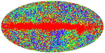
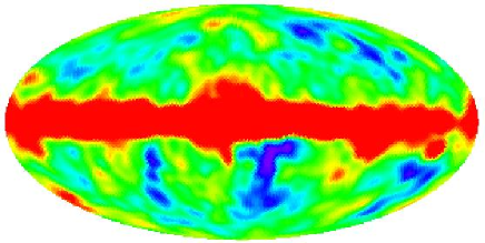
Figure 1.1: COBE DMR Sky Map

COBE DMR four-year $53+90$ GHz sky map in Galactic projection, using the HEALPix pixelization (GHW98) with $1.^{\circ}83$ pixel size, leaving 12,288 pixels. The left is the raw map, while the right map has been smoothed with a $7^{\circ}$ FWHM Gaussian.

Figure 1.2: COBE DMR Angular Power Spectrum

The CMB angular power spectrum, $C_{l}$, measured on the COBE DMR four-year map. The plotted quantity, $l(l+1)C_{l}/(2\pi)$, represents the r.m.s. amplitude of fluctuations at a given angular scale, $l$. The data points (filled circles) are uncorrelated with each other (TH97). The solid line shows the scale-invariant power spectrum, $l(l+1)C_{l}=\mbox{constant}$, while the dashed line shows a $\Lambda$CDM spectrum.

Gaussianity of the DMR data has been tested with various statistical methods (Kog96b; FMG98; PVF98; BT99; BZG00; MHL00; Mag00; SM00; Bar00). FMG98 and Mag00 claim positive detection of non-Gaussian signals using the angular bispectrum, and PVF98 claim detection using the wavelet analysis. The latter non-Gaussian signal has appeared to be less significant than they claim, as it disappears when the DMR map is rotated by $180^{\circ}$ (MHL00; Bar00). For the former two bispectrum analyses, BT99 and BZG00 claim that the FMG98’s signal is non-cosmological, but their claims do not account for the Mag00’s signal. In this thesis, we will argue that the reported non-Gaussian signals are not a matter of origin, but statistical fluctuations.

1.2.2 Post-COBE era

After the discovery of COBE, pursuit of the CMB anisotropy has been oriented toward measurement of the angular power spectrum, $C_{l}$, on smaller angular scales, i.e., larger $l$. Particularly, many efforts have been made to measure $C_{l}$ at $l\sim 200$ ($\theta\sim 1^{\circ}$), where inflation predicts a prominent peak in $l(l+1)C_{l}$ as a consequence of flatness of the universe, the prediction of inflation (KSS94).

By early 2000, there has been strong evidence for the peak (TOCO99); in the end of 2000, BOOMERanG and MAXIMA, balloon-borne CMB experiments, have detected the peak (Boom00; Maxima00), further supporting inflation. Figure 1.3 compares the data from three experiments, which probe different angular scales from one another, with a prediction from inflation. The agreement between the data and the prediction is outstanding.

Figure 1.3: COBE DMR, QMASK, and BOOMERanG Angular Power Spectra

The CMB angular power spectrum, measured by the three experiments probing different angular scales. The circles are the COBE DMR data (full sky coverage with a Galactic cut, $7^{\circ}$ angular resolution), the triangles are the QMASK data (648-square-degree sky coverage, $0.^{\circ}68$ angular resolution), and the squares are the BOOMERanG data (1,800-square-degree sky coverage, $0.^{\circ}17$ angular resolution). The dashed line shows a prediction of inflation, a $\Lambda$CDM spectrum with $\Omega_{\rm m}=0.3$, $\Omega_{\Lambda}=0.7$, $\Omega_{\rm b}=0.04$, $h=0.7$, and $n=0.95$.

Measurement of $C_{l}$ so far, however, has assumed CMB Gaussian. If CMB is not Gaussian, then the measured $C_{l}$ is biased. Moreover, when we fit the measured $C_{l}$ to a theoretical $C_{l}$, we need to know the covariance matrix of $C_{l}$. Since the covariance matrix of $C_{l}$ is the four-point harmonic spectrum, the trispectrum, we have to investigate non-Gaussian signals in the trispectrum to construct the covariance matrix accurately.

Even if non-Gaussianity is small, we have to take it into account in analyzing $C_{l}$; the next generation satellite experiments, MAP and Planck, will measure $C_{l}$ with 1% or better accuracy, and we will use the measured $C_{l}$ to determine many of cosmological parameters with 10% or better accuracy. Unless non-Gaussian effect is much smaller than the observational uncertainty (who knows?), we have to take the effect into account, to achieve the accurate measurement of the parameters.

The state-of-the-art balloon-borne experiments provide not only $C_{l}$, but also high resolution, high signal-to-noise ratio CMB maps. The left of figure 1.4 shows the BOOMERanG sky map, which covers roughly 3% of the sky, 1,800 square degrees, with $10^{\prime}$ ($0.^{\circ}17$) angular resolution. The high signal-to-noise ratios in the map show the observed structures in the map not instrumental noise, but CMB.

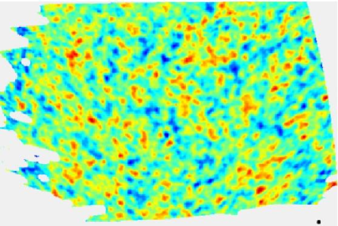
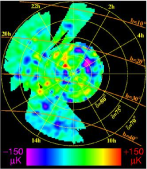
Figure 1.4: Sub-degree CMB Maps: BOOMERanG and QMASK

The left is the BOOMERanG sky map, which covers 3% of the sky, 1,800 square degrees, with $10^{\prime}$ ($0.^{\circ}17$) angular resolution (Boom00). The beam size is indicated by the filled circle at the bottom-right corner. The right is the QMASK sky map, which covers 648 square degrees of the sky with $0.^{\circ}68$ angular resolution (Xu01). Both maps have been scaled to match each other in size. The QMASK map is one-third of the BOOMERanG map.

Visually, the CMB anisotropy in the map looks very much Gaussian, implying non-Gaussianity is weak, if any. As yet the BOOMERanG team has not performed Gaussianity tests on the data; however, the MAXIMA team has done on their data. The MAXIMA map covers 124 square degrees of the sky with $10^{\prime}$ angular resolution, leaving 5,972 pixels. They have found that the one-point probability density distribution function and the Minkowski functionals measured on the map are consistent with Gaussianity.

The genus statistic has been applied to the QMASK map (Xu01), a high signal-to-noise ratio CMB map combining the balloon-borne QMAP (Qmap1; Qmap2; Qmap3) and the ground-based Saskatoon experiments (Sask97), showing the map consistent with Gaussian (Park01). The QMASK map is shown on the right of figure 1.4, where the size of the map has been scaled to match the BOOMERanG map. The QMASK map covers 648 square degrees of the sky, one-third of the BOOMERanG map, with $0.^{\circ}68$ angular resolution, leaving 6,495 pixels.

The number of independent pixels that has been used for Gaussianity tests on the DMR (3,881), MAXIMA (5,972), and QMASK (6,495) data is similar to each other; although their angular scales are quite different, they have similar power of testing Gaussianity. We will have a significant progress when the BOOMERanG data, in which the number of pixels is 57,103, test the Gaussianity.

The just-launched CMB satellite, the Microwave Anisotropy Probe (MAP), will increase our power of pursuing non-Gaussianity substantially. It will survey the full sky with the angular resolution better than $14^{\prime}$, and have $\lower 2.15277pt\hbox{$\;\buildrel>\over{\sim}\;$}10^{6}$ pixels. The statistical methods developed in this thesis can readily be applied to the MAP data, enabling us to test the Gaussianity with unprecedented sensitivity.

1.3 Non-Gaussian Fluctuations in Inflation

1.3.1 Adiabatic production of non-Gaussian fluctuations

While inflation predicts Gaussian CMB fluctuations to very good accuracy, strictly speaking, non-linearity in inflation produces weakly non-Gaussian fluctuations, which propagates through CMB. Although the exact treatment is complicated, we present a basic idea behind it concisely here (KS01b).

The curvature perturbations, $\Phi$, generate the CMB anisotropy, $\Delta T/T$. The linear perturbation theory gives a linear relation between $\Phi$ and $\Delta T/T$,

$$\frac{{\Delta T}}{T}\sim g_{\rm T}\Phi,$$ (1.1)

where $g_{\rm T}$ is the radiation transfer function. For temperature fluctuations on super-horizon scales at the decoupling epoch, the Sachs-Wolfe effect (SW67) dominates, and $g_{\rm T}=-1/3$ for adiabatic fluctuations. On sub-horizon scales, $g_{\rm T}$ oscillates (acoustic oscillation), and we need to solve the Boltzmann photon transport equations coupled with the Einstein equations for $g_{\rm T}$. It follows from the relation, $\Delta T\propto\Phi$, that $\Delta T$ is Gaussian, if $\Phi$ is Gaussian. As we will see, non-linearity in inflation makes $\Phi$ weakly non-Gaussian.

Even if $\Phi$ is Gaussian, $\Delta T/T$ can be non-Gaussian. According to the general relativistic cosmological perturbation theory, there is a non-linear relation between $\Delta T/T$ and $\Phi$:

$$\frac{{\Delta T}}{T}\sim g_{\rm T}\left(\Phi+f_{\Phi}\Phi^{2}\right).$$ (1.2)

Here, the second term with a coefficient of order unity, $f_{\Phi}\sim{\cal O}(1)$, is the higher-order correction arising from the second-order perturbation theory (PC96). It produces non-Gaussian fluctuations; thus, even if $\Phi$ is Gaussian, $\Delta T$ becomes weakly non-Gaussian.

Is $\Phi$ Gaussian? Non-linearity in inflation makes $\Phi$ weakly non-Gaussian. By expanding the fluctuation dynamics in inflation up to the second order, we obtain a non-linear relation between $\Phi$ and inflaton fluctuations, $\delta\phi$:

$$\Phi\sim m_{\rm pl}^{-1}g_{\Phi}\left(\delta\phi+m_{\rm pl}^{-1}f_{\delta\phi}\delta\phi^{2}\right).$$ (1.3)

SB90 show that this relation is a non-linear solution for curvature perturbations on super horizon scales; the solution gives $g_{\Phi}\sim{\cal O}(10)$ and $f_{\delta\phi}\sim{\cal O}(10^{-1})$ for a class of slowly-rolling single-field inflation models.

Quantum fluctuations produce Gaussian $\delta\phi$. If the dynamics of $\delta\phi$ is simple enough to keep itself Gaussian throughout the evolution, then we can stop our consideration here; however, it is not necessarily true. For example, non-trivial interaction terms in the equation of motion for inflaton fields (FRS93), or a non-linear coupling between long-wavelength classical fluctuations and short-wavelength quantum fluctuations in the context of stochastic inflation (Sta86; Gan94), can make $\delta\phi$ weakly non-Gaussian, resulting in a non-linear relation between $\delta\phi$ and a Gaussian field, $\eta$,

$$\delta\phi\sim g_{\delta\phi}\left(\eta+m_{\rm pl}^{-1}f_{\eta}\eta^{2}\right),$$ (1.4)

where $\eta$ represents initially produced quantum fluctuations, and $g_{\delta\phi}\sim 1$ and $f_{\eta}\sim{\cal O}(10^{-1})$. Figure 1.5 summarizes the above three steps in the opposite order.

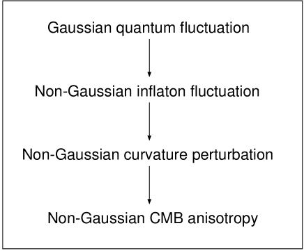
Figure 1.5: Three Steps for Non-Gaussian CMB Anisotropy

Adiabatic generation of non-Gaussian CMB anisotropies. First, inflation generates Gaussian quantum fluctuations, which become non-Gaussian inflaton fluctuations through a non-linear coupling between them (Eq.(1.4)). Then, the inflaton fluctuations become more non-Gaussian curvature perturbations through a non-linear relation between them (Eq.(1.3)). Finally, the curvature perturbations become more non-Gaussian CMB anisotropies through non-linear gravitational effects (Eq.(1.2)).

Collecting all the above contributions, we obtain a non-linear relationship between $\Delta T/T$ and $\Phi$,

$$\frac{{\Delta T}}{T}\sim g_{\rm T}\left[\Phi_{\rm L}+\left(f_{\Phi}+g_{\Phi}^{-1}f_{\delta\phi}+g_{\Phi}^{-1}g_{\delta\phi}^{-1}f_{\eta}\right)\Phi_{\rm L}^{2}\right],$$ (1.5)

where $\Phi_{\rm L}\equiv g_{\Phi}g_{\delta\phi}m_{\rm pl}^{-1}\eta\sim 10m_{\rm pl}^{-1}\eta$ is an auxiliary Gaussian curvature perturbation. It may be useful to define a non-linear coupling parameter, $f_{\rm NL}=f_{\Phi}+g_{\Phi}^{-1}f_{\delta\phi}+g_{\Phi}^{-1}g_{\delta\phi}^{-1}f_{\eta}$. The first term in $f_{\rm NL}$, the second order gravity effect $\sim{\cal O}(1)$, is dominant compared with the other two terms $\sim{\cal O}(10^{-2})$, non-linearity in slow-roll inflation. Note that $f_{\rm NL}$ corresponds to $-\Phi_{3}/2$ in Gan94 and $-\alpha_{\Phi}$ in VWHK00. Using $f_{\rm NL}$, we rewrite equation (1.5) as $\Delta T({\mathbf{x}})/T\sim g_{\rm T}\Phi({\mathbf{x}})$, where

$$\Phi({\mathbf{x}})=\Phi_{\rm L}({\mathbf{x}})+f_{\rm NL}\left[\Phi^{2}_{\rm L}({\mathbf{x}})-\left<\Phi^{2}_{\rm L}({\mathbf{x}})\right>\right],$$ (1.6)

the angular bracket denoting the statistical ensemble average.

To see intuitively what non-Gaussian fluctuations that we have considered here look like, in figure 1.6 we plot one-point probability density distribution function (p.d.f) of the CMB anisotropy. We compare Gaussian p.d.f with non-Gaussian p.d.f of adiabatic fluctuations produced in inflation. The dashed line is Gaussian distribution, i.e., no non-linear perturbations are included ($f_{\rm NL}=0$). The solid line includes non-linear coupling of order $f_{\rm NL}=1000$, while the dotted line of order $f_{\rm NL}=5000$. It follows from the figure that positive $f_{\rm NL}$ gives negatively skewed p.d.f; negative $f_{\rm NL}$ gives positively skewed p.d.f. The larger $\left|f_{\rm NL}\right|$ is, the more skewed p.d.f becomes.

Figure 1.6: Adiabatic Non-Gaussianity: One-point p.d.f

One-point probability density distribution function (p.d.f) of the CMB anisotropy, $\Delta T/T$, comparing a Gaussian p.d.f with non-Gaussian p.d.f’s of non-linear adiabatic fluctuations produced in inflation. The dashed line plots Gaussian distribution. The solid line plots non-Gaussian distribution for $f_{\rm NL}=1000$, the dotted line for $f_{\rm NL}=5000$. The larger $f_{\rm NL}$ is, the more negatively skewed p.d.f becomes. If $f_{\rm NL}<0$, then p.d.f becomes positively skewed.

We find that $f_{\rm NL}=1000$ gives virtually identical p.d.f to the Gaussian p.d.f. In chapter 4, we will show that even with the ideal CMB experiment, we can measure $\left|f_{\rm NL}\right|$ no smaller than 60, if we use the skewness of the one-point p.d.f. If we use the bispectrum, however, we can measure as small $\left|f_{\rm NL}\right|$ as 3. The bispectrum is thus much more sensitive to the adiabatic non-Gaussianity than the skewness of the one-point p.d.f is. In chapter 5, we will show that the angular bispectrum measured on the COBE DMR sky map constrains $\left|f_{\rm NL}\right|<1.6\times 10^{3}$. The next generation satellite experiments, MAP and Planck, will improve the constraint substantially.

Since the minimum $\left|f_{\rm NL}\right|$ detectable with CMB experiments is 3, the second order gravity effect, $f_{\rm NL}\sim{\cal O}(1)$, will not produce detectable non-Gaussianity in CMB, nor will slow-roll inflation, $f_{\rm NL}\sim{\cal O}(10^{-2})$.

Yet, inflation may not be so simple. Any significant deviation from slow-roll, or features in an inflaton potential (KBHP91), could produce a bigger $\left|f_{\rm NL}\right|$, bigger non-Gaussianity. While we have restricted ourselves to adiabatic fluctuations, the deviation from Gaussianity can be more significant if inflation produces non-negligible isocurvature fluctuations (LM97; BZ97; P97). Measurement of non-Gaussian CMB anisotropies thus potentially constrains non-linearity, “slow-rollness”, and “adiabaticity” in inflation. In the next subsection, we concisely describe a possible mechanism to produce isocurvature fluctuations in inflation.

1.3.2 Isocurvature fluctuations

Isocurvature fluctuations do not perturb spatial curvature at the initial fluctuation-generation epoch. In inflation, in addition to a scalar field responsible for adiabatic fluctuations, another scalar field, $\sigma$, may produce isocurvature density fluctuations with amplitude of $\delta\rho_{\sigma}/\rho_{\sigma}\sim H^{2}/(d\sigma/dt)$, where $H$ is the Hubble parameter during inflation. This formula assumes that $\sigma$ rolls down on its potential very slowly. In some cases, this fluctuation amplitude is about the same as adiabatic density fluctuations generated by a scalar field, $\phi$, which drives inflation: $\delta\rho_{\sigma}/\rho_{\sigma}\sim\delta\rho_{\phi}/\rho_{\phi}\sim H^{2}/(d\phi/dt)$. This happens when both fluctuations are produced in a similar way, through the quantum-fluctuation production in inflation.

Even if $\delta\rho/\rho$ is similar to each other, the energy density, $\rho$, can be significantly different. Since $\phi$ drives inflation, its energy density, $\rho_{\phi}$, dominates the total energy density of the universe during inflation: $\rho_{\phi}\gg\rho_{\sigma}$; thus, it gives $\delta\rho_{\sigma}\sim\delta\rho_{\phi}\left(\rho_{\sigma}/\rho_{\phi}\right)\ll\delta\rho_{\phi}$. Then, the density fluctuations generate the curvature perturbations, $\Phi$. Since $\delta\rho_{\sigma}\ll\delta\rho_{\phi}$, $\sigma$ makes negligible contribution to $\Phi$ compared with $\phi$, i.e., $\delta\rho_{\sigma}$ does not generate the curvature perturbations, being an isocurvature mode. In this model, $\delta\rho_{\sigma}$ is Gaussian, as the quantum fluctuations have produced it linearly.

If $\sigma$ moves fast, then the quantum fluctuations produce $\delta\rho_{\sigma}$ non-linearly; we have non-Gaussian density fluctuations. LM97 have proposed a massive-free field oscillating about its potential minimum as a possible non-Gaussian isocurvature-fluctuation production mechanism in inflation. The idea is as follows. When a field rolls down on a potential, $V(\sigma)$, very slowly, quantum fluctuations of $\sigma$, $\delta\sigma$, produce the energy density fluctuations of $\delta\rho_{\sigma}\sim(dV/d\sigma)\delta\sigma$; thus, $\delta\rho_{\sigma}$ is linear in $\delta\sigma$, being Gaussian. In contrast, when a field oscillates rapidly about $\sigma=0$, there is no mean field; for example, a massive-free scalar field with a potential $V(\sigma)=m^{2}\sigma^{2}/2$ for $m\lower 2.15277pt\hbox{$\;\buildrel>\over{\sim}\;$}H$ produces the density fluctuations of

$$\delta\rho_{\sigma}\sim m^{2}\sigma\delta\sigma+m^{2}(\delta\sigma)^{2}=m^{2}(\delta\sigma)^{2}.$$ (1.7)

Here, $m\lower 2.15277pt\hbox{$\;\buildrel>\over{\sim}\;$}H$ ensures that $\sigma$ has rolled down to $\sigma=0$ quickly, and oscillates. Hence, $\delta\rho_{\sigma}$ is quadratic in $\delta\sigma$, being non-Gaussian.

After the initial generation of isocurvature fluctuations, $\sigma$ may produce the curvature perturbations through the evolution. If $\sigma$ does not decay, or decays only very slowly, the energy density decreases as $a^{-3}$. On the other hand, the radiation energy density that is produced during the reheating phase by a decaying scalar field $\phi$ that has driven inflation decreases as $a^{-4}$; thus, at some point in the cosmic evolution, the $\sigma$-field energy density dominates the universe, producing the curvature perturbations,

$$\Phi({\mathbf{x}})=\eta^{2}({\mathbf{x}})-\left<\eta^{2}({\mathbf{x}})\right>,$$ (1.8)

and hence the CMB anisotropies, $\Delta T/T\sim g_{\rm T}\Phi$. Here, $\eta$ is a Gaussian fluctuation field which is related to $\delta\sigma$, and $g_{\rm T}$ is the isocurvature radiation transfer function. The Sachs–Wolfe effect gives $g_{\rm T}=-2$.

The CMB experiments show that isocurvature fluctuations do not contribute to the curvature perturbations very much; on the contrary, their contribution is negligible compared with adiabatic contribution. Figure 1.3 compares a prediction for the CMB angular power spectrum from adiabatic fluctuations with the data. The agreement is very good, and there is no need to invoke isocurvature fluctuations. Moreover, the isocurvature fluctuations predict a very different form of the power spectrum; thus, the data have excluded possibility of the isocurvature fluctuations dominating the observed CMB power spectrum at high significance.

Yet, there could exist isocurvature fluctuations in inflation. Generally speaking, if there are many scalar fields, there must exist isocurvature fluctuations. It is rather unusual to assume only one scalar field during inflation, for currently viable theories of the high energy particle physics predict existence of many kinds of scalar fields in a very high energy regime. There is, however, little hope to detect their signatures in the CMB power spectrum, as they are so weak compared with adiabatic fluctuations. Instead, searching for non-Gaussian signals in CMB is a promising strategy to look for some of those isocurvature fluctuations which are generally much more non-Gaussian than the adiabatic fluctuations.

Since $\Delta T/T$ is quadratic in a Gaussian variable, one-point p.d.f of $\Delta T/T$ is the $\chi^{2}$ distribution with one degree of freedom. Figure 1.7 plots the one-point p.d.f of the isocurvature model (solid line) in comparison with Gaussian p.d.f (dashed line). The predicted p.d.f is highly non-Gaussian. If we assume the isocurvature CMB fluctuations dominating the universe, then the predicted non-Gaussian p.d.f may look too non-Gaussian to be consistent with observations; however, the COBE DMR data do not exclude this model on the basis of the non-Gaussianity because of the large beam-smoothing effect (NSM00). The bigger the beam is, the closer the smoothed $\chi^{2}$ distribution is to Gaussian distribution (NSM00). The CMB experiments probing much smaller angular scales than DMR will test the isocurvature non-Gaussian models.

Figure 1.7: Isocurvature Non-Gaussianity: One-point p.d.f

One-point probability density distribution function (p.d.f) of the CMB temperature anisotropy, $\Delta T/T$, comparing a Gaussian p.d.f with a non-Gaussian p.d.f of isocurvature fluctuations produced in inflation (LM97). The dashed line plots Gaussian distribution, while the solid line plots the non-Gaussian distribution. Note that we have assumed no beam smoothing; the large beam smoothing makes the non-Gaussian distribution similar to the Gaussian distribution (NSM00).

While we do not explore the isocurvature fluctuations so extensively, we present in appendix LABEL:app:iso an analytic prediction for the CMB angular bispectrum generated from the isocurvature fluctuations that we have described in this section. This formula may be used to fit the measured bispectrum; by doing so, we can constrain the model independently of the angular power spectrum. Although the one-point p.d.f of the isocurvature fluctuations is very similar to Gaussian distribution for large-beam CMB experiments, the bispectrum may still be powerful enough to detect the non-Gaussian signals.

Chapter 2 Perturbation Theory in Inflation

2.1 Inflation—Overview

During inflation, the universe expands exponentially. It implies the Hubble parameter, $H(t)=d\ln a/dt$, the expansion rate of the universe, being nearly constant in time, and the expansion scale factor, $a(t)$, given by

$$a(t)=a(t_{0})\exp\left(\int_{t_{0}}^{t}H(t^{\prime})dt^{\prime}\right)\approx a(t_{0})\exp\left[H(t)\left(t-t_{0}\right)\right].$$ (2.1)

The exponential expansion drives the observable universe spatially flat, for as the universe expands rapidly, a small section on a surface of a three-sphere of the universe approaches flat (we live on the section). Thus, inflation predicts flatness of the universe, and recent CMB experiments have confirmed the prediction (TOCO99; Boom00; Maxima00).

What makes the exponential expansion possible? One finds that neither matter nor radiation can make it; on the contrary, their energy density, $\rho$, and pressure, $p$, make the universe decelerate. Since the universe accelerates only when $\rho+3p<0$, one needs a negative pressure component dominating the universe. How can it be possible?

A spatially homogeneous scalar field, $\phi$, with a potential, $V(\phi)$, provides negative pressure, making the exponential expansion possible. The energy density is $\rho_{\phi}=\frac{1}{2}(d\phi/dt)^{2}+V(\phi)$, while the pressure is $p_{\phi}=\frac{1}{2}(d\phi/dt)^{2}-V(\phi)$, giving

$$\rho_{\phi}+3p_{\phi}=2\left[(d\phi/dt)^{2}-V(\phi)\right].$$ (2.2)

Hence, one finds that $(d\phi/dt)^{2}<V(\phi)$ suffices to accelerate the universe. This slowly-rolling scalar field is a key ingredient of inflation; by assuming a slowly-rolling scalar field dominant in early universe, the universe expands exponentially.

While what is $\phi$ and how it comes to dominate the universe are still in debate, a simple model sketched in figure 2.1 works well. In the phase (a), $\phi$ rolls down on $V(\phi)$ slowly, driving the universe to expand exponentially. In the phase (b), $\phi$ oscillates rapidly, terminating inflation. After inflation ends, interactions of $\phi$ with other particles lead $\phi$ to decay with a decay rate of $\Gamma_{\phi}$, producing particles and radiation. This is called a reheating phase of the universe, as $\phi$ converts its energy density into heat by the particle production. A reheating temperature amounts to on the order of $(\Gamma_{\phi}m_{\rm pl})^{1/2}$. While a precise value of reheating temperature depends upon models, it is typically on the order of $10^{14-16}~{}{\rm GeV}\sim 10^{27-29}~{}{\rm K}$. Note that the smallness of the observed CMB anisotropy implies that $\phi$ is coupled to other particles only very weakly, i.e., $\Gamma_{\phi}<H$, giving lower reheating temperature. After the reheating, radiation dominates the universe, and the Big-bang scenario describes the rest of the cosmic history.

A class of inflation models with the potential sketched in figure 2.1 is called the chaotic inflation, for which $V(\phi)\propto\phi^{n}$ (Lin83). Until now, this model has remained the most successful realization of inflation with broad applications (Lin90).

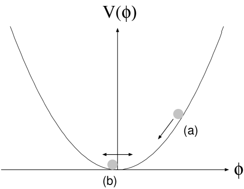
Figure 2.1: Classical Evolution of Scalar Field

Classical evolution of a scalar field, $\phi$, in a potential, $V(\phi)$. (a) $\phi$ rolls down on $V(\phi)$ slowly, driving the universe to expand exponentially. (b) $\phi$ oscillates rapidly about $\phi=0$, terminating inflation; it then decays into particles and radiation because of interactions, reheating the universe.

2.2 Quantum Fluctuations

Inflation predicts emergence of quantum fluctuations in early universe. As soon as the fluctuations emerge from a vacuum, the exponential expansion stretches the proper wavelength of the fluctuations out of the Hubble-horizon scale, $H^{-1}$. After leaving the horizon, the fluctuation amplitude does not change in time; on the contrary, it stays constant in time with characteristic r.m.s. amplitude, $\left|\phi\right|_{\rm rms}\sim H/(2\pi)$.

After inflation, as the universe decelerates, the fluctuations reenter the Hubble horizon, seeding matter and radiation fluctuations in the universe. Figure 2.2 summarizes the evolution of characteristic length scales: the Hubble-horizon scale ($H^{-1}$), the COBE DMR-scale fluctuation wavelength, and the galaxy-scale fluctuation wavelength.

We estimate $H^{-1}$ during inflation as follows. The scalar-field fluctuations produce CMB fluctuations of order $H/m_{\rm pl}$. Using the DMR measurement (Smo92), $\Delta T/T\sim 10^{-5}$, we obtain $H\sim 10^{-5}m_{\rm pl}$, or $H^{-1}\sim 10^{5}m_{\rm pl}^{-1}\sim 10^{-28}~{}{\rm cm}$. Since $H^{-1}$ stays nearly constant in time during inflation, this value represents the horizon scale throughout inflation approximately. After inflation, $H^{-1}$ grows as $H^{-1}(a)\propto a^{2}$ in the radiation era, and $\propto a^{3/2}$ in the matter era.

DMR probes a present-day fluctuation wavelength on the order of $3~{}{\rm Gpc}\sim 10^{28}~{}{\rm cm}$. By comparing the reheating temperature, $\sim 10^{27-29}~{}{\rm K}$, with the present-day CMB temperature, $2.73~{}{\rm K}$, one finds that the universe has expanded by a factor of $a_{0}/a_{\rm rh}\sim 3\times 10^{26-28}$ since the reheating; thus, the DMR scale corresponds to a proper wavelength of $0.3-30$ cm at the reheating epoch (the number could be more uncertain). Here, $a_{0}$ is the present-day scale factor, while $a_{\rm rh}$ is the reheating epoch.

The galaxy-scale fluctuations have the linear comoving wavelength on the order of $1~{}{\rm Mpc}\sim 3\times 10^{24}~{}{\rm cm}$. The galaxy-scale fluctuations have left the horizon later than the DMR-scale fluctuations: $a_{\rm rh}/a_{\rm gal}\sim 10^{25}$, while $a_{\rm rh}/a_{\rm dmr}\sim 10^{28}$. Here, $a_{\rm gal}$ and $a_{\rm dmr}$ are the scale factors at which the galaxy- and DMR-scale fluctuations leave the horizon, respectively.

These ratios are often calculated with $e$-folding numbers, $N\equiv\ln(a_{\rm rh}/a)$. For the galaxy- and DMR-scale fluctuations, we have $N_{\rm gal}=\ln(a_{\rm rh}/a_{\rm gal})\sim 58$, and $N_{\rm dmr}=\ln(a_{\rm rh}/a_{\rm dmr})\sim 64$. Moreover, using equation (2.1), we obtain $t_{\rm gal}-t_{\rm dmr}=H^{-1}(N_{\rm dmr}-N_{\rm gal})\sim 10^{-38}~{}{\rm s}$; thus, inflation generates the fluctuations on the DMR scales down to the galaxy scales almost instantaneously.

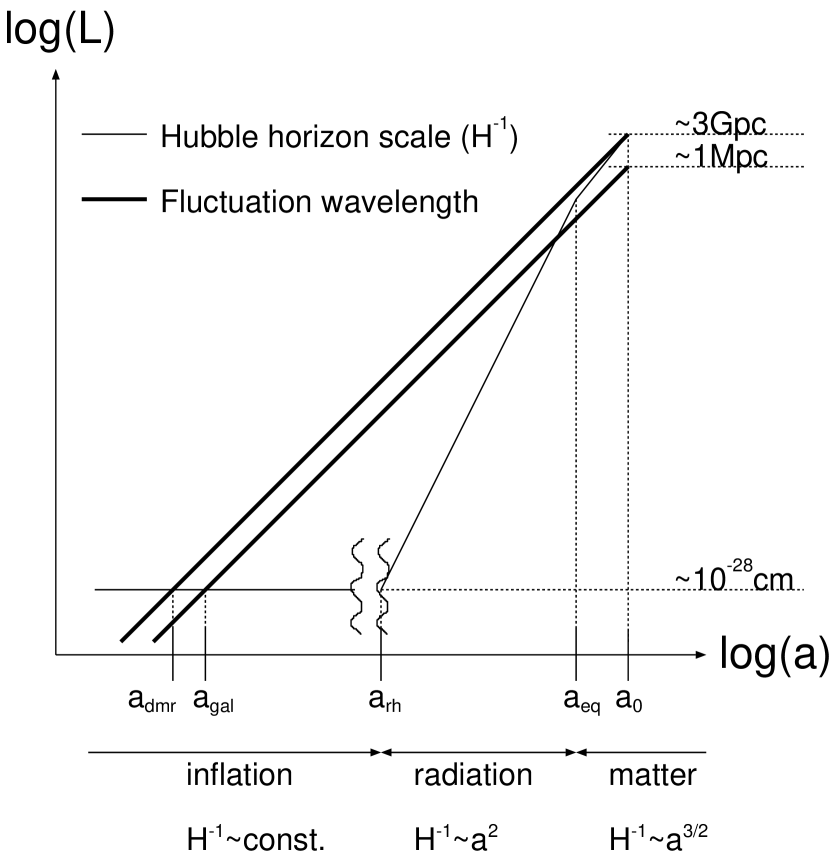
Figure 2.2: Physical Length Scales in Cosmic Evolution

Representative physical length-scale evolution in the cosmic history. The thick lines draw the evolution of fluctuation wavelengths, $2\pi a/k$, while the thin line draws the evolution of the Hubble-horizon scale, $H^{-1}(a)$, where $a$ is the expansion scale factor. $H^{-1}(a)$ stays constant during inflation, grows as $a^{2}$ in the radiation era, and grows as $a^{3/2}$ in the matter era. There are characteristic scale factors: $a_{0}$ is the present-day, $a_{\rm eq}$ is the matter-radiation equality, and $a_{\rm rh}$ is the reheating epoch. The DMR-scale fluctuations leave the horizon at $a_{\rm dmr}$, while the galaxy-scale fluctuations leave at $a_{\rm gal}$. These scale factors are related to each other roughly as follows: $a_{0}/a_{\rm eq}\sim 10^{4}$, $a_{\rm eq}/a_{\rm rh}\sim 10^{24}$, $a_{\rm rh}/a_{\rm gal}\sim 10^{25}$ ($e^{58}$), and $a_{\rm rh}/a_{\rm dmr}\sim 10^{28}$ ($e^{64}$).

2.2.1 Quantization in de Sitter spacetime

A basic idea behind quantum-fluctuation generation in inflation is well described by the second quantization of a massive-free scalar field in unperturbed de Sitter spacetime, for which $a(t)=a_{0}e^{H(t-t_{0})}$ with $H$ independent of $t$. In this system, the problem is exactly solvable, and finite mass captures an essential point of generating a “tilted” fluctuation spectrum, as we will show in the next subsection. In this subsection, we describe the quantization procedure in de Sitter spacetime, following BD82.

Quantization in curved spacetime is generally complicated, as there is no unique vacuum state to define a ground state of quanta, even for inertial observers who detect no particles in the Minkowski vacuum (the vacuum state for the quantum field theory in Minkowski spacetime). Fortunately, in the spatially-flat Robertson-Walker metric, there is a prescription for quantization, largely because of the metric being conformal to the Minkowski metric, $g_{\mu\nu}=a^{2}\eta_{\mu\nu}$, or more specifically

$$ds^{2}=-dt^{2}+a^{2}(t)\delta_{ij}dx^{i}dx^{j}=a^{2}(\tau)\left(-d\tau^{2}+\delta_{ij}dx^{i}dx^{j}\right),$$ (2.3)

where $\tau\equiv\int^{t}a^{-1}(t^{\prime})dt^{\prime}$ is called the conformal time. In this metric, there is a reasonable vacuum state for particles whose comoving frequencies, $\omega_{k}$, are higher than the conformal expansion rate, $d\ln a/d\tau$. We should differ the conformal expansion rate, $d\ln a/d\tau$, from the expansion rate, $H=d\ln a/dt$. They are related through $d\ln a/d\tau=aH$. In de Sitter spacetime, we obtain

$$\tau=\tau_{0}+\frac{1-\exp\left[-H(t-t_{0})\right]}{a_{0}H}=\left(\tau_{0}+\frac{1}{a_{0}H}\right)-\frac{1}{a(\tau)H}.$$ (2.4)

For simplicity, we set the first term vanishing, so that $\tau=-\left[a(\tau)H\right]^{-1}$; thus, $\tau$ lies in $-\infty<\tau<0$ for $-\infty<t<\infty$ ($0<a<\infty$). From now on, we will use dots for conformal-time derivatives: $\dot{x}\equiv\partial x/\partial\tau$.

We start quantizing a scalar field, $\phi({\mathbf{x}},\tau)$, by expanding it into creation, $\hat{a}^{\dagger}_{\mathbf{k}}$, and annihilation, $\hat{a}_{\mathbf{k}}$, operators, which satisfy the commutation relation, $\left[\hat{a}_{\mathbf{k}},\hat{a}^{\dagger}_{{\mathbf{k}}^{\prime}}\right]=\delta^{(3)}({\mathbf{k}}-{\mathbf{k}}^{\prime})$. We have

$$\phi({\mathbf{x}},\tau)=\int\frac{d^{3}{\mathbf{k}}}{(2\pi)^{3/2}}\left[\hat{a}_{\mathbf{k}}\varphi_{k}(\tau)e^{i{\mathbf{k}}\cdot{\mathbf{x}}}+\hat{a}^{\dagger}_{\mathbf{k}}\varphi^{*}_{k}(\tau)e^{-i{\mathbf{k}}\cdot{\mathbf{x}}}\right].$$ (2.5)

The canonical commutation relation between $\phi$ and the conjugate momentum, $\pi_{\phi}=a^{2}(\tau)\dot{\phi}$:

$$\left[\phi({\mathbf{x}},\tau),\pi_{\phi}({\mathbf{x}}^{\prime},\tau)\right]=a^{2}(\tau)\left[\phi({\mathbf{x}},\tau),\dot{\phi}({\mathbf{x}}^{\prime},\tau)\right]=i\delta^{(3)}({\mathbf{x}}-{\mathbf{x}}^{\prime}),$$ (2.6)

gives a normalization condition on $\varphi_{k}(\tau)$, $a^{2}\left(\varphi_{k}\dot{\varphi}^{*}_{k}-\varphi^{*}_{k}\dot{\varphi}_{k}\right)=i$.

The normalization condition motivates our using a new mode function given by $\chi_{k}\equiv a\varphi_{k}$, which satisfies a new normalization condition, $\chi_{k}\dot{\chi}^{*}_{k}-\chi^{*}_{k}\dot{\chi}_{k}=i$. If $\chi_{k}$ has a positive frequency mode with respect to the conformal timelike Killing vector ($\partial/\partial\tau$ for our metric), i.e., $\dot{\chi}_{k}=-i\omega_{k}\chi_{k}$, then the condition gives $\chi_{k}(\tau)=(2\omega_{k})^{-1/2}e^{-i\omega_{k}\tau}$, a ground state in the Minkowski vacuum. Since $\chi_{k}$ gives the closest analogy to the Minkowski vacuum state, we will use $\chi_{k}$ more frequently than $\varphi_{k}$.

The Klein–Gordon equation for a massive-free scalar field, $g^{\alpha\beta}\phi_{,\alpha;\beta}=m^{2}\phi^{2}$, gives equation of motion for $\chi_{k}(\tau)$,

$$\ddot{\chi}_{k}(\tau)+\left[k^{2}+m^{2}_{\chi}(\tau)\right]\chi_{k}(\tau)=0,$$ (2.7)

where $m^{2}_{\chi}(\tau)$ is the time-dependent effective mass,

$$m_{\chi}^{2}(\tau)\equiv(m^{2}-2H^{2})a^{2}(\tau)=m^{2}a^{2}(\tau)-\frac{2}{\tau^{2}}.$$ (2.8)

We thus find that the Hubble parameter effectively reduces $m^{2}$ by $2H^{2}$. This time-dependent, negative contribution to $m_{\chi}^{2}(\tau)$ is the effect of de Sitter spacetime, which is not Minkowski but curved.

Fortunately, there is an exact solution to the Klein–Gordon equation (2.7):

$$\chi_{k}(\tau)=\sqrt{-\tau}\left[C_{1}H^{(1)}_{\nu}\left(-k\tau\right)+C_{2}H^{(2)}_{\nu}\left(-k\tau\right)\right],$$ (2.9)

where $C_{1}$ and $C_{2}$ are integration constants, and $\nu^{2}=9/4-{m^{2}}/{H^{2}}$. $H^{(1)}_{\nu}(x)$ is a Hankel function of the first kind; $H^{(2)}_{\nu}(x)=\left[H^{(1)}_{\nu}(x)\right]^{*}$. We have negative sign in front of $\tau$ to recall that $\tau$ lies in $-\infty<\tau<0$.

How do we determine the integration constants, $C_{1}$ and $C_{2}$? In other words, how do we normalize our mode function properly? Since we know how to quantize a scalar field in the Minkowski vacuum, we should find a mode function that matches the Minkowski positive frequency mode, $\chi_{k}(\tau)=(2\omega_{k})^{-1/2}e^{-i\omega_{k}\tau}$; however, we cannot find an unique positive frequency mode valid throughout inflation, as the time-dependent spacetime creates particles.

Instead, we define a vacuum state in the in state, the remote past, $\tau\rightarrow-\infty$. Using an asymptotic form of the Hankel function,

$$H^{(1)}_{\nu}(x\gg 1)\approx\sqrt{\frac{2}{\pi x}}\exp\left[i\left(x-\nu\frac{\pi}{2}-\frac{\pi}{4}\right)\right],$$ (2.10)

we obtain $\chi_{k}$ in the in state ($\tau\rightarrow-\infty$) from equation (2.9),

$$\chi_{k}(\tau\rightarrow-\infty)\longrightarrow\sqrt{\frac{2}{\pi k}}\left(C_{1}e^{-ik\tau}+C_{2}e^{ik\tau}\right).$$ (2.11)

Here, we have neglected the contribution from $m^{2}/H^{2}$ compared with $-k\tau$ in the exponent. The second term has a negative frequency, so that $C_{2}=0$. The first term with $C_{1}=\sqrt{\pi}/2$ gives $\chi_{k}(\tau)=(2k)^{-1/2}e^{-ik\tau}$, the Minkowski positive frequency mode with $\omega_{k}=k$, and thus in the in state, the solution describes a ground state of a massless field in the Minkowski vacuum.

Using the solution for $\chi_{k}(\tau)$, we obtain a solution for $\varphi_{k}(\tau)$,

$$\varphi_{k}(\tau)=\frac{\sqrt{-\pi\tau}}{2a(\tau)}H^{(1)}_{\nu}\left(-k\tau\right),$$ (2.12)

and $\phi({\mathbf{x}},\tau)$ becomes

$$\phi({\mathbf{x}},\tau)=\frac{\sqrt{-\pi\tau}}{2a(\tau)}\int\frac{d^{3}{\mathbf{k}}}{(2\pi)^{3/2}}\left[\hat{a}_{\mathbf{k}}H^{(1)}_{\nu}\left(-k\tau\right)e^{i{\mathbf{k}}\cdot{\mathbf{x}}}+\hat{a}^{\dagger}_{\mathbf{k}}H^{(2)}_{\nu}\left(-k\tau\right)e^{-i{\mathbf{k}}\cdot{\mathbf{x}}}\right].$$ (2.13)

Since all the $k$ modes in the integral are independent of each other, the nearly infinite sum of those modes makes $\phi$ obey Gaussian statistics almost exactly, because of the central limit theorem; thus, the two-point statistics specify all the statistical properties of $\phi$. This is a generic property of the ground-state quantum fluctuations.

The annihilation operator, $\hat{a}_{\mathbf{k}}$, annihilates the vacuum state defined in the in state: $\left.\left.\hat{a}_{\mathbf{k}}\right|0_{\rm in}\right>=0$. In this vacuum, we calculate amplitude of ground-state $\phi$ fluctuations as

$$\left<0_{\rm in}\left|\phi^{\dagger}({\mathbf{x}},\tau)\phi({\mathbf{x}},\tau)\right|0_{\rm in}\right>=\int_{0}^{\infty}\frac{k^{2}dk}{2\pi^{2}}\left|\varphi_{k}(\tau)\right|^{2}=\frac{-\tau}{8\pi a^{2}(\tau)}\int_{0}^{\infty}k^{2}dk\left|H_{\nu}^{(1)}(-k\tau)\right|^{2}.$$ (2.14)

Since we probe a limited range of $k$ observationally, we also use the fluctuation spectrum in a logarithmic $k$ range, $\Delta^{2}(k)$, which represents variance of fluctuations at a given comoving wavelength $2\pi k^{-1}$,

$$\Delta^{2}_{\phi}(k)\equiv\frac{k^{3}}{2\pi^{2}}\left|\varphi_{k}(\tau)\right|^{2}=\frac{-k^{3}\tau\left|H_{\nu}^{(1)}(-k\tau)\right|^{2}}{8\pi a^{2}(\tau)}=\frac{H^{2}}{8\pi}(-k\tau)^{3}\left|H_{\nu}^{(1)}(-k\tau)\right|^{2},$$ (2.15)

where we have used $a(\tau)=-(H\tau)^{-1}$ in the last equality. Let us recall that $\nu^{2}=9/4-{m^{2}}/{H^{2}}$, and $\tau$ lies in $-\infty<\tau<0$.

Here, we have the quantization of $\phi$ completed, and formally calculated the fluctuation spectrum. These results are exact, and valid on all scales. In the next subsection, we study the solution on super-horizon scales, where inflation produces observationally relevant fluctuations.

2.2.2 Scale-invariant fluctuations on super-horizon scales

Equation (2.13) describes a quantum massive-free scalar field, $\phi$, in the unperturbed de Sitter spacetime on all scales. As the universe expands exponentially, $-k\tau=k/(aH)$ quickly becomes very small; the mode leaves the Hubble-horizon scale, $H^{-1}$. Figure 2.2 shows that the fluctuations on the observationally relevant scales should have left the horizon during inflation. Hence, the behavior of $\phi$ on super-horizon scales is practically important. In this subsection, we study the $\phi$ fluctuation spectrum on super-horizon scales.

In equation (2.15), using an asymptotic form of the Hankel function,

$$H^{(1)}_{\nu}(x\ll 1)\approx-i\frac{\Gamma(\nu)}{\pi}\left(\frac{x}{2}\right)^{-\nu},$$ (2.16)

we obtain the $\phi$ fluctuation spectrum on super-horizon scales,

$$\Delta^{2}_{\phi}(k)\approx\left(\frac{H}{2\pi}\right)^{2}2^{2\nu-3}\left[\frac{\Gamma(\nu)}{\Gamma(3/2)}\right]^{2}\left(\frac{k}{aH}\right)^{3-2\nu},$$ (2.17)

where $\nu^{2}=9/4-m^{2}/H^{2}$. We have used $\tau=-(aH)^{-1}$ and $\pi=\Gamma^{2}(1/2)=4\Gamma^{2}(3/2)$.

One finds that $\nu=3/2$ is a special point, for which the spectrum is independent of $k$, i.e., scale invariant, $\Delta^{2}_{\phi}(k)=H^{2}/(2\pi)^{2}$. This happens when we assume $m^{2}/H^{2}\ll 1$, and thus $\nu=3/2-m^{2}/(3H^{2})+{\cal O}(m^{4}/H^{4})$, which gives

$$\Delta^{2}_{\phi}(k)\approx\left(\frac{H}{2\pi}\right)^{2}\left(\frac{k}{aH}\right)^{2m^{2}/(3H^{2})},$$ (2.18)

or the spectral index,

$$\frac{d\ln\Delta^{2}_{\phi}}{d\ln k}=\frac{2m^{2}}{3H^{2}}.$$ (2.19)

Since $m^{2}\ll H^{2}$, the spectrum is almost scale invariant, giving the $\phi$ fluctuations characteristic r.m.s. amplitude, $\left|\phi\right|_{\rm rms}=H/(2\pi)$. Finite mass makes the spectrum slightly “blue”, the power of $k$ being positive.

The above assumption, $m^{2}\ll H^{2}$, offers long-lasting inflation that makes the observable universe flat and homogeneous; otherwise, $\phi$ rolls down to a potential minimum too quickly, terminating inflation too early. In the inflationary regime, the Friedmann equation gives

$$\frac{m^{2}}{H^{2}}=\frac{3}{4\pi}\frac{m_{\rm pl}^{2}}{\phi^{2}}\sim 10^{-2}.$$ (2.20)

Hence, for a massive-free scalar field to drive inflation, the mass cannot be comparable to the Hubble parameter, and the fluctuation spectrum is almost exactly scale invariant.

The argument until now has assumed the exact de Sitter spacetime in which $H$ is constant in time, and neglected perturbations in the metric. As a result, we have obtained a blue spectrum whose spectral index is $0<2m^{2}/3H^{2}\ll 1$. In realistic inflation models, however, none of the above assumptions apply: $H$ decreases slowly in time, and the metric is perturbed. In the next subsection, we will show that both the effects give a tilted “red” spectrum, for which the power of $k$ is negative of order $-10^{-2}$. Figure 2.3 sketches what blue, scale-invariant, and red spectra look like.

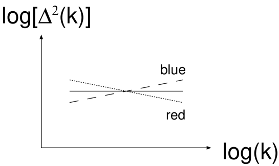
Figure 2.3: Color of Spectrum

A sketch of the fluctuation spectrum, $\Delta^{2}(k)$, which represents the fluctuation power in a logarithmic $k$ range. The solid line plots a scale-invariant spectrum, the dotted line plots a “red” spectrum whose spectral index is negative, and the dashed line plots a “blue” spectrum whose spectral index is positive.

2.2.3 Tilted “red” spectrum

If $H$ decreases in time, and the metric is linearly perturbed, a scalar field acquires a negative effective mass-squared, $\Delta m^{2}<0$. It also modifies the mass of $\chi_{k}$, $m_{\chi}(\tau)$ (Eq.(2.8)), as

$$m_{\chi}^{2}(\tau)\longrightarrow\left(m^{2}+\Delta m^{2}\right)a^{2}(\tau)-\frac{2}{\tau^{2}}.$$ (2.21)

We thus expect that $\Delta m^{2}$ modifies the fluctuation spectral index, for the mass determines the spectral index through equation (2.19). This parameterization, $\Delta m^{2}$, may be useful to understand what physical effect is responsible for the spectral index.

How large is $\Delta m^{2}$? The derivation of $\Delta m^{2}$ is quite involved, but MFB92 show that the exact form of $m_{\chi}^{2}(\tau)$

$$m_{\chi}^{2}(\tau)=-\frac{H}{\dot{\phi}}\frac{d^{2}({\dot{\phi}}/{H})}{d\tau^{2}}\approx\left(\frac{d^{2}V}{d\phi^{2}}+9\frac{dH}{dt}\right)a^{2}(\tau)-\frac{2}{\tau^{2}}=m^{2}_{\rm eff}\hskip 0.4pta^{2}(\tau)-\frac{2}{\tau^{2}}.$$ (2.22)

Here, since $H$ and $\phi$ change in time $t$ only very slowly, we have retained the terms on the order of $-dH/dt=4\pi m_{\rm pl}^{-2}(d\phi/dt)^{2}$ or larger. This approximation is called the slow-roll approximation, and we evaluate the approximation explicitly in appendix LABEL:app:slowroll. For a massive-free field, $V(\phi)=m^{2}\phi^{2}/2$, by comparing equation (2.22) with (2.21), we find $\Delta m^{2}=9dH/dt<0$. One can show that the 3 of the 9 comes from the effect of $H$ changing in time, and the 6 comes from the effect of the metric perturbations.

By using the first-order slow-roll approximation, we obtain a relation between $dH/dt$ and the potential slope, $dV/d\phi$, $dH/dt\approx-\frac{1}{6V}(dV/d\phi)^{2}=-\frac{1}{3}m^{2}$. It thus follows that the total effective mass-squared becomes negative, $m^{2}_{\rm eff}=m^{2}+\Delta m^{2}\approx-2m^{2}<0$, and we have a “red” spectrum or a negative spectral index,

$$\frac{d\ln\Delta^{2}_{\phi}}{d\ln k}=\frac{2m^{2}_{\rm eff}}{3H^{2}}\approx-\frac{4m^{2}}{3H^{2}}<0.$$ (2.23)

Let us summarize what has made the spectral index negative. The spectral index is determined by the mass, or the effective mass, of a scalar field. In inflation, the intrinsic mass, $m^{2}$, is over-compensated by the induced mass from gravitational effects, $\Delta m^{2}$, which is negative: $m^{2}+\Delta m^{2}<0$. As a result, the fluctuation spectrum becomes “red”. Actually, any power-law potential of the form $V(\phi)=A\phi^{n}$ with $A$ positive gives a negative $m_{\rm eff}^{2}$ through $m^{2}_{\rm eff}=-(1+n/2)nA\phi^{n-2}$. Here, we have used $dH/dt\approx-\frac{1}{6V}(dV/d\phi)^{2}=-\frac{1}{6}n^{2}A\phi^{n-2}$.

For a generic scalar field with an arbitrary potential, we find

$$m^{2}_{\rm eff}=\frac{d^{2}V}{d\phi^{2}}+9\frac{dH}{dt}=6\frac{dH}{dt}-3H\frac{d^{2}\phi/dt^{2}}{d\phi/dt},$$ (2.24)

and the spectral index

$$\frac{d\ln\Delta^{2}_{\phi}}{d\ln k}=4\frac{dH/dt}{H^{2}}-2\frac{d^{2}\phi/dt^{2}}{H(d\phi/dt)},$$ (2.25)

which agrees with LL92.

CMB experiments have shown that a scale-invariant fluctuation spectrum fits the data well (Boom00; Maxima00). Combining all the CMB experiments to date, WTZ01 show that a slightly red spectrum, the power of $k$ being $\sim-0.07$, fits the data even better, while the error of the fit is still of order $0.1$. Accurate measurement of the spectral index constrains the shape of $V(\phi)$ through equation (2.25), as $V(\phi)$ determines the time variation of $H$ and $\phi$; thus, it potentially discriminates between different inflation models.

Although the CMB experiments almost exclude possibility of the massive-free scalar field with sizable $m^{2}/H^{2}\sim 1$ dominating the matter and radiation fluctuations in the universe (in terms of the spectrum index), the field may produce some of the fluctuations that are non-Gaussian. In this case, $\phi$ does not drive inflation, so that $m^{2}$ can be comparable to $H^{2}$; the field rolls down to a potential minimum quickly, and oscillates about the minimum, producing non-Gaussian isocurvature density fluctuations, $\delta\rho\propto\phi^{2}$ (LM97). Even if the isocurvature fluctuations are sub-dominant in the universe, they could produce non-Gaussian temperature fluctuations in CMB. Measuring non-Gaussianity in CMB thus potentially probes particle physics in inflation.

2.2.4 Emergence of classical fluctuations

Until now, we have considered generation of quantum fluctuations in inflation, and derived a fluctuation spectrum on super-horizon scales. We then expect that the fluctuations seed observed CMB anisotropies and large-scale structures in the universe; but, how? Inflation generates quantum fluctuations, not classical fluctuations. How can the quantum fluctuations make classical objects like galaxies seen today?

Generation of classical fluctuations, or quantum-to-classical transition of fluctuations, during inflation, has been in debate (CH95; Matacz97a; Matacz97b; KPS98). In this subsection, we describe a possible mechanism to produce classical fluctuations in inflation. Our approach is partly close to KPS98.

A basic idea behind our classical-to-quantum transition mechanism is to approximate a field, $\phi$ (Eq.(2.5)), with the sum of the long-wavelength (super-horizon) modes and the short-wavelength (sub-horizon) modes. This mode separation is unique, as the comoving Hubble-horizon scale, $(aH)^{-1}$, has been a characteristic length scale in the solutions for mode functions, $\varphi_{k}(\tau)$ (Eq.(2.12)).

In the super-horizon limit, $k\ll aH$, equations (2.12) and (2.16) give $\varphi_{k\ll aH}^{*}=-\varphi_{k\ll aH}$. Using this in equation (2.5), we obtain

$$\phi({\mathbf{x}},\tau) \approx \int_{k<aH}d^{3}{\mathbf{k}}\left(\hat{a}_{\mathbf{k}}-\hat{a}^{\dagger}_{-{\mathbf{k}}}\right)\varphi_{k\ll aH}(\tau)e^{i{\mathbf{k}}\cdot{\mathbf{x}}}$$ (2.26)

$$+a^{-1}(\tau)\int_{k>aH}\frac{d^{3}{\mathbf{k}}}{(2\pi)^{3/2}\sqrt{2k}}\left(\hat{a}_{\mathbf{k}}e^{i{\mathbf{k}}\cdot{\mathbf{x}}-ik\tau}+\hat{a}^{\dagger}_{\mathbf{k}}e^{-i{\mathbf{k}}\cdot{\mathbf{x}}+ik\tau}\right).$$

We name the first term $\phi_{\rm CL}$, the second term $\phi_{\rm QM}$. The corresponding conjugate momenta are $\pi_{\rm CL}=a^{2}\dot{\phi}_{\rm CL}$ and $\pi_{\rm QM}=a^{2}\dot{\phi}_{\rm QM}$, respectively. The first term, $\phi_{\rm CL}$, becomes just the Fourier transform, while the second term, $\phi_{\rm QM}$, becomes an ordinary ground state in the Minkowski vacuum except for $a^{-1}(\tau)$ in the front. To see what happens to these terms in the context of the quantum field theory, we calculate the canonical commutation relations of $\phi_{\rm CL}$ and $\phi_{\rm QM}$.

For $\phi_{\rm QM}$, we find

$$\left[\phi_{\rm QM}({\mathbf{x}},\tau),\pi_{\rm QM}({\mathbf{x}}^{\prime},\tau)\right]=i\int_{k>aH}\frac{d^{3}{\mathbf{k}}}{(2\pi)^{3}}e^{i{\mathbf{k}}\cdot({\mathbf{x}}-{\mathbf{x}}^{\prime})}=i\delta^{(3)}({\mathbf{x}}-{\mathbf{x}}^{\prime})$$ (2.27)

for $\left|{\mathbf{x}}-{\mathbf{x}}^{\prime}\right|<(aH)^{-1}$; thus, $\phi_{\rm QM}$ is a quantum field inside the horizon, and $a\phi_{\rm QM}$ is identical to a quantum field in the Minkowski vacuum. For $\phi_{\rm CL}$, we find the commutation relation vanishing,

$$\left[\phi_{\rm CL}({\mathbf{x}},\tau),\pi_{\rm CL}({\mathbf{x}}^{\prime},\tau)\right]=0;$$ (2.28)

thus, $\phi_{\rm CL}$ is no longer a quantum field, but a classical field. In other words, once smoothing out the fluctuations inside the horizon, we are left with the classical fluctuations. Notice that there has been no explicit decoherence mechanism in the system. The exact solution to the Klein–Gordon equation in the exact de Sitter spacetime naturally yields the classical fluctuations on super-horizon scales.

Without smoothing out the sub-horizon fluctuations, however, $\phi$ remains quantum. The commutation relation of $\phi$ (Eq.(2.6)) is exact as long as all the $k$ modes equally contribute to $\phi$. If nothing happens to the sub-horizon fluctuations, then the quantum, not classical, fluctuations will reenter the horizon after inflation. Yet, practically speaking, this argument may not be relevant for our actual observations because of the following reason. Consider a fluctuation wavelength just leaving the horizon at the end of inflation, at which the proper horizon size is $H^{-1}\sim 10^{-28}~{}{\rm cm}$. As the universe has expanded by a factor of order $10^{27}$ since the end of inflation, we may find the fluctuation wavelength to be $\sim 0.1~{}{\rm cm}$ in the present universe. Now we ask: “does this-size fluctuation affects classicality of galaxy-scale fluctuations?” We may answer “no”, if we assume that these substantially different-scale fluctuations have undergone different physics; if so, quantum coherence should have disappeared.

Even right after inflation, the super-horizon modes and the sub-horizon modes have undergone different physics. At the end of inflation, the reheating begins, and scalar fields decay into particles and radiation, thermalizing the universe. By causality, the thermalization process occurs only inside the horizon; thus, the reheating affects the sub-horizon fluctuations differently from the super-horizon fluctuations, breaking quantum nature of $\phi$. In other words, in equation (2.26), the second term may have disappeared during the reheating, while the first term may remain unaffected. As a result, the reheating effectively smoothes out the sub-horizon scale fluctuations, and makes a quantum-to-classical transition possible.

2.3 Linear Perturbation Theory in Inflation

In the previous section, we have followed generation of scalar-field fluctuations in the unperturbed de Sitter spacetime, i.e., no perturbations in the metric. Scalar-field fluctuations, however, perturb the stress-energy tensor, and produce metric perturbations. Since the metric perturbations regulate the matter and radiation fluctuations that we observe today, we must include the metric perturbations in the analysis, and follow the evolution. In this section, we explore the linear perturbation theory in inflation, which includes perturbations to the metric and a scalar field. Our notation follows Bardeen80.

We use a linearly perturbed conformal Robertson–Walker metric of the form,

$$ds^{2}=a^{2}(\tau)\left\{-(1+2AQ)d\tau^{2}-2BQ_{i}d\tau dx^{i}+\left[\left(1+2H_{\rm L}Q\right)\delta_{ij}+2H_{\rm T}Q_{ij}\right]dx^{i}dx^{j}\right\}.$$ (2.29)

Here, all the metric perturbations, $A$, $B$, $H_{\rm L}$, and $H_{\rm T}$, are $\ll 1$, and functions of $\tau$. The spatial coordinate dependence of the perturbations is described by the scalar harmonic eigenfunctions, $Q$, $Q_{i}$, and $Q_{ij}$, that satisfy $\delta^{ij}Q_{,ij}=-k^{2}Q$, $Q_{i}=-k^{-1}Q_{,i}$, and $Q_{ij}=k^{-2}Q_{,ij}+\frac{1}{3}\delta_{ij}Q$. Note that $Q_{ij}$ is traceless: $\delta^{ij}Q_{ij}=0$. KS84 use different symbols, $Y$, $Y_{i}$, and $Y_{ij}$, for $Q$, $Q_{i}$, and $Q_{ij}$, respectively.

The four metric-perturbation variables are not entirely free, but some of which should be fixed to fix our coordinate system before we analyze the perturbations. The choice of coordinate system is often called the choice of gauge, or the gauge transformation; we will describe it later.

2.3.1 Fluid representation of scalar field

The metric perturbations enter into the stress-energy tensor perturbations, $\delta T^{\mu}_{\nu}$. We expand a scalar field into its homogeneous mean field, $\phi(\tau)$, and fluctuations about the mean, $\delta\phi(\tau)Q({\mathbf{x}})$. The energy density and pressure fluctuations are given by

$$\delta\rho_{\phi}Q \equiv -\delta T^{0}_{0}=\left[a^{-2}\left(\dot{\phi}\delta\dot{\phi}-A\dot{\phi}^{2}\right)+V_{,\phi}\delta\phi\right]Q,$$ (2.30)

$$\delta p_{\phi}Q \equiv \frac{\delta T^{k}_{k}}{3}=\left[a^{-2}\left(\dot{\phi}\delta\dot{\phi}-A\dot{\phi}^{2}\right)-V_{,\phi}\delta\phi\right]Q.$$ (2.31)

The energy flux, $T^{0}_{i}$, gives the velocity field, $v_{\phi}Q_{i}$,

$$\left(\rho_{\phi}+p_{\phi}\right)\left(v_{\phi}-B\right)Q_{i}\equiv T^{0}_{i}=\left(\frac{\dot{\phi}}{a^{2}}k\delta\phi\right)Q_{i}.$$ (2.32)

Using $\rho_{\phi}+p_{\phi}=a^{-2}\dot{\phi}^{2}$, we obtain $v_{\phi}-B=k\dot{\phi}^{-1}\delta\phi$; thus, $\delta\phi$ is directly responsible for the fluid’s peculiar motion. The anisotropic stress, $T^{i}_{j}-p_{\phi}\delta^{i}_{j}$, is a second-order perturbation variable for a scalar field, being negligible.

When we choose our coordinate system so as $B\equiv v_{\phi}$ (a fluid element is comoving with the origin of the spatial coordinate), we have $\delta\phi$ vanishing, $\delta\phi\equiv 0$. This coordinate is called the comoving gauge, and we write the scalar-field fluctuations in this gauge as $\delta\phi_{\rm com}\equiv 0$.

Since we have only one degree of freedom, a scalar field, in the system, $\delta\rho_{\phi}$, $\delta p_{\phi}$, and $v_{\phi}$ are not independent of each other. Nevertheless, this fluid representation is useful, as the cosmological linear perturbation theory has been developed as the general relativistic fluid dynamics. We can plague these fluid variables into the well-established general relativistic fluid equations, and see what happens to the metric perturbations. While we do not use those fluid equations explicitly in the following, but solve equation of motion for a scalar field (Klein–Gordon equation) directly, the fluid equations give the same answer.

2.3.2 Gauge-invariant perturbations

In the previous subsection, we have seen that scalar-field fluctuations vanish in the comoving gauge in which $B\equiv v_{\phi}$; thus, a choice of gauge defines perturbations. For the scalar-type perturbations that we are considering, the gauge transformation is

$$\tau \longrightarrow \tau^{\prime}=\tau+T(\tau)Q({\mathbf{x}}),$$ (2.33)

$$x^{i} \longrightarrow x^{\prime}{}^{i}=x^{i}+L(\tau)Q_{i}({\mathbf{x}}),$$ (2.34)

where $T$ and $L$ are $\ll 1$. Accordingly, scalar-field fluctuations, $\delta\phi$, transform as

$$\delta\phi(\tau)\longrightarrow\widetilde{\delta\phi}(\tau^{\prime})=\delta\phi(\tau)-\dot{\phi}(\tau)T(\tau).$$ (2.35)

Hence, if we choose $T=\dot{\phi}^{-1}\delta\phi$, then we obtain $\widetilde{\delta\phi}=0$. This choice of $T$ defines the comoving gauge, $\delta\phi_{\rm com}=0$. In this way, we find different values for the perturbation variables in different gauges.

So, what gauge should we use? Unfortunately, there is no answer to the question: “what gauge should we use?”. Although there is no best gauge in the world, depending on a problem that we intend to solve, we may find that one gauge is more useful than the other, or vice versa. As long as we fix the gauge uniquely, and understand what gauge we are working on clearly, no problems occur.

In practice, however, problems occur when one author understands its own gauge, but does not understand the other author’s gauge. Since there is no best gauge in the world, different authors may use different gauges, and may disagree with each other because of their misunderstanding of the gauges. In other words, one author’s calculation on amplitude of $\delta\phi$ may disagree with the other’s calculation, if they are using different gauges. The author using the comoving gauge sees $\delta\phi=0$, but others may see $\delta\phi\neq 0$.

One way to overcome this undesirable property is to make perturbation variables invariant under the gauge transformation, and let them represent gauge-invariant perturbations. As an example, consider a new perturbation variable (MFB92),

$$u\equiv\delta\phi-\frac{\dot{\phi}}{aH}\left(H_{\rm L}+\frac{1}{3}H_{\rm T}\right).$$ (2.36)

One can prove this variable gauge invariant, $\widetilde{u}=u$, using equation (2.35) and

$$\widetilde{H}_{\rm L}+\frac{1}{3}\widetilde{H}_{\rm T}=H_{\rm L}+\frac{1}{3}H_{\rm T}-aHT.$$ (2.37)

Actually, $H_{\rm L}+\frac{1}{3}H_{\rm T}$ represents perturbations in the intrinsic spatial curvature, ${\cal R}$, as it is the scalar potential of the 3-dimension Ricci scalar: $\delta^{(3)}R=a^{-2}k^{2}{\cal R}Q$, where ${\cal R}\equiv H_{\rm L}+\frac{1}{3}H_{\rm T}$. While $u$ reduces to $\delta\phi$ in the spatially flat gauge (${\cal R}\equiv 0$), or to $-(\dot{\phi}/aH){\cal R}$ in the comoving gauge ($\delta\phi\equiv 0$), its value is invariant under any gauge transformation. Any authors should agree upon the value of $u$.

For the physical interpretation of $u$, we may name $u$ “scalar-field fluctuations in the spatially flat gauge” or “intrinsic spatial curvature perturbations in the comoving gauge”. Either name describes the physical meaning of $u$ correctly. The physical meaning of $u$ depends upon what gauge we are using; however, the most important point is that the value of $u$ is independent of a gauge choice. In this sense, $u$ can be a “common language” among different authors.

BST83 use a similar gauge-invariant variable to $u$,

$$\zeta\equiv-\frac{aH}{\dot{\phi}}u={\cal R}-\frac{aH}{\dot{\phi}}\delta\phi,$$ (2.38)

that reduces to ${\cal R}$ in the comoving gauge, or to $-(aH/\dot{\phi})\delta\phi$ in the spatially flat gauge. This variable helps our perturbation analysis not only because of being gauge invariant, but also being conserved on super-horizon scales throughout the cosmic evolution. We will show this property in the next subsection.

Using gauge invariance of $u$ or $\zeta$, we obtain a relation between $\delta\phi$ in the spatially flat gauge, $\delta\phi_{\rm flat}$, and ${\cal R}$ in the comoving gauge, ${\cal R}_{\rm com}$, as

$${\cal R}_{\rm com}=-\frac{aH}{\dot{\phi}}\delta\phi_{\rm flat}.$$ (2.39)

It is derived from $u_{\rm com}=u_{\rm flat}$, or $\zeta_{\rm com}=\zeta_{\rm flat}$. As we have seen in the previous section, $\delta\phi$ obeys Gaussian statistics to very good accuracy because of the central limit theorem, that is, $\delta\phi$ is the sum of the nearly infinite number of independent modes (Eq.(2.13)). Since ${\cal R}_{\rm com}$ is linearly related to $\delta\phi_{\rm flat}$, ${\cal R}_{\rm com}$ also obeys Gaussian statistics in the linear order; however, as we will show in the next section, non-linear correction to this linear relation makes ${\cal R}_{\rm com}$ weakly non-Gaussian.

The spatial curvature perturbation, ${\cal R}$, is more relevant for the structure formation in the universe than the scalar-field fluctuation, $\delta\phi$, itself, as ${\cal R}$ regulates the matter density and velocity perturbations through the Poisson equation. Actually, ${\cal R}$ reduces to the Newtonian potential inside the horizon. Since the quantum fluctuations generate $\delta\phi$, we expect it to generate ${\cal R}$ through ${\cal R}_{\rm com}=-(aH/\dot{\phi})\delta\phi_{\rm flat}$. This is naively true, but may sound tricky. In the next subsection, we will show how to calculate ${\cal R}$ generated in inflation more rigorously.

2.3.3 Generation of spatial curvature perturbations

To calculate the intrinsic spatial curvature perturbation, ${\cal R}=H_{\rm L}+\frac{1}{3}H_{\rm T}$, that is generated in inflation, we need to track its evolution equation, and figure out how it is related to $\delta\phi$. We will show in this subsection that ${\cal R}$ is actually more than related to $\delta\phi$; it is almost equivalent to $\delta\phi$. We can track the evolution of $\delta\phi$ and ${\cal R}$ simultaneously, using the gauge-invariant variable, $u$ (Eq.(2.36)).

MFB92 show that $au=a\delta\phi-(\dot{\phi}/H){\cal R}$ obeys the same Klein–Gordon equation as we have used in the previous section (Eq.(2.7)),

$$\ddot{\chi}_{k}+\left[k^{2}+m^{2}_{\chi}(\tau)\right]\chi_{k}=0,$$ (2.40)

where $\chi_{k}$ is the mode function that expands $au$ (see Eq.(2.5)). It thus follows that $a\delta\phi$ and $(\dot{\phi}/H){\cal R}$ obey the same equation, and our argument on the quantum-fluctuation generation during inflation in the previous section applies to $u$ as well. $u$ being quantum fluctuations means that it also obeys Gaussian statistics very well because of the central limit theorem (see Eq.(2.13) and the text after equation).

We consider the Klein–Gordon equation for $au$ on super-horizon scales. As equation (2.5), we expand $au$ into the mode functions, $\chi_{k}=a\varphi_{k}$, where $\chi_{k}$ and $\varphi_{k}$ are exactly the same functions that we have used in the previous section.

We give a slightly different expression for the solution, emphasizing its time dependence on super-horizon scales. Taking the long-wavelength limit, $k^{2}\ll m_{\chi}^{2}(\tau)$, and using the exact form of $m^{2}_{\chi}(\tau)$ (Eq.(2.22)) (MFB92), we obtain the Klein–Gordon equation on super-horizon scales,

$$\ddot{\chi}_{k}-\frac{H}{\dot{\phi}}\frac{d^{2}({\dot{\phi}}/{H})}{d\tau^{2}}\chi_{k}=0.$$ (2.41)

There is an exact solution to this equation,

$$\frac{H}{\dot{\phi}}{\chi}_{k}=\frac{aH}{\dot{\phi}}{\varphi}_{k}=C_{1}+C_{2}\int\frac{H^{2}}{\dot{\phi}^{2}}d\tau,$$ (2.42)

where $C_{1}$ and $C_{2}$ are integration constants independent of $\tau$. The second term is a decaying mode as $\int\dot{\phi}^{-2}H^{2}d\tau=\int a^{-3}(d\phi/dt)^{-2}H^{2}dt$, and thus $(H/\dot{\phi}){\chi}_{k}$ remains constant in time on super-horizon scales. This implies that $\zeta=-(aH/\dot{\phi})u$ also remains constant in time on super-horizon scales. Note that $\zeta$ obeys Gaussian statistics in the linear order, as it is related to a Gaussian variable, $u$, linearly; however, as we will show in the next section, non-linear correction to this linear relation makes $\zeta$ weakly non-Gaussian. This statement is equivalent to that we have made on ${\cal R}_{\rm com}$.

The solution obtained here for $\zeta$ is valid throughout the cosmic history regardless of whether a scalar field, radiation, or matter dominates the universe; thus, once created and leaving the Hubble horizon during inflation, $\zeta$ remains constant in time throughout the subsequent cosmic evolution until reentering the horizon. The amplitude of $\zeta$, i.e., $C_{1}$, is fixed by the quantum-fluctuation amplitude derived in the previous section (Eq.(2.18)),

$$\frac{k^{3}}{2\pi^{2}}\left|C_{1}\right|^{2}=\left(\frac{aH}{\dot{\phi}}\right)^{2}\Delta_{\phi}^{2}(k)\approx\left(\frac{aH^{2}}{2\pi\dot{\phi}}\right)^{2}=\left[\frac{H^{2}}{2\pi(d\phi/dt)}\right]^{2}.$$ (2.43)

This is the spectrum of $\zeta$, $\Delta_{\zeta}^{2}(k)$, on super-horizon scales. While we have neglected the $k$ dependence of the spectrum here, the spectral index of $\zeta$ is the same as of $\phi$ (Eq.(2.25)),

$$\frac{d\ln\Delta^{2}_{\zeta}}{d\ln k}=4\frac{dH/dt}{H^{2}}-2\frac{d^{2}\phi/dt^{2}}{H(d\phi/dt)}.$$ (2.44)

$\Delta_{\zeta}^{2}(k)$ gives the primordial curvature-perturbation spectrum. This is very important prediction of inflation, as it directly predicts the observables such as the CMB anisotropy spectrum and the matter fluctuation spectrum. Strictly speaking, $\Delta_{\zeta}^{2}(k)$ reduces to the curvature-perturbation spectrum in the comoving gauge.

To summarize, the quantum fluctuations generate the gauge-invariant perturbation, $u$, that reduces to either $\delta\phi_{\rm flat}$ or $(\dot{\phi}/aH){\cal R}_{\rm com}$ depending on which gauge we use, either the spatially flat gauge or the comoving gauge. Hence, $\delta\phi_{\rm flat}$ and $(\dot{\phi}/aH){\cal R}_{\rm com}$ are essentially equivalent to each other. The benefit of $u$ is that it relates these two variables unambiguously, simplifying the transformation between $\delta\phi_{\rm flat}$ and ${\cal R}_{\rm com}$. This is a virtue of the linear perturbation theory; we do not have this simplification when dealing with non-linear perturbations for which we have to find non-linear transformation between $\delta\phi_{\rm flat}$ and ${\cal R}_{\rm com}$. The non-linear transformation actually makes ${\cal R}_{\rm com}$ weakly non-Gaussian, even if $\delta\phi_{\rm flat}$ is exactly Gaussian. We will see this in the next section.

Here, we have the generation of the primordial spatial curvature perturbations completed. In the next subsection, we will derive the CMB anisotropy spectrum.

2.3.4 Generation of primary CMB anisotropy

The metric perturbations perturb CMB, producing the CMB anisotropy on the sky. Among the metric perturbation variables, the curvature perturbations play a central role in producing the CMB anisotropy.

As we have shown in the previous subsection, the gauge-invariant perturbation, $\zeta$, does not change in time on super-horizon scales throughout the cosmic evolution regardless of whether a scalar field, radiation, or matter dominates the universe. The intrinsic spatial curvature perturbation, ${\cal R}$, however, does change when equation of state of the universe, $w\equiv p/\rho$, changes. Since $\zeta$ remains constant, it may be useful to write the evolution of ${\cal R}$ in terms of $\zeta$ and $w$; however, ${\cal R}$ is not gauge invariant itself, but $\zeta$ is gauge invariant, so that the relation between ${\cal R}$ and $\zeta$ may look misleading.

Bardeen80 has introduced another gauge-invariant variable, $\Phi$ (or $\Phi_{\rm H}$ in the original notation), which reduces to ${\cal R}$ in the zero-shear gauge, or the Newtonian gauge, in which $B\equiv 0\equiv H_{\rm T}$. $\Phi$ is given by

$$\Phi\equiv{\cal R}-\frac{aH}{k}\left(-B+\frac{\dot{H}_{\rm T}}{k}\right).$$ (2.45)

Here, the terms in the parenthesis represent the shear, or the anisotropic expansion rate, of the $\tau={\rm constant}$ hypersurfaces. While $\Phi$ represents the curvature perturbations in the zero-shear gauge, it also represents the shear in the spatially flat gauge in which ${\cal R}\equiv 0$. Using $\Phi$, we may write $\zeta$ as

$$\zeta={\cal R}-\frac{aH}{\dot{\phi}}\delta\phi=\Phi-\frac{aH}{k}\left(v_{\phi}-\frac{\dot{H}_{\rm T}}{k}\right),$$ (2.46)

where the terms in the parenthesis represent the gauge-invariant fluid velocity.

Why use $\Phi$? We use $\Phi$ because it gives the closest analogy to the Newtonian potential, for $\Phi$ reduces to ${\cal R}$ in the zero-shear gauge (or the Newtonian gauge) in which the metric (Eq.(2.29)) becomes just like the Newtonian limit of the general relativity. It thus gives a natural connection to the ordinary Newtonian analysis.

The gauge-invariant velocity term, $v-k^{-1}\dot{H}_{\rm T}$, differs $\zeta$ from $\Phi$. In other words, the velocity and $\Phi$ share the value of $\zeta$. Since a fraction of sharing depends upon equation of state of the universe, $w=p/\rho$, the velocity and $\Phi$ change as $w$ changes. $\zeta$ is independent of $w$.

The general relativistic cosmological linear perturbation theory gives the evolution of $\Phi$ on super-horizon scales (KS84),

$$\Phi=\frac{3+3w}{5+3w}\zeta,$$ (2.47)

for adiabatic fluctuations, and hence $\Phi=\frac{2}{3}\zeta$ in the radiation era ($w=1/3$), and $\Phi=\frac{3}{5}\zeta$ in the matter era ($w=0$). $\Phi$ then perturbs CMB through the so-called (static) Sachs–Wolfe effect (SW67).

The Sachs–Wolfe effect predicts that CMB that resides in a $\Phi$ potential well initially has an initial adiabatic temperature fluctuation of $\Delta T/T=[2/3(1+w)]\Phi$, and it further receives an additional fluctuation of $-\Phi$ when climbing up the potential at the decoupling epoch. In total, the CMB temperature fluctuations that we observe today amount to

$$\frac{\Delta T}{T}=\frac{2}{3(1+w)}\Phi-\Phi=-\frac{1+3w}{3+3w}\Phi=-\frac{1+3w}{5+3w}\zeta.$$ (2.48)

Figure 2.4 sketches the static Sachs–Wolfe effect.

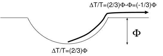
Figure 2.4: The Static Sachs–Wolfe Effect

The static Sachs–Wolfe effect predicts that CMB that resides in a $\Phi$ potential well has an initial adiabatic temperature fluctuation of $\Delta T/T=\frac{2}{3}\Phi$ in the matter era. It further receives an additional fluctuation of $-\Phi$ when climbing up the potential at the decoupling epoch. In total, we observe $\Delta T/T=-\frac{1}{3}\Phi$.

For isocurvature fluctuations, initial temperature fluctuations in a potential well are given by $-\Phi$ in both the radiation era and the matter era; thus, total temperature fluctuations amount to $\Delta T/T=-\Phi-\Phi=-2\Phi$. By definition of the isocurvature fluctuations, $\Phi$ is initially zero, but there exist non-vanishing initial entropy fluctuations. As the universe evolves, the entropy fluctuations create $\Phi$, and hence the temperature fluctuations.

At the decoupling epoch, the universe has already been in the matter era in which $w=0$, so that we observe adiabatic temperature fluctuations of $\Delta T/T=-\frac{1}{3}\Phi=-\frac{1}{5}\zeta$, and the CMB fluctuation spectrum of the Sachs–Wolfe effect, $\Delta_{\rm SW}^{2}(k)$, is

$$\Delta_{\rm SW}^{2}(k)=\frac{1}{9}\Delta_{\Phi}^{2}(k)=\frac{1}{25}\Delta_{\zeta}^{2}(k)=\left[\frac{H^{2}}{10\pi(d\phi/dt)}\right]^{2},$$ (2.49)

where $H$ is the Hubble parameter during inflation. While we have not shown the $k$ dependence of the spectrum here, the spectral index is given by equation (2.44). By projecting the 3-dimension CMB fluctuation spectrum, $\Delta_{\rm SW}^{2}(k)$, on the sky, we obtain the angular power spectrum, $C_{l}$ (BE87),

$$C_{l}^{\rm SW}=4\pi\int_{0}^{\infty}\frac{dk}{k}~{}\Delta_{\rm SW}^{2}(k)j^{2}_{l}\left[k(\tau_{0}-\tau_{\rm dec})\right]=C^{\rm SW}_{2}\frac{\Gamma\left[(9-n)/2\right]\Gamma\left[l+(n-1)/2\right]}{\Gamma\left[(n+3)/2\right]\Gamma\left[l+(5-n)/2\right]},$$ (2.50)

where $\tau_{0}$ and $\tau_{\rm dec}$ denote the present day and the decoupling epoch, respectively, and $n\equiv 1+\left[d\ln\Delta^{2}(k)/d\ln k\right]$ is a spectral index which is conventionally used in the literature. If the spectrum is exactly scale invariant, $n=1$, then we obtain $C_{l}^{\rm SW}=\left[l(l+1)\right]^{-1}6C_{2}^{\rm SW}$.

Equation (2.50) provides a simple yet good fit to the CMB power spectrum measured by COBE DMR. The spectrum comprises two parameters, $C_{2}^{\rm SW}$ and $n$. Ben96 find $n=1.2\pm 0.3$ and $C_{2}^{\rm SW}=7.9^{+2.0}_{-1.4}\times 10^{-11}$. When fixing $n=1$, they find $C_{2}^{\rm SW|n=1}=(9.3\pm 0.8)\times 10^{-11}$. The measured $C_{l}$ is thus consistent with CMB being scale invariant, supporting inflation. Moreover, it implies that $H^{2}/(d\phi/dt)\sim\left(C_{2}^{\rm SW}\right)^{1/2}\sim 10^{-5}$, constraining amplitude of the Hubble parameter during inflation.

On the angular scales smaller than the DMR angular scales, the Sachs–Wolfe approximation breaks down, and the acoustic physics in the photon-baryon fluid system modifies the primordial radiation spectrum (PY70; BE87). To calculate the modification, we have to solve the Boltzmann photon transfer equation together with the Einstein equations. The modification is often described by the radiation transfer function, $g_{{\rm T}l}(k)$, which can be calculated numerically with the Boltzmann code such as CMBFAST (SZ96). Using $g_{{\rm T}l}(k)$, we write the CMB power spectrum, $C_{l}$, as

$$C_{l}=4\pi\int_{0}^{\infty}\frac{dk}{k}~{}\Delta_{\Phi}^{2}(k)g^{2}_{{\rm T}l}(k).$$ (2.51)

Note that for the static Sachs–Wolfe effect, adiabatic fluctuations give $g_{{\rm T}l}(k)=-\frac{1}{3}j_{l}\left[k(\tau_{0}-\tau_{\rm dec})\right]$, while isocurvature fluctuations give $g_{{\rm T}l}(k)=-2j_{l}\left[k(\tau_{0}-\tau_{\rm dec})\right]$. Here, we have used $\Delta_{\Phi}^{2}(k)$ rather than $\Delta_{\rm SW}^{2}(k)$ or $\Delta_{\zeta}^{2}(k)$, following the literature. The literature often uses the $\Phi$ power spectrum, $P_{\Phi}(k)$, to replace $\Delta_{\Phi}^{2}(k)$; the relation is $\Delta_{\Phi}^{2}(k)=(2\pi^{2})^{-1}k^{3}P_{\Phi}(k)$. $\Delta_{\Phi}^{2}(k)$ is called the dimensionless power spectrum.

If $\Phi$ were exactly Gaussian, then $C_{l}$ would specify all the statistical properties of $\Phi$, which are equivalent to those of $\zeta$. Since $\zeta$ is related to a Gaussian variable, $u$, through $\zeta=-(aH/\dot{\phi})u$, in the linear order $\zeta$ also obeys Gaussian statistics; however, the relation between $\zeta$ and $u$ becomes non-linear when we take into account non-linear perturbations. As a result, $\zeta$, and hence $\Phi$, becomes non-Gaussian even if $u$ is exactly Gaussian, yielding non-Gaussian CMB anisotropies. In the next section, we will analyze non-linear perturbations in inflation.

Using the second-order gravitational perturbation theory, PC96 derive the second-order correction to the relation between $\Delta T$ and $\Phi$ (Eq.(2.48)). It gives $\Delta T/T=-\frac{1}{3}\Phi+{\cal O}(1)\Phi^{2}$; thus, even if $\Phi$ is Gaussian, $\Delta T$ becomes weakly non-Gaussian.

2.4 Non-linear Perturbations in Inflation

In the previous section, we have shown that the quantum fluctuations generate the gauge-invariant perturbation, $u=\delta\phi-(\dot{\phi}/aH){\cal R}$, and $u$ obeys Gaussian statistics very well because of the central limit theorem. Another gauge-invariant variable, $\zeta=-(aH/\dot{\phi})u={\cal R}-(aH/\dot{\phi})\delta\phi$, which remains constant in time outside the horizon, also obeys Gaussian statistics in the linear order, as it is related to a Gaussian variable, $u$, linearly.

In the non-linear order, however, the situation may change. In the relation between $\zeta$ and $u$, the factor in front of $u$, $aH/\dot{\phi}$, is also a function of $\phi$, and it may produce additional fluctuations like $[\partial(aH/\dot{\phi})/\partial\phi]\delta\phi$. Suppose that ${\cal R}$ in the comoving gauge ($\delta\phi_{\rm com}\equiv 0$), ${\cal R}_{\rm com}$, is an arbitrary function of a scalar field: ${\cal R}_{\rm com}=f(\phi)$. Note that ${\cal R}_{\rm com}$ is equivalent to $\zeta$. By perturbing $\phi$ as $\phi=\phi_{0}+\delta\phi_{\rm flat}$, where $\delta\phi_{\rm flat}$ is a scalar-field fluctuation in the spatially flat gauge (${\cal R}_{\rm flat}\equiv 0$), we have

$${\cal R}_{\rm com} = f(\phi_{0}+\delta\phi_{\rm flat})$$ (2.52)

$$= f(\phi_{0})+\left(\frac{\partial f}{\partial\phi}\right)\delta\phi_{\rm flat}+\frac{1}{2}\left(\frac{\partial^{2}f}{\partial\phi^{2}}\right)\delta\phi^{2}_{\rm flat}+{\cal O}\left(\delta\phi_{\rm flat}^{3}\right).$$

By comparing this equation with the linear-perturbation result (Eq.(2.39)), ${\cal R}_{\rm com}=-(aH/\dot{\phi})\delta\phi_{\rm flat}$, we find $f(\phi_{0})=0$, $\partial f/\partial\phi=-(aH/\dot{\phi})$, and

$${\cal R}_{\rm com}=-\frac{aH}{\dot{\phi}}\delta\phi_{\rm flat}-\frac{1}{2}\frac{\partial}{\partial\phi}\left(\frac{aH}{\dot{\phi}}\right)\delta\phi^{2}_{\rm flat}+{\cal O}\left(\delta\phi_{\rm flat}^{3}\right);$$ (2.53)

thus, even if $\delta\phi_{\rm flat}$ is exactly Gaussian, ${\cal R}_{\rm com}$, and hence $\zeta$, becomes weakly non-Gaussian because of $\delta\phi_{\rm flat}^{2}$ or the higher-order terms. While the treatment here may look rather crude, we will show in this section that the solution (Eq.(2.53)) actually satisfies a more proper treatment of non-linear perturbations in inflation.

In the linear regime, we have the gauge-invariant perturbation variable that characterizes the curvature perturbations as well as the scalar-field fluctuations, and the single equation that describes the perturbation evolution on all scales. In the non-linear regime, however, we cannot make such great simplification. Since the Einstein equations are highly non-linear, fully analyzing non-linear problems is technically very difficult. Hence, we need a certain approximation.

2.4.1 Gradient expansion of Einstein equations

In inflation, there is an useful scheme of approximation, the so-called anti-Newtonian approximation (Tom75; Tom82; TD92), or later called the long-wavelength approximation (KH98; ST98) or the gradient expansion method (SB90; SS92; NT96; NT98).

The approximation neglects higher-order spatial derivatives in the Einstein equations as well as in the equations of motion for matter fields, and is equivalent to taking a long-wavelength limit of the system. The equation system is further simplified if we set the shift vector zero in the metric. Once neglecting higher-order spatial derivatives and the shift vector, one finds that the shear decays away very rapidly.

We use the metric of the form

$$ds^{2}=-N^{2}d\tau^{2}+{}^{(3)}g_{ij}dx^{i}dx^{j},$$ (2.54)

where $N$ is the Lapse function, and ${}^{(3)}g_{ij}$ describes the 3-metric. We have set the shift vector zero; it corresponds to $B\equiv 0$ in the linearized metric (2.29). We perturb $N$ and ${}^{(3)}g_{ij}$ non-linearly. While the full treatment of non-linear evolution of the system is highly complicated, by neglecting higher-order spatial derivatives, we reduce the Einstein equations to rather simplified forms (SB90):

$$H^{2}-\frac{1}{3}\sigma^{ij}\sigma_{ij} = \frac{8\pi G}{3}\left[\frac{1}{2N^{2}}\dot{\phi}^{2}+V(\phi)\right],$$ (2.55)

$$H_{,i}-\frac{1}{2}\sigma^{k}_{i,k} = -4\pi G\frac{\dot{\phi}}{N}\phi_{,i},$$ (2.56)

$$\frac{2}{N}\dot{H}+3H^{2}+\sigma^{ij}\sigma_{ij} = -8\pi G\left[\frac{1}{2N^{2}}\dot{\phi}^{2}-V(\phi)\right],$$ (2.57)

$$\frac{1}{N}\dot{\sigma}^{i}_{j}+3H\sigma^{i}_{j} = 0.$$ (2.58)

$H$ is the inhomogeneous Hubble parameter which defines the isotropic expansion rate of the $\tau={\rm constant}$ hypersurfaces,

$$H\equiv\frac{1}{6N}{}^{(3)}g^{ij}{}^{(3)}\dot{g}_{ij},$$ (2.59)

or ${}^{(3)}\dot{g}_{ij}=2NH{}^{(3)}g_{ij}$. By introducing the inhomogeneous scale factor, $a({\mathbf{x}},\tau)$, given by $H=\dot{a}/(Na)$, we can write the 3-metric as ${}^{(3)}g_{ij}=a^{2}({\mathbf{x}},\tau)\gamma_{ij}({\mathbf{x}})$, where $\gamma_{ij}({\mathbf{x}})$ is a function of the spatial coordinate only. This form of ${}^{(3)}g_{ij}$ satisfies equation (2.59). We have obtained the simplified form for the 3-metric because of setting the shift vector zero.

$\sigma^{i}_{j}$ is the shear which quantifies the anisotropic expansion rate,

$$\sigma^{i}_{j}\equiv\frac{1}{2N}{}^{(3)}\dot{g}_{ij}-H{}^{(3)}g_{ij}.$$ (2.60)

It follows from the traceless-part equation (2.58) and $NH=\dot{a}/a$ that the shear decays rapidly as the universe expands: $\sigma^{i}_{j}\propto a^{-3}$; thus, we neglect the shear terms in the Einstein equations henceforth.

By neglecting the shear term in the trace-part equation (2.57), and substituting the Friedmann equation (2.55) for $H^{2}$, we obtain $\dot{H}=-4\pi GN^{-1}{\dot{\phi}^{2}}$. Comparing this equation with the momentum constraint equation (2.56) without the shear term, ${H}_{,i}=-4\pi GN^{-1}\dot{\phi}{\phi}_{,i}$, we find $H({\mathbf{x}},\tau)=H\left(\phi({\mathbf{x}},\tau)\right)$, and the scalar-field momentum

$$\frac{\dot{\phi}}{N}=-\frac{1}{4\pi G}\left(\frac{\partial H}{\partial\phi}\right).$$ (2.61)

Substituting this for the kinetic term in the Friedmann equation (2.55), and neglecting the shear term, we finally obtain a closed evolution equation for $H(\phi)$,

$$H^{2}(\phi)=\frac{1}{12\pi G}\left(\frac{\partial H}{\partial\phi}\right)^{2}+\frac{8\pi G}{3}V(\phi).$$ (2.62)

From this equation, $H(\phi)$ may be solved as $H(\phi,I)$, where $I$ is an integration constant which parameterizes the initial condition. This equation fully describes the evolution of the system including non-linear perturbations. Note that $H(\phi)$ depends upon the spatial coordinate through $\phi=\phi({\mathbf{x}},\tau)$.

A perturbation to $H$ is given by $\delta H=\left(\partial H/\partial\phi\right)_{I}\delta\phi+\left(\partial H/\partial I\right)_{\phi}\delta I$. For the latter term, by differentiating equation (2.62) with respect to $I$ for a fixed $\phi$, we find $\left(\partial H/\partial I\right)_{\phi}\propto a^{-3}$; thus, it decays very rapidly during inflation, giving $\delta H=\left(\partial H/\partial\phi\right)_{I}\delta\phi$. Hence, the comoving gauge, $\delta\phi\equiv 0$, coincides with the constant Hubble parameter gauge, $\delta H\equiv 0$. ST98 also observe this property from a different point of view, and find that this property holds for multiple scalar-field system as well.

2.4.2 Generation of non-linear curvature perturbations

Our goal in this subsection is to find a non-linear relation between ${\cal R}_{\rm com}$ and $\delta\phi_{\rm flat}$, following SB90. In the absence of the shear, ${\cal R}$ obeys $\dot{\cal R}=\delta\left(NH\right)=\delta\left(\partial\ln a/\partial\tau\right)$, and hence ${\cal R}$ is equivalent to fluctuations in the inhomogeneous scale factor, $\delta\ln a$.

We calculate ${\cal R}_{\rm com}$ by perturbing $\ln a$ non-linearly in the comoving gauge. Since $\phi$ is homogeneous in the comoving gauge, we choose $\phi$ as a time coordinate: $\tau\equiv\phi$. We find the Lapse function

$$N=-\frac{4\pi G}{\partial H/\partial\phi}$$ (2.63)

for this time coordinate from equation (2.61) with setting $\dot{\phi}\equiv 1$.

To calculate the scalar-field fluctuations in the spatially flat gauge, $\delta\phi_{\rm flat}$, we need to generate quantum fluctuations first; however, since we are solving the equation system on super-horizon scales only, we cannot calculate quantum fluctuations of $\delta\phi$ within the current framework. Instead, we assume that $\delta\phi$ on super-horizon scales is provided by the small-scale quantum fluctuations that are stretched out of the horizon by inflationary expansion. We use the linear perturbation theory to calculate the fluctuation amplitude at the horizon crossing, and provide $\delta\phi$ as initially linear, Gaussian fluctuations. We then calculate $\delta\phi_{\rm flat}$ on the $\ln a={\rm constant}$ hypersurfaces. While this treatment may sacrifice a virtue of the current framework which does not assume linearity of perturbations, non-linearity of the scalar-field fluctuations may also be incorporated into the analysis with the so-called stochastic inflation approach (Sta86; SB91). Using this, Gan94 show that the non-linearity makes $\delta\phi_{\rm flat}$ weakly non-Gaussian.

After all, our goal is to relate $\delta\phi(\ln a)$ to $\delta\ln a(\phi)$. In other words, we transform the perturbations on the $\ln a={\rm constant}$ hypersurfaces to the ones on the $\phi={\rm constant}$ hypersurfaces. We do this as follows (SB90), and figure (2.5) shows the following process schematically.

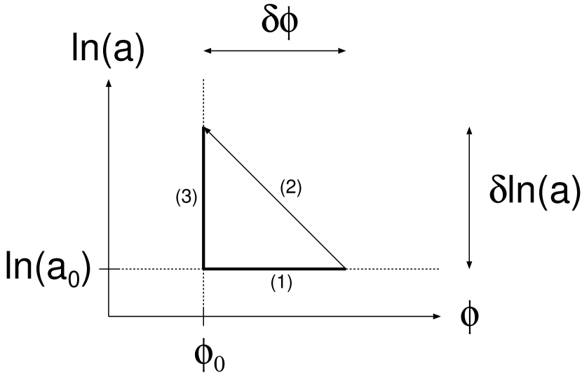
Figure 2.5: Hypersurface Transformation

Hypersurface transformation of the scalar-field fluctuations in the spatially flat gauge, $\delta\phi_{\rm flat}=\delta\phi(\ln a_{0})$, into the spatial curvature perturbations in the comoving gauge, ${\cal R}_{\rm com}=\delta\ln a(\phi_{0})$. (1) To represent $\delta\phi(\ln a_{0})$, draw a short line from $(\phi_{0},\ln a_{0})$ to $(\phi_{0}+\delta\phi,\ln a_{0})$ in parallel to the $\phi$ axis. (2) By evolving $\ln a$, evolve this line until it coincides with the $\phi=\phi_{0}$ line. (3) Measure the line length, $\delta\ln a(\phi_{0})$.

First, imagine $\phi-\ln a$ plane on which we transform the perturbations. We then mark a point on the plane with $(\phi_{0},\ln a_{0})$, and draw a short line from this point to $(\phi_{0}+\delta\phi,\ln a_{0})$ in parallel to the $\phi$ axis. This line represents $\delta\phi({\mathbf{x}},\ln a_{0})\equiv\phi({\mathbf{x}},\ln a_{0})-\phi_{0}$, i.e., $\phi$ perturbations on a $\ln a=\ln a_{0}$ hypersurface. Next, using evolution equation of $\ln a$, we evolve the line until it coincides with the $\phi=\phi_{0}$ line, namely

$$\ln a_{0}=\ln\left[a({\mathbf{x}},\phi_{0}+\delta\phi)\right]\longrightarrow\ln\left[a({\mathbf{x}},\phi_{0})\right].$$ (2.64)

The evolution equation of $\ln a$ is $d\ln a/d\tau=NH$. By integrating this equation, we obtain

$$\ln\left[a({\mathbf{x}},\phi_{0})\right]-\ln a_{0}=\int_{\phi_{0}+\delta\phi({\mathbf{x}},\ln a_{0})}^{\phi_{0}}d\phi~{}\frac{N(\phi)H(\phi)}{\dot{\phi}},$$ (2.65)

where the Lapse function, $N$, is given by equation (2.63) for $\phi$ being the time coordinate. Finally, we measure the line length, $\delta\ln\left[a({\mathbf{x}},\phi_{0})\right]\equiv\ln\left[a({\mathbf{x}},\phi_{0})\right]-\ln a_{0}$, to obtain ${\cal R}_{\rm com}$.

By noting $\delta\phi_{\rm flat}=\delta\phi({\mathbf{x}},\ln a_{0})$, we find a non-linear relationship between ${\cal R}_{\rm com}$ and $\delta\phi_{\rm flat}$,

$${\cal R}_{\rm com}=-\int_{\phi_{0}}^{\phi_{0}+\delta\phi_{\rm flat}}d\phi~{}\frac{N(\phi)H(\phi)}{\dot{\phi}}=4\pi G\int_{\phi_{0}}^{\phi_{0}+\delta\phi_{\rm flat}}d\phi\left[\frac{\partial\ln H}{\partial\phi}\right]^{-1}.$$ (2.66)

This non-linear relation should be compared with the crude estimate from the linear analysis, equation (2.53). By expanding the non-linear relation into Taylor series with respect to $\delta\phi_{\rm flat}$, we find that the crude estimate agrees with the non-linear result on the term-by-term basis. Note that $a$ in equation (2.53) should be replaced by $N$, as it has used the conformal time as the time coordinate, i.e., $N=a$.

2.4.3 Generation of weakly non-Gaussian adiabatic fluctuations

We have shown that non-linearity in inflation creates weakly non-Gaussian curvature perturbations outside the horizon from Gaussian quantum fluctuations inside the horizon. By expanding the non-linear relation between ${\cal R}_{\rm com}$ and $\delta\phi_{\rm flat}$ up to the second order, we obtain a non-linear curvature perturbation, ${\cal R}_{\rm com}={\cal R}_{\rm com}^{\rm L}+{\cal R}_{\rm com}^{\rm NL}$, where

$${\cal R}_{\rm com}^{\rm L} \equiv {4\pi G}\left(\frac{\partial\ln H}{\partial\phi}\right)^{-1}\delta\phi_{\rm flat},$$ (2.67)

$${\cal R}_{\rm com}^{\rm NL} \equiv -\frac{1}{8\pi G}\left(\frac{\partial^{2}\ln H}{\partial\phi^{2}}\right)\left({\cal R}_{\rm com}^{\rm L}\right)^{2}.$$ (2.68)

Using equation (2.46), we obtain a non-linear Newtonian potential, $\Phi=\Phi_{\rm L}+\Phi_{\rm NL}$, where $\Phi_{\rm L}=\frac{2}{3}{\cal R}_{\rm com}^{\rm L}$ and $\Phi_{\rm NL}=\frac{2}{3}{\cal R}_{\rm com}^{\rm NL}$ in the radiation era, and $\Phi_{\rm L}=\frac{3}{5}{\cal R}_{\rm com}^{\rm L}$ and $\Phi_{\rm NL}=\frac{3}{5}{\cal R}_{\rm com}^{\rm NL}$ in the matter era. Note that these formulae should be modified when we include non-linear effects of the stochastic inflation approach (Gan94), which add extra terms to the formulae.

In the following chapters, we will focus on measuring $\Phi_{\rm NL}$ using non-Gaussian CMB temperature fluctuations. We parameterize the amplitude of $\Phi_{\rm NL}$ with a non-linear coupling parameter, $f_{\rm NL}$, as

$$\Phi_{\rm NL}\left({\mathbf{x}}\right)=f_{\rm NL}\left[\Phi_{\rm L}^{2}\left({\mathbf{x}}\right)-\left<\Phi_{\rm L}^{2}\left({\mathbf{x}}\right)\right>\right].$$ (2.69)

How big is $f_{\rm NL}$? If a scalar field rolls down on a potential, $V(\phi)$, slowly, then $\partial\ln H/\partial\phi\approx\frac{1}{2}\partial\ln V/\partial\phi$. We thus obtain

$$f_{\rm NL}=-\frac{5}{24\pi G}\left(\frac{\partial^{2}\ln H}{\partial\phi^{2}}\right)\approx-\frac{5}{48\pi G}\left(\frac{\partial^{2}\ln V}{\partial\phi^{2}}\right).$$ (2.70)

As an example, consider a power-law potential, $V(\phi)\propto\phi^{n}$. We find

$$f_{\rm NL}=\frac{5n}{48\pi}\frac{m_{\rm pl}^{2}}{\phi^{2}}\sim 10^{-2}.$$ (2.71)

On the other hand, we will show in chapter 4 that $\left|f_{\rm NL}\right|$ should be larger than of order unity to produce detectable non-Gaussian signals in CMB. Even for the fastest motion of $\phi$ allowed in slowly-rolling single-field inflation, we find $\left|f_{\rm NL}\right|<5/2$. Therefore, it is quite hard for this class of inflation models to produce detectable CMB non-Gaussianity. In other words, any detection of cosmological non-Gaussian signals in CMB constrains slow-roll inflation models very strongly, or may favor multiple scalar-field models or isocurvature fluctuations.

Chapter 3 Angular $n$-point Harmonic Spectrum on the Sky

The angular $n$-point correlation function,

$$\left<f(\hat{\mathbf{n}}_{1})f(\hat{\mathbf{n}}_{2})\dots f(\hat{\mathbf{n}}_{n})\right>,$$ (3.1)

is a simple statistic characterizing a clustering pattern of fluctuations on the sky, $f(\hat{\mathbf{n}})$. Here, the bracket denotes the ensemble average, and figure 3.1 sketches the meaning. If the fluctuation is Gaussian, then the two-point correlation function specifies all the statistical properties of $f(\hat{\mathbf{n}})$, for the two-point correlation function is the only parameter in Gaussian distribution. If it is not Gaussian, then we need higher-order correlation functions to determine the statistical properties.

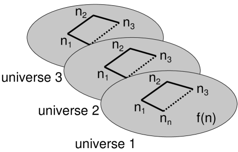
Figure 3.1: Ensemble Average of Angular Correlation Function

A schematic view of the ensemble average of the $n$-point angular correlation function, $f(\hat{\mathbf{n}}_{1})f(\hat{\mathbf{n}}_{2})f(\hat{\mathbf{n}}_{3})\dots f(\hat{\mathbf{n}}_{n})$. We measure it on each universe, and then average it over many universes.

Yet simple, one disadvantage of the angular correlation function is that data points of the correlation function at different angular scales are generally not independent of each other, but correlated: two-point correlation at 1 degree is correlated with that at 2 degrees, and so on. This property makes a detailed statistical analysis and interpretation of the data complicated.

Hence, one finds it more convenient to expand $f(\hat{\mathbf{n}})$ into spherical harmonics, the orthonormal basis on the sphere, as

$$f(\hat{\mathbf{n}})=\sum_{l=0}^{\infty}\sum_{m=-l}^{l}a_{lm}Y_{lm}(\hat{\mathbf{n}}),$$ (3.2)

and then to consider the angular $n$-point harmonic spectrum, $\left<a_{l_{1}m_{1}}a_{l_{2}m_{2}}\dots a_{l_{n}m_{n}}\right>$. While $a_{lm}$ for $m\neq 0$ is complex, reality of $f(\hat{\mathbf{n}})$ gives $a_{l-m}=a_{lm}^{*}(-1)^{m}$, and thus the number of independent modes is not $4l+1$, but $2l+1$.

Especially, the angular two-, three-, and four-point harmonic spectra are called the angular power spectrum, bispectrum, and trispectrum, respectively. For a Gaussian field, the angular spectra at different angular scales, or at different $l$’s, are uncorrelated. Even for a non-Gaussian field, they are reasonably uncorrelated as long as the non-Gaussianity is weak. Moreover, since the spherical harmonic is orthogonal for different $l$’s, it highlights characteristic structures on the sky at a given $l$. In other words, even if the angular correlation function is featureless, the angular spectrum may have a distinct structure, for inflation predicts a prominent peak in the angular power spectrum, not in the angular correlation function. In this chapter, we study statistical properties of the angular $n$-point harmonic spectra.

3.1 Statistical Isotropy of the Universe

In reality, we cannot measure the ensemble average of the angular harmonic spectrum, but one realization such as $a_{l_{1}m_{1}}a_{l_{2}m_{2}}\dots a_{l_{n}m_{n}}$, which is so noisy that we want to average it somehow to reduce the noise.

We assume statistical isotropy of the universe from which it follows that our sky is isotropic and has no preferred direction. Isotropy of CMB justifies the assumption. The assumption readily implies that one can average the spectrum over $m_{i}$ with an appropriate weight, as $m_{i}$ represent an azimuthal orientation on the sky. The average over $m_{i}$ enables us to reduce statistical error of the measured harmonic spectra.

How can we find the weight? One finds it as a solution to statistical isotropy, or rotational invariance of the angular correlation function on the sky,

$$\left<Df(\hat{\mathbf{n}}_{1})Df(\hat{\mathbf{n}}_{2})\dots Df(\hat{\mathbf{n}}_{n})\right>=\left<f(\hat{\mathbf{n}}_{1})f(\hat{\mathbf{n}}_{2})\dots f(\hat{\mathbf{n}}_{n})\right>,$$ (3.3)

where $D=D(\alpha,\beta,\gamma)$ is a rotation matrix for the Euler angles $\alpha$, $\beta$, and $\gamma$. Figure 3.2 sketches the meaning of statistical isotropy. Substituting equation (3.2) for $f(\hat{\mathbf{n}})$ in equation (3.3), we then need rotation of the spherical harmonic, $DY_{lm}(\hat{\mathbf{n}})$. It is formally represented by the rotation matrix element, $D_{m^{\prime}m}^{(l)}(\alpha,\beta,\gamma)$, as (RBMW59)

$$DY_{lm}(\hat{\mathbf{n}})=\sum_{m^{\prime}=-l}^{l}D_{m^{\prime}m}^{(l)}Y_{lm^{\prime}}(\hat{\mathbf{n}}).$$ (3.4)

The matrix element, $D_{m^{\prime}m}^{(l)}=\left<l,m^{\prime}\left|D\right|l,m\right>$, describes finite rotation of an initial state whose orbital angular momentum is represented by $l$ and $m$ into a final state represented by $l$ and $m^{\prime}$. Finally, we obtain the statistical isotropy condition on the angular $n$-point harmonic spectrum:

$$\left<a_{l_{1}m_{1}}a_{l_{2}m_{2}}\dots a_{l_{n}m_{n}}\right>=\sum_{{\rm all}~{}m^{\prime}}\left<a_{l_{1}m^{\prime}_{1}}a_{l_{2}m^{\prime}_{2}}\dots a_{l_{n}m^{\prime}_{n}}\right>D_{m_{1}^{\prime}m_{1}}^{(l_{1})}D_{m_{2}^{\prime}m_{2}}^{(l_{2})}\dots D_{m^{\prime}_{n}m_{n}}^{(l_{n})}.$$ (3.5)

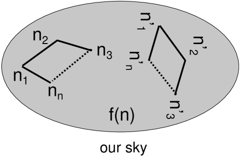
Figure 3.2: Statistical Isotropy of Angular Correlation Function

A schematic view of statistical isotropy of the angular correlation function. As long as its configuration is preserved, we can average $f(\hat{\mathbf{n}}_{1})\dots f(\hat{\mathbf{n}}_{n})$ over all possible orientations and positions on the sky.

Using this equation, Hu01 has systematically evaluated appropriate weights for averaging the angular power spectrum ($n=2$), bispectrum ($n=3$), and trispectrum ($n=4$), over azimuthal angles. Some of those may be found more intuitively; however, this method allows us to find the weight for any higher-order harmonic spectrum. In the following sections, we derive rotationally invariant, azimuthally averaged harmonic spectra for $n=2$, 3, and 4, and study their statistical properties.

3.2 Angular Power Spectrum

The angular power spectrum measures how much fluctuations exist on a given angular scale. For example, the variance of $a_{lm}$ for $l\geq 1$, $\left<a_{lm}a_{lm}^{*}\right>$, measures the amplitude of fluctuations at a given $l$.

Generally speaking, the covariance matrix of $a_{lm}$, $\left<a_{l_{1}m_{1}}a_{l_{2}m_{2}}^{*}\right>$, is not necessarily diagonal. It is, however, actually diagonal once we assume full sky coverage and rotational invariance of the angular two-point correlation function, as we will show in this section. The variance of $a_{lm}$ thus describes the two-point correlation completely.

Rotational invariance (Eq.(3.5)) requires

$$\left<a_{l_{1}m_{1}}a^{*}_{l_{2}m_{2}}\right>=\sum_{m_{1}^{\prime}m_{2}^{\prime}}\left<a_{l_{1}m^{\prime}_{1}}a^{*}_{l_{2}m^{\prime}_{2}}\right>D_{m_{1}^{\prime}m_{1}}^{(l_{1})}D_{m^{\prime}_{2}m_{2}}^{(l_{2})*}$$ (3.6)

to be satisfied, where we have used the complex conjugate for simplifying calculations. From this equation, we seek for a rotationally invariant representation of the angular power spectrum. Suppose that the covariance matrix of $a_{lm}$ is diagonal, i.e., $\left<a_{l_{1}m_{1}}a^{*}_{l_{2}m_{2}}\right>=\left<C_{l_{1}}\right>\delta_{l_{1}l_{2}}\delta_{m_{1}m_{2}}$. Equation (3.6) then reduces to

$$\left<a_{l_{1}m_{1}}a^{*}_{l_{2}m_{2}}\right>=\left<C_{l_{1}}\right>\delta_{l_{1}l_{2}}\sum_{m_{1}^{\prime}}D_{m_{1}^{\prime}m_{1}}^{(l_{1})}D_{m^{\prime}_{1}m_{2}}^{(l_{1})*}=\left<C_{l_{1}}\right>\delta_{l_{1}l_{2}}\delta_{m_{1}m_{2}}.$$

Thus, we have proven $\left<C_{l}\right>$ rotationally invariant. Rotational invariance implies that the covariance matrix is diagonal.

3.2.1 Estimator

Observationally, the unbiased estimator of $\left<C_{l}\right>$ should be

$$C_{l} = \frac{1}{2l+1}\sum_{m=-l}^{l}a_{lm}a_{lm}^{*}=\frac{1}{2l+1}\left(a_{l0}^{2}+2\sum_{m=1}^{l}a_{lm}a_{lm}^{*}\right)$$ (3.7)

$$= \frac{1}{2l+1}\left\{a_{l0}^{2}+2\sum_{m=1}^{l}\left[\left(\Re{a_{lm}}\right)^{2}+\left(\Im{a_{lm}}\right)^{2}\right]\right\}.$$

The second equality follows from $a_{l-m}=a_{lm}^{*}(-1)^{m}$, i.e., $a_{l-m}a_{l-m}^{*}=a_{lm}a_{lm}^{*}$, and hence we average $2l+1$ independent samples for a given $l$. It suggests that fractional statistical error of $C_{l}$ is reduced by $\sqrt{1/(2l+1)}$. This property is the main motivation of our considering the azimuthally averaged harmonic spectrum.

We find it useful to define an azimuthally averaged harmonic transform, $e_{l}(\hat{\mathbf{n}})$, as

$$e_{l}(\hat{\mathbf{n}})\equiv\sqrt{\frac{4\pi}{2l+1}}\sum_{m=-l}^{l}a_{lm}Y_{lm}(\hat{\mathbf{n}}),$$ (3.8)

which is interpreted as a square-root of $C_{l}$ at a given position of the sky,

$$\int\frac{d^{2}\hat{\mathbf{n}}}{4\pi}~{}e^{2}_{l}(\hat{\mathbf{n}})=C_{l}.$$ (3.9)

$e_{l}(\hat{\mathbf{n}})$ is particularly useful for measuring the angular bispectrum (SG99; Kom01b) (chapter 5), trispectrum (chapter 6), and probably any higher-order harmonic spectra, because of being computationally very fast to calculate. This is very important, as the new satellite experiments, MAP and Planck, have more than millions of pixels, for which we will crucially need a fast algorithm of measuring these higher-order harmonic spectra.

3.2.2 Covariance matrix

We derive the covariance matrix of $C_{l}$, $\left<C_{l}C_{l^{\prime}}\right>-\left<C_{l}\right>\left<C_{l^{\prime}}\right>$, with the four-point function, the trispectrum. Starting with

$$\left<C_{l}C_{l^{\prime}}\right>=\frac{1}{(2l+1)(2l^{\prime}+1)}\sum_{mm^{\prime}}\left<a_{lm}a_{lm}^{*}a_{l^{\prime}m^{\prime}}a_{l^{\prime}m^{\prime}}^{*}\right>,$$ (3.10)

we obtain the power spectrum covariance matrix

$$\left<C_{l}C_{l^{\prime}}\right>-\left<C_{l}\right>\left<C_{l^{\prime}}\right> = \frac{2\left<C_{l}\right>^{2}}{2l+1}\delta_{ll^{\prime}}+\frac{1}{(2l+1)(2l^{\prime}+1)}\sum_{mm^{\prime}}\left<a_{lm}a_{lm}^{*}a_{l^{\prime}m^{\prime}}a_{l^{\prime}m^{\prime}}^{*}\right>_{\rm c}$$ (3.11)

$$= \frac{2\left<C_{l}\right>^{2}}{2l+1}\delta_{ll^{\prime}}+\frac{(-1)^{l+l^{\prime}}}{\sqrt{(2l+1)(2l^{\prime}+1)}}\left<T^{ll}_{l^{\prime}l^{\prime}}(0)\right>_{\rm c},$$

where $\left<a_{lm}a_{lm}^{*}a_{l^{\prime}m^{\prime}}a_{l^{\prime}m^{\prime}}^{*}\right>_{\rm c}$ is the connected four-point harmonic spectrum, the connected trispectrum, which is exactly zero for a Gaussian field. It follows from this equation that the covariance matrix of $C_{l}$ is exactly diagonal only when $a_{lm}$ is Gaussian. $\left<T^{l_{1}l_{2}}_{l_{3}l_{4}}(L)\right>_{\rm c}$ is the ensemble average of the angular averaged connected trispectrum, which we will define in § 3.4 (Eq.(3.46)).

Unfortunately, we cannot measure the connected $T^{ll}_{l^{\prime}l^{\prime}}(0)$ directly from the angular trispectrum (see § 3.4). We will thus never be sure if the power spectrum covariance is precisely diagonal, as long as we use the angular trispectrum. We need the other statistics that can pick up information of the connected $T^{ll}_{l^{\prime}l^{\prime}}(0)$, even though they are indirect. Otherwise, we need a model for the connected trispectrum, and use the model to constrain the connected $T^{ll}_{l^{\prime}l^{\prime}}(0)$ from the other trispectrum configurations. We will discuss this point in chapter 6.

There is no reason to assume the connected $T^{ll}_{l^{\prime}l^{\prime}}(0)$ small. It is produced on large angular scales, if topology of the universe is closed hyperbolic (Ino01b). In appendix LABEL:app:CH, we derive an analytic prediction for the connected trispectrum produced in a closed hyperbolic universe. On small angular scales, several authors have shown that the weak gravitational lensing effect produces the connected trispectrum or four-point correlation function (Ber97; ZS99; Zal00); Hu01 finds that the induced off-diagonal terms are negligible compared with the diagonal terms out to $l\sim 2000$.

If the connected trispectrum is negligible, then we obtain

$$\left<C_{l}C_{l^{\prime}}\right>-\left<C_{l}\right>\left<C_{l^{\prime}}\right>\approx\frac{2\left<C_{l}\right>^{2}}{2l+1}\delta_{ll^{\prime}}.$$ (3.12)

The fractional error of $C_{l}$ is thus proportional to $\sqrt{1/(2l+1)}$, as expected from our having $2l+1$ independent samples to average for a given $l$. The exact form follows from $C_{l}$ being $\chi^{2}$ distribution with $2l+1$ degrees of freedom when $a_{lm}$ is Gaussian. If $a_{lm}$ is Gaussian, then its probability density distribution is

$$P\left(a_{lm}\right)=\frac{\exp\left[-{a_{lm}^{2}}/(2\left<C_{l}\right>)\right]}{\sqrt{2\pi\left<C_{l}\right>}}.$$ (3.13)

We use this distribution to generate Gaussian random realizations of $a_{lm}$ for a given $\left<C_{l}\right>$. First, we calculate $\left<C_{l}\right>$ with the CMBFAST code (SZ96) for a set of cosmological parameters. We then generate a realization of $a_{lm}$, $a_{lm}=\epsilon\left<C_{l}\right>^{1/2}$, where $\epsilon$ is a Gaussian random variable with the unit variance.

3.3 Angular Bispectrum

The angular bispectrum consists of three harmonic transforms, $a_{l_{1}m_{1}}a_{l_{2}m_{2}}a_{l_{3}m_{3}}$. For Gaussian $a_{lm}$, the expectation value is exactly zero. By imposing statistical isotropy upon the angular three-point correlation function, one finds that the angular averaged bispectrum, $B_{l_{1}l_{2}l_{3}}$, given by

$$\left<a_{l_{1}m_{1}}a_{l_{2}m_{2}}a_{l_{3}m_{3}}\right>=\left<B_{l_{1}l_{2}l_{3}}\right>\left(\begin{array}[]{ccc}l_{1}&l_{2}&l_{3}\\ m_{1}&m_{2}&m_{3}\end{array}\right)$$ (3.14)

satisfies rotational invariance (Eq.(3.5)). Here, the matrix denotes the Wigner-$3j$ symbol (see appendix LABEL:app:wigner). Since $l_{1}$, $l_{2}$, and $l_{3}$ form a triangle, $B_{l_{1}l_{2}l_{3}}$ satisfies the triangle condition, $\left|l_{i}-l_{j}\right|\leq l_{k}\leq l_{i}+l_{j}$ for all permutations of indices. Parity invariance of the angular correlation function demands $l_{1}+l_{2}+l_{3}={\rm even}$. Figure 3.3 sketches a configuration of the angular bispectrum.

Figure 3.3: Angular Bispectrum Configuration

The Wigner-$3j$ symbol, which describes coupling of two angular momenta, represents the azimuthal angle dependence of the angular bispectrum, for the bispectrum forms a triangle. Suppose that two “states” with $(l_{1},m_{1})$ and $(l_{2},m_{2})$ angular momenta form a coupled state with $(l_{3},m_{3})$. They form a triangle whose orientation is represented by $m_{1}$, $m_{2}$, and $m_{3}$, with satisfying $m_{1}+m_{2}+m_{3}=0$. As we rotate the system, the Wigner-$3j$ symbol transforms $m$’s, yet preserving the configuration of the triangle. Similarly, rotational invariance of the angular bispectrum demands that the same triangle configuration give the same amplitude of the bispectrum regardless of its orientation, and thus the Wigner-$3j$ symbol describes the azimuthal angle dependence.

The proof of $\left<B_{l_{1}l_{2}l_{3}}\right>$ to be rotationally invariant is as follows. Substituting equation (3.14) for the statistical isotropy condition (Eq.(3.5)) for $n=3$, we obtain

$$\left<a_{l_{1}m_{1}}a_{l_{2}m_{2}}a_{l_{3}m_{3}}\right>$$ (3.22)

$$= \sum_{{\rm all}~{}m^{\prime}}\left<a_{l_{1}m_{1}^{\prime}}a_{l_{2}m_{2}^{\prime}}a_{l_{3}m_{3}^{\prime}}\right>D_{m_{1}^{\prime}m_{1}}^{(l_{1})}D_{m_{2}^{\prime}m_{2}}^{(l_{2})}D_{m_{3}^{\prime}m_{3}}^{(l_{3})}$$

$$= \left<B_{l_{1}l_{2}l_{3}}\right>\sum_{{\rm all}~{}m^{\prime}}\left(\begin{array}[]{ccc}l_{1}&l_{2}&l_{3}\\ m_{1}^{\prime}&m_{2}^{\prime}&m_{3}^{\prime}\end{array}\right)$$

$$\times\sum_{LMM^{\prime}}\left(\begin{array}[]{ccc}l_{1}&l_{2}&L\\ m_{1}^{\prime}&m_{2}^{\prime}&M^{\prime}\end{array}\right)\left(\begin{array}[]{ccc}l_{1}&l_{2}&L\\ m_{1}&m_{2}&M\end{array}\right)(2L+1)D_{M^{\prime}M}^{(L)*}D_{m_{3}^{\prime}m_{3}}^{(l_{3})}$$

$$= \left<B_{l_{1}l_{2}l_{3}}\right>\sum_{m_{3}^{\prime}}\sum_{LMM^{\prime}}\delta_{l_{3}L}\delta_{m_{3}^{\prime}M^{\prime}}\left(\begin{array}[]{ccc}l_{1}&l_{2}&L\\ m_{1}&m_{2}&M\end{array}\right)D_{M^{\prime}M}^{(L)*}D_{m_{3}^{\prime}m_{3}}^{(l_{3})}$$ (3.25)

$$= \left<B_{l_{1}l_{2}l_{3}}\right>\left(\begin{array}[]{ccc}l_{1}&l_{2}&l_{3}\\ m_{1}&m_{2}&m_{3}\end{array}\right).$$ (3.28)

In the second equality, we have reduced $D_{m_{1}^{\prime}m_{1}}^{(l_{1})}D_{m_{2}^{\prime}m_{2}}^{(l_{2})}$ to $D_{M^{\prime}M}^{(L)*}$, using equation (LABEL:eq:rotreduce). In the third equality, we have used the identity (RBMW59),

$$\sum_{m^{\prime}_{1}m^{\prime}_{2}}\left(\begin{array}[]{ccc}l_{1}&l_{2}&l_{3}\\ m^{\prime}_{1}&m^{\prime}_{2}&m^{\prime}_{3}\end{array}\right)\left(\begin{array}[]{ccc}l_{1}&l_{2}&L\\ m^{\prime}_{1}&m^{\prime}_{2}&M^{\prime}\end{array}\right)=\frac{\delta_{l_{3}L}\delta_{m^{\prime}_{3}M^{\prime}}}{2L+1}.$$ (3.29)

3.3.1 Estimator

To obtain the unbiased estimator of the angular averaged bispectrum, $B_{l_{1}l_{2}l_{3}}$, we invert equation (3.14) with the identity (3.29), and obtain

$$B_{l_{1}l_{2}l_{3}}=\sum_{{\rm all}~{}m}\left(\begin{array}[]{ccc}l_{1}&l_{2}&l_{3}\\ m_{1}&m_{2}&m_{3}\end{array}\right)a_{l_{1}m_{1}}a_{l_{2}m_{2}}a_{l_{3}m_{3}}.$$ (3.30)

We can rewrite this expression into a more computationally useful form. Using the azimuthally averaged harmonic transform, $e_{l}(\hat{\mathbf{n}})$ (Eq.(3.8)), and the identity (RBMW59),

$$\left(\begin{array}[]{ccc}l_{1}&l_{2}&l_{3}\\ m_{1}&m_{2}&m_{3}\end{array}\right) = \left(\begin{array}[]{ccc}l_{1}&l_{2}&l_{3}\\ 0&0&0\end{array}\right)^{-1}\sqrt{\frac{(4\pi)^{3}}{\left(2l_{1}+1\right)\left(2l_{2}+1\right)\left(2l_{3}+1\right)}}$$ (3.36)

$$\times\int\frac{d^{2}\hat{\mathbf{n}}}{4\pi}~{}Y_{l_{1}m_{1}}(\hat{\mathbf{n}})Y_{l_{2}m_{2}}(\hat{\mathbf{n}})Y_{l_{3}m_{3}}(\hat{\mathbf{n}}),$$

we rewrite equation (3.30) as

$$B_{l_{1}l_{2}l_{3}}=\left(\begin{array}[]{ccc}l_{1}&l_{2}&l_{3}\\ 0&0&0\end{array}\right)^{-1}\int\frac{d^{2}\hat{\mathbf{n}}}{4\pi}~{}e_{l_{1}}(\hat{\mathbf{n}})e_{l_{2}}(\hat{\mathbf{n}})e_{l_{3}}(\hat{\mathbf{n}}).$$ (3.37)

This expression is computationally efficient; we can quickly calculate $e_{l}(\hat{\mathbf{n}})$ with the spherical harmonic transform. Then, the average over the full sky, $\int d^{2}\hat{\mathbf{n}}/(4\pi)$, is done by the sum over all pixels divided by the total number of pixels, $N^{-1}\sum_{i}^{N}$, if all the pixels have the equal area. Note that the integral over $\hat{\mathbf{n}}$ must be done on the full sky even when a sky-cut is applied, as $e_{l}(\hat{\mathbf{n}})$ already encapsulates information of partial sky coverage through $a_{lm}$, which may be measured on the incomplete sky.

3.3.2 Covariance matrix

We calculate the covariance matrix of $B_{l_{1}l_{2}l_{3}}$, provided that non-Gaussianity is weak, $\left<B_{l_{1}l_{2}l_{3}}\right>\approx 0$. Since the covariance matrix is a product of six $a_{lm}$’s, we have ${}_{6}C_{2}\cdot{}_{4}C_{2}/3!=15$ terms to evaluate, according to the Wick’s theorem; however, using the identity (RBMW59),

$$(-1)^{m}\left(\begin{array}[]{ccc}l&l&l^{\prime}\\ m&-m&0\end{array}\right)=\frac{(-1)^{l}}{\sqrt{2l+1}}\delta_{l^{\prime}0},$$ (3.38)

and assuming none of $l$’s zero, we find only $3!=6$ terms that do not include $\left<a_{l_{i}m_{i}}a_{l_{j}m_{j}}\right>$ but include only $\left<a_{l_{i}m_{i}}a_{l_{j}m_{j}}^{*}\right>$ non-vanishing. Evaluating these 6 terms, we obtain (Luo94; heavens98; SG99; GM00)

$$\left<B_{l_{1}l_{2}l_{3}}B_{l_{1}^{\prime}l_{2}^{\prime}l_{3}^{\prime}}\right>$$

$$= \sum_{{\rm all}~{}mm^{\prime}}\left(\begin{array}[]{ccc}l_{1}&l_{2}&l_{3}\\ m_{1}&m_{2}&m_{3}\end{array}\right)\left(\begin{array}[]{ccc}l_{1}^{\prime}&l_{2}^{\prime}&l_{3}^{\prime}\\ m_{1}^{\prime}&m_{2}^{\prime}&m_{3}^{\prime}\end{array}\right)\left<a_{l_{1}m_{1}}a_{l_{2}m_{2}}a_{l_{3}m_{3}}a_{l_{1}^{\prime}m_{1}^{\prime}}^{*}a_{l_{2}^{\prime}m_{2}^{\prime}}^{*}a_{l_{3}^{\prime}m_{3}^{\prime}}^{*}\right>$$

$$= \left<C_{l_{1}}\right>\left<C_{l_{2}}\right>\left<C_{l_{3}}\right>\left[\delta_{l_{1}l_{2}l_{3}}^{l_{1}^{\prime}l_{2}^{\prime}l_{3}^{\prime}}+\delta_{l_{1}l_{2}l_{3}}^{l_{3}^{\prime}l_{1}^{\prime}l_{2}^{\prime}}+\delta_{l_{1}l_{2}l_{3}}^{l_{2}^{\prime}l_{3}^{\prime}l_{1}^{\prime}}+(-1)^{l_{1}+l_{2}+l_{3}}\left(\delta_{l_{1}l_{2}l_{3}}^{l_{1}^{\prime}l_{3}^{\prime}l_{2}^{\prime}}+\delta_{l_{1}l_{2}l_{3}}^{l_{2}^{\prime}l_{1}^{\prime}l_{3}^{\prime}}+\delta_{l_{1}l_{2}l_{3}}^{l_{3}^{\prime}l_{2}^{\prime}l_{1}^{\prime}}\right)\right],$$

where $\delta_{l_{1}l_{2}l_{3}}^{l_{1}^{\prime}l_{2}^{\prime}l_{3}^{\prime}}\equiv\delta_{l_{1}l_{1}^{\prime}}\delta_{l_{2}l_{2}^{\prime}}\delta_{l_{3}l_{3}^{\prime}}$, and so on. Hence, the covariance matrix is diagonal in the weak non-Gaussian limit. The diagonal terms for $l_{i}\neq 0$ and $l_{1}+l_{2}+l_{3}={\rm even}$ are

$$\left<B_{l_{1}l_{2}l_{3}}^{2}\right>=\left<C_{l_{1}}\right>\left<C_{l_{2}}\right>\left<C_{l_{3}}\right>\left(1+2\delta_{l_{1}l_{2}}\delta_{l_{2}l_{3}}+\delta_{l_{1}l_{2}}+\delta_{l_{2}l_{3}}+\delta_{l_{3}l_{1}}\right).$$ (3.45)

The variance is amplified by a factor of 2 or 6, when two or all $l$’s are same, respectively.

We find that equation (3.45) becomes not exact on the incomplete sky, where the variance distribution becomes more scattered. Using simulated realizations of a Gaussian sky, we have measured the variance on the full sky as well as on the incomplete sky for three different Galactic sky-cuts, $20^{\circ}$, $25^{\circ}$, and $30^{\circ}$. Figure 3.4 plots the results; we find that equation (3.45) holds only approximately on the incomplete sky.

Figure 3.4: Variance of Angular Bispectrum

Histograms of variance of the angular bispectrum for $l_{1}\leq l_{2}\leq l_{3}$ up to a maximum multipole of 20. There are 466 modes. These are derived from simulated realizations of a Gaussian sky. The top-left panel shows the case of full sky coverage, while the rest of panels show the cases of incomplete sky coverage. The top-right, bottom-left, and bottom-right panels use the $20^{\circ}$, $25^{\circ}$, and $30^{\circ}$ Galactic sky-cuts, respectively.

3.4 Angular Trispectrum

The angular trispectrum consists of four harmonic transforms, $a_{l_{1}m_{1}}a_{l_{2}m_{2}}a_{l_{3}m_{3}}a_{l_{4}m_{4}}$. Hu01 finds a rotationally invariant solution for the angular trispectrum as

$$\left<a_{l_{1}m_{1}}a_{l_{2}m_{2}}a_{l_{3}m_{3}}a_{l_{4}m_{4}}\right>=\sum_{LM}\left(\begin{array}[]{ccc}l_{1}&l_{2}&L\\ m_{1}&m_{2}&-M\end{array}\right)\left(\begin{array}[]{ccc}l_{3}&l_{4}&L\\ m_{3}&m_{4}&M\end{array}\right)(-1)^{M}\left<T^{l_{1}l_{2}}_{l_{3}l_{4}}(L)\right>.$$ (3.46)

One can prove this solution, $\left<T^{l_{1}l_{2}}_{l_{3}l_{4}}(L)\right>$, rotationally invariant by similar calculations to those proving the angular bispectrum to be so. By construction, $l_{1}$, $l_{2}$, and $L$ form one triangle, while $l_{3}$, $l_{4}$, and $L$ form the other triangle in a quadrilateral with sides of $l_{1}$, $l_{2}$, $l_{3}$, and $l_{4}$. $L$ represents a diagonal of the quadrilateral. Figure 3.5 sketches a configuration of the angular trispectrum. When we arrange $l_{1}$, $l_{2}$, $l_{3}$, and $l_{4}$ in order of $l_{1}\leq l_{2}\leq l_{3}\leq l_{4}$, $L$ lies in $\max(l_{2}-l_{1},l_{4}-l_{3})\leq L\leq\min(l_{1}+l_{2},l_{3}+l_{4})$. Parity invariance of the angular four-point correlation function demands $l_{1}+l_{2}+L=\mbox{even}$ and $l_{3}+l_{4}+L=\mbox{even}$.

Figure 3.5: Angular Trispectrum Configuration

The angular trispectrum generically consists of two parts. One is the unconnected part, the contribution from Gaussian fields, which is given by the angular power spectra (Hu01),

$$\left<T^{l_{1}l_{2}}_{l_{3}l_{4}}(L)\right>_{\rm unconnected}$$ (3.47)

$$= (-1)^{l_{1}+l_{3}}\sqrt{(2l_{1}+1)(2l_{3}+1)}\left<C_{l_{1}}\right>\left<C_{l_{3}}\right>\delta_{l_{1}l_{2}}\delta_{l_{3}l_{4}}\delta_{L0}$$

$$+(2L+1)\left<C_{l_{1}}\right>\left<C_{l_{2}}\right>\left[(-1)^{l_{2}+l_{3}+L}\delta_{l_{1}l_{3}}\delta_{l_{2}l_{4}}+\delta_{l_{1}l_{4}}\delta_{l_{2}l_{3}}\right].$$

For $l_{1}\leq l_{2}\leq l_{3}\leq l_{4}$, the unconnected terms are non-zero only when $L=0$ or $l_{1}=l_{2}=l_{3}=l_{4}$. We have numerically confirmed that our estimator given below (Eq.(3.62)) accurately reproduces the unconnected terms (Eq.(3.47)) on a simulated Gaussian sky.

The other is the connected part whose expectation value is exactly zero for Gaussian fields; thus, the connected part is sensitive to non-Gaussianity. When none of $l$’s are same in $T^{l_{1}l_{2}}_{l_{3}l_{4}}(L)$, one might expect the trispectrum to comprise the connected part only; however, it is true only on the full sky. The unconnected terms on the incomplete sky, which are often much bigger than the connected terms, leak the power to the other modes for which all $l$’s are different. We should take this effect into account in the analysis.

3.4.1 Estimator

Inverting equation (3.46), we obtain the unbiased estimator of $T^{l_{1}l_{2}}_{l_{3}l_{4}}(L)$ (Hu01),

$$T^{l_{1}l_{2}}_{l_{3}l_{4}}(L) = (2L+1)\sum_{{\rm all}~{}m}\sum_{M}(-1)^{M}\left(\begin{array}[]{ccc}l_{1}&l_{2}&L\\ m_{1}&m_{2}&M\end{array}\right)\left(\begin{array}[]{ccc}l_{3}&l_{4}&L\\ m_{3}&m_{4}&-M\end{array}\right)$$ (3.53)

$$\times a_{l_{1}m_{1}}a_{l_{2}m_{2}}a_{l_{3}m_{3}}a_{l_{4}m_{4}}.$$

Note that this expression includes both the connected and the unconnected terms.

We find that this estimator has a special property for $L=0$ (which demands $l_{1}=l_{2}$ and $l_{3}=l_{4}$). The trispectrum estimator for these configurations, $T^{l_{1}l_{1}}_{l_{3}l_{3}}(0)$, reduces to a product of two power spectrum estimators, $C_{l_{1}}C_{l_{3}}$,

$$T^{l_{1}l_{1}}_{l_{3}l_{3}}(0) = \sum_{m_{1}m_{3}}\left(\begin{array}[]{ccc}l_{1}&l_{1}&0\\ m_{1}&-m_{1}&0\end{array}\right)\left(\begin{array}[]{ccc}l_{3}&l_{3}&0\\ m_{3}&-m_{3}&0\end{array}\right)a_{l_{1}m_{1}}a_{l_{1}-m_{1}}a_{l_{3}m_{3}}a_{l_{3}-m_{3}}$$ (3.58)

$$= (-1)^{l_{1}+l_{3}}\sqrt{(2l_{1}+1)(2l_{3}+1)}C_{l_{1}}C_{l_{3}},$$ (3.59)

where $C_{l}=(2l+1)^{-1}\sum_{m}a_{lm}a_{lm}^{*}$. We have used the identity, equation (3.38), and $a_{l-m}=(-1)^{m}a_{lm}^{*}$ in the second equality. From this equation, one may assume that $T^{l_{1}l_{1}}_{l_{3}l_{3}}(0)$ coincides with the unconnected terms for $L=0$ (see Eq.(3.47)),

$$\left<T^{l_{1}l_{1}}_{l_{3}l_{3}}(0)\right>_{\rm unconnected}=(-1)^{l_{1}+l_{3}}\sqrt{(2l_{1}+1)(2l_{3}+1)}\left<C_{l_{1}}\right>\left<C_{l_{3}}\right>+2\left<C_{l_{1}}\right>^{2}\delta_{l_{1}l_{3}}.$$ (3.60)

They are, however, different for non-Gaussian fields, because of the power spectrum covariance, equation (3.11). By taking the ensemble average of $T^{l_{1}l_{1}}_{l_{3}l_{3}}(0)$, and substituting equation (3.11) for $\left<C_{l_{1}}C_{l_{3}}\right>$, we find a rather trivial result:

$$\left<T^{l_{1}l_{1}}_{l_{3}l_{3}}(0)\right> = (-1)^{l_{1}+l_{3}}\sqrt{(2l_{1}+1)(2l_{3}+1)}\left<C_{l_{1}}C_{l_{3}}\right>$$ (3.61)

$$= (-1)^{l_{1}+l_{3}}\sqrt{(2l_{1}+1)(2l_{3}+1)}\left<C_{l_{1}}\right>\left<C_{l_{3}}\right>+2\left<C_{l_{1}}\right>^{2}\delta_{l_{1}l_{3}}+\left<T^{l_{1}l_{1}}_{l_{3}l_{3}}(0)\right>_{\rm c}$$

$$= \left<T^{l_{1}l_{1}}_{l_{3}l_{3}}(0)\right>_{\rm unconnected}+\left<T^{l_{1}l_{1}}_{l_{3}l_{3}}(0)\right>_{\rm c}.$$

Hence, $T^{l_{1}l_{1}}_{l_{3}l_{3}}(0)$ contains information not only of the unconnected trispectrum, but also of the connected trispectrum.

Unfortunately, we cannot measure the connected part of $T^{l_{1}l_{1}}_{l_{3}l_{3}}(0)$ directly from the angular trispectrum because of the following reason. To measure the connected terms, we have to subtract the unconnected terms from the measured trispectrum first. Since we are never able to measure the ensemble average of the unconnected terms (Eq.(3.60)), we estimate them by using estimated power spectrum, $C_{l}$. If we subtract the estimated unconnected terms, $\propto C_{l_{1}}C_{l_{3}}$, from measured $T^{l_{1}l_{1}}_{l_{3}l_{3}}(0)$, then it follows from equation (3.59) that $T^{l_{1}l_{1}}_{l_{3}l_{3}}(0)$ vanishes exactly: $T^{l_{1}l_{1}}_{l_{3}l_{3}}(0)=0$; thus, $T^{l_{1}l_{1}}_{l_{3}l_{3}}(0)$ has no statistical power of measuring the connected terms.

For practical measurement of the angular trispectrum, we rewrite the trispectrum estimator given by equation (3.53) with the azimuthally averaged harmonic transform, $e_{l}(\hat{\mathbf{n}})$ (Eq.(3.8)). We find that the following form is particularly computationally efficient:

$$T^{l_{1}l_{2}}_{l_{3}l_{4}}(L)=\frac{1}{2L+1}\sum_{M=-L}^{L}t_{LM}^{l_{1}l_{2}*}t_{LM}^{l_{3}l_{4}},$$ (3.62)

where $t_{LM}^{l_{1}l_{2}}$ is given by

$$t_{LM}^{l_{1}l_{2}}\equiv\sqrt{\frac{2L+1}{4\pi}}\left(\begin{array}[]{ccc}l_{1}&l_{2}&L\\ 0&0&0\end{array}\right)^{-1}\int d^{2}\hat{\mathbf{n}}\left[e_{l_{1}}(\hat{\mathbf{n}})e_{l_{2}}(\hat{\mathbf{n}})\right]Y_{LM}^{*}(\hat{\mathbf{n}}).$$ (3.63)

Since $t_{LM}^{l_{1}l_{2}}$ is the harmonic transform on the full sky, we can calculate it quickly. This method makes measurement of the angular trispectrum computationally feasible even for the MAP data in which we have more than millions of pixels; thus, the methods developed here can be applied not only to the COBE DMR data, but also to the MAP data.

3.4.2 Covariance matrix

We calculate the covariance of the trispectrum in the weakly non-Gaussian limit. Since the trispectrum covariance comprises eight $a_{lm}$’s, the total number of terms is ${}_{8}C_{2}\cdot{}_{6}C_{2}\cdot{}_{4}C_{2}/4!=105$ according to the Wick’s theorem. The full calculation will be a nightmare, for we have to deal with

$$\left<T^{l_{1}l_{2}}_{l_{3}l_{4}}(L)T^{l_{1}^{\prime}l_{2}^{\prime}}_{l_{3}^{\prime}l_{4}^{\prime}}(L^{\prime})\right>$$ (3.73)

$$= (2L+1)(2L^{\prime}+1)\sum_{{\rm all}~{}mm^{\prime}}\sum_{MM^{\prime}}(-1)^{M+M^{\prime}}$$

$$\times\left(\begin{array}[]{ccc}l_{1}&l_{2}&L\\ m_{1}&m_{2}&M\end{array}\right)\left(\begin{array}[]{ccc}l_{3}&l_{4}&L\\ m_{3}&m_{4}&-M\end{array}\right)\left(\begin{array}[]{ccc}l_{1}^{\prime}&l_{2}^{\prime}&L^{\prime}\\ m_{1}^{\prime}&m_{2}^{\prime}&M^{\prime}\end{array}\right)\left(\begin{array}[]{ccc}l_{3}^{\prime}&l_{4}^{\prime}&L^{\prime}\\ m_{3}^{\prime}&m_{4}^{\prime}&-M^{\prime}\end{array}\right)$$

$$\times\left<a_{l_{1}m_{1}}a_{l_{2}m_{2}}a_{l_{3}m_{3}}a_{l_{4}m_{4}}a^{*}_{l_{1}^{\prime}m_{1}^{\prime}}a^{*}_{l_{2}^{\prime}m_{2}^{\prime}}a^{*}_{l_{3}^{\prime}m_{3}^{\prime}}a^{*}_{l_{4}^{\prime}m_{4}^{\prime}}\right>.$$

We reduce this intricate expression to much more simplified forms for some particular configurations. For $L,L^{\prime}\neq 0$ terms, thanks to the identity (3.38), only $4!=24$ terms that do not include $\left<a_{l_{i}m_{i}}a_{l_{j}m_{j}}\right>$ but include only $\left<a_{l_{i}m_{i}}a_{l_{j}m_{j}}^{*}\right>$ are non-vanishing. For $L=L^{\prime}=0$ terms, the triangle conditions in a quadrilateral demand $l_{1}=l_{2}$ and $l_{3}=l_{4}$ (see figure 3.5). As we have shown, these configurations have no statistical power of measuring the connected trispectrum of interest. Hence, we evaluate $L,L^{\prime}\neq 0$ terms in the following.

Evaluating 24 $L,L^{\prime}\neq 0$ terms is still a headache; however, for $l_{1}\leq l_{2}<l_{3}\leq l_{4}$, we have only 8 terms left:

$$\frac{\left<T^{l_{1}l_{2}}_{l_{3}l_{4}}(L)T^{l_{1}^{\prime}l_{2}^{\prime}}_{l_{3}^{\prime}l_{4}^{\prime}}(L^{\prime})\right>}{(2L+1)\left<C_{l_{1}}\right>\left<C_{l_{2}}\right>\left<C_{l_{3}}\right>\left<C_{l_{4}}\right>}$$ (3.74)

$$= \delta_{LL^{\prime}}\left[\delta^{l_{1}l_{2}l_{3}l_{4}}_{l_{1}^{\prime}l_{2}^{\prime}l_{3}^{\prime}l_{4}^{\prime}}+\delta^{l_{1}l_{2}l_{3}l_{4}}_{l_{3}^{\prime}l_{4}^{\prime}l_{1}^{\prime}l_{2}^{\prime}}+(-1)^{l_{1}+l_{2}+l_{3}+l_{4}}\left(\delta^{l_{1}l_{2}l_{3}l_{4}}_{l_{2}^{\prime}l_{1}^{\prime}l_{4}^{\prime}l_{3}^{\prime}}+\delta^{l_{1}l_{2}l_{3}l_{4}}_{l_{4}^{\prime}l_{3}^{\prime}l_{2}^{\prime}l_{1}^{\prime}}\right)\right.$$

$$\left.+(-1)^{l_{1}+l_{2}+L}\left(\delta^{l_{1}l_{2}l_{3}l_{4}}_{l_{2}^{\prime}l_{1}^{\prime}l_{3}^{\prime}l_{4}^{\prime}}+\delta^{l_{1}l_{2}l_{3}l_{4}}_{l_{4}^{\prime}l_{3}^{\prime}l_{1}^{\prime}l_{2}^{\prime}}\right)+(-1)^{l_{3}+l_{4}+L}\left(\delta^{l_{1}l_{2}l_{3}l_{4}}_{l_{1}^{\prime}l_{2}^{\prime}l_{4}^{\prime}l_{3}^{\prime}}+\delta^{l_{1}l_{2}l_{3}l_{4}}_{l_{3}^{\prime}l_{4}^{\prime}l_{2}^{\prime}l_{1}^{\prime}}\right)\right],$$

where $\delta_{l_{1}l_{2}l_{3}l_{4}}^{l_{1}^{\prime}l_{2}^{\prime}l_{3}^{\prime}l_{4}^{\prime}}\equiv\delta_{l_{1}l_{1}^{\prime}}\delta_{l_{2}l_{2}^{\prime}}\delta_{l_{3}l_{3}^{\prime}}\delta_{l_{4}l_{4}^{\prime}}$, and so on. Using parity invariance, $l_{1}+l_{2}+L={\rm even}$ and $l_{3}+l_{4}+L={\rm even}$, we find the covariance matrix diagonal. Thus, the diagonal terms for $L\neq 0$ and $l_{1}\leq l_{2}<l_{3}\leq l_{4}$ are simplified very much as

$${\left<\left[T^{l_{1}l_{2}}_{l_{3}l_{4}}(L)\right]^{2}\right>}={(2L+1)\left<C_{l_{1}}\right>\left<C_{l_{2}}\right>\left<C_{l_{3}}\right>\left<C_{l_{4}}\right>}\left(1+\delta_{l_{1}l_{2}}+\delta_{l_{3}l_{4}}+\delta_{l_{1}l_{2}}\delta_{l_{3}l_{4}}\right).$$ (3.75)

This result is strictly correct only on the full sky; the incomplete sky makes the variance distribution much more scattered. Figure 3.6 plots the variance on the full sky as well as on the incomplete sky.

Figure 3.6: Variance of Angular Trispectrum I

Histograms of variance of the angular trispectrum for $L\neq 0$ and $l_{1}\leq l_{2}<l_{3}\leq l_{4}$, for which the unconnected terms vanish on the full sky. There are 16,554 modes, up to a maximum multipole of 20. The meaning of the panels is the same as in figure 3.4.

For the rest of configurations for which the unconnected terms vanish, $L\neq 0$, $l_{2}=l_{3}$, and $l_{1}\neq l_{4}$, the covariance matrix is no longer diagonal in $L,L^{\prime}$ (Hu01). Figure 3.7 plots the numerically evaluated variance on the full sky as well as on the incomplete sky. The variance divided by ${(2L+1)\left<C_{l_{1}}\right>\left<C_{l_{2}}\right>\left<C_{l_{3}}\right>\left<C_{l_{4}}\right>}$ is no longer an integer, but more scattered than that for $L\neq 0$ and $l_{1}\leq l_{2}<l_{3}\leq l_{4}$ even on the full sky.

Figure 3.7: Variance of Angular Trispectrum II

Histograms of variance of the angular trispectrum for $L\neq 0$, $l_{2}=l_{3}$, and $l_{1}\neq l_{4}$, for which the unconnected terms vanish on the full sky. There are 4,059 modes, up to a maximum multipole of 20. The meaning of the panels is the same as in figure 3.4.

3.5 Power Spectrum and Bispectrum on the Incomplete Sky

Incomplete sky coverage destroys orthonormality of the spherical harmonics on the sky. The degree to which orthonormality is broken is often characterized by the coupling integral (P80),

$$W_{ll^{\prime}mm^{\prime}}\equiv\int d^{2}\hat{\mathbf{n}}~{}W(\hat{\mathbf{n}})Y_{lm}^{*}\left(\hat{\mathbf{n}}\right)Y_{l^{\prime}m^{\prime}}\left(\hat{\mathbf{n}}\right)=\int_{\Omega_{\rm obs}}d^{2}\hat{\mathbf{n}}~{}Y_{lm}^{*}\left(\hat{\mathbf{n}}\right)Y_{l^{\prime}m^{\prime}}\left(\hat{\mathbf{n}}\right),$$ (3.76)

where $W(\hat{\mathbf{n}})$ is zero in a cut region otherwise 1, and $\Omega_{\rm obs}$ denotes a solid angle of the observed sky. When $W_{ll^{\prime}mm^{\prime}}\neq\delta_{ll^{\prime}}\delta_{mm^{\prime}}$, the measured harmonic transform of the temperature anisotropy field, $a_{lm}$, becomes a biased estimator of the true harmonic transform, $a_{lm}^{\rm true}$, through

$$a_{lm}=\sum_{l^{\prime}=0}^{\infty}\sum_{m^{\prime}=-l^{\prime}}^{l^{\prime}}a_{l^{\prime}m^{\prime}}^{\rm true}W_{ll^{\prime}mm^{\prime}}.$$ (3.77)

Hence, we must correct our estimators of the power spectrum and the bispectrum for the bias arising from incomplete sky coverage.

First, we derive a relationship between the angular power spectrum on the incomplete sky and that on the full sky. Taking the ensemble average of the estimator of the power spectrum, the pseudo-$C_{l}$ (WHG98; WHG00), $C_{l}=(2l+1)^{-1}\sum_{m}\left|a_{lm}\right|^{2}$, we have

$$\left<C_{l}\right> = \frac{1}{2l+1}\sum_{l^{\prime}}C_{l^{\prime}}^{\rm true}\sum_{mm^{\prime}}\left|W_{ll^{\prime}mm^{\prime}}\right|^{2}$$ (3.78)

$$\approx \frac{1}{2l+1}C_{l}^{\rm true}\sum_{m}\sum_{l^{\prime}m^{\prime}}\int{d^{2}\hat{\mathbf{n}}}~{}W(\hat{\mathbf{n}})Y_{lm}^{*}\left(\hat{\mathbf{n}}\right)Y_{l^{\prime}m^{\prime}}\left(\hat{\mathbf{n}}\right)\int{d^{2}\hat{\mathbf{m}}}~{}W(\hat{\mathbf{m}})Y_{lm}\left(\hat{\mathbf{m}}\right)Y_{l^{\prime}m^{\prime}}^{*}\left(\hat{\mathbf{m}}\right)$$

$$= \frac{1}{2l+1}C_{l}^{\rm true}\sum_{m}\int{d^{2}\hat{\mathbf{n}}}~{}W(\hat{\mathbf{n}})Y_{lm}^{*}\left(\hat{\mathbf{n}}\right)\int{d^{2}\hat{\mathbf{m}}}~{}W(\hat{\mathbf{m}})Y_{lm}\left(\hat{\mathbf{m}}\right)\delta^{(2)}\left(\hat{\mathbf{n}}-\hat{\mathbf{m}}\right)$$

$$= C_{l}^{\rm true}\int\frac{d^{2}\hat{\mathbf{n}}}{4\pi}~{}W(\hat{\mathbf{n}})P_{l}\left(1\right)$$

$$= C_{l}^{\rm true}\frac{\Omega_{\rm obs}}{4\pi}.$$

In the second equality, we have taken $C_{l^{\prime}}^{\rm true}$ out of the summation over $l^{\prime}$, as $\left|W_{ll^{\prime}mm^{\prime}}\right|^{2}$ peaks very sharply at $l=l^{\prime}$, and $C_{l^{\prime}}^{\rm true}$ varies much more slowly than $\left|W_{ll^{\prime}mm^{\prime}}\right|^{2}$ in $l^{\prime}$. This approximation is good for nearly full sky coverage. In the third equality, we have used $\sum_{l^{\prime}m^{\prime}}Y_{l^{\prime}m^{\prime}}\left(\hat{\mathbf{n}}\right)Y_{l^{\prime}m^{\prime}}^{*}\left(\hat{\mathbf{m}}\right)=\delta^{(2)}\left(\hat{\mathbf{n}}-\hat{\mathbf{m}}\right)$. In the forth equality, we have used $\sum_{m}Y^{*}_{lm}\left(\hat{\mathbf{n}}\right)Y_{lm}\left(\hat{\mathbf{m}}\right)=\frac{2l+1}{4\pi}P_{l}(\hat{\mathbf{n}}\cdot\hat{\mathbf{m}})$. The result indicates that the bias amounts approximately to a fraction of the sky covered by observations.

Next, we derive a relationship between the angular bispectrum on the incomplete sky and that on the full sky. We begin with

$$\left<a_{l_{1}m_{1}}a_{l_{2}m_{2}}a_{l_{3}m_{3}}\right>=\sum_{{\rm all}~{}l^{\prime}m^{\prime}}\left<a^{\rm true}_{l_{1}^{\prime}m_{1}^{\prime}}a^{\rm true}_{l_{2}^{\prime}m_{2}^{\prime}}a^{\rm true}_{l_{3}^{\prime}m_{3}^{\prime}}\right>W_{l_{1}l_{1}^{\prime}m_{1}m_{1}^{\prime}}W_{l_{2}l_{2}^{\prime}m_{2}m_{2}^{\prime}}W_{l_{3}l_{3}^{\prime}m_{3}m_{3}^{\prime}}.$$ (3.79)

Rotational and parity invariance of the bispectrum implies the bispectrum given by

$$\left<a_{l_{1}m_{1}}a_{l_{2}m_{2}}a_{l_{3}m_{3}}\right>=b_{l_{1}l_{2}l_{3}}\int d^{2}\hat{\mathbf{n}}~{}Y_{l_{1}m_{1}}^{*}\left(\hat{\mathbf{n}}\right)Y_{l_{2}m_{2}}^{*}\left(\hat{\mathbf{n}}\right)Y_{l_{3}m_{3}}^{*}\left(\hat{\mathbf{n}}\right),$$ (3.80)

where $b_{l_{1}l_{2}l_{3}}$ is an arbitrary real symmetric function, which is related to the angular averaged bispectrum, $B_{l_{1}l_{2}l_{3}}$. When $b^{\rm true}_{l_{1}l_{2}l_{3}}$ varies much more slowly than the coupling integral, we obtain

$$\left<a_{l_{1}m_{1}}a_{l_{2}m_{2}}a_{l_{3}m_{3}}\right> = \sum_{{\rm all}~{}l^{\prime}}b_{l_{1}^{\prime}l_{2}^{\prime}l_{3}^{\prime}}^{\rm true}\sum_{{\rm all}~{}m^{\prime}}\int d^{2}\hat{\mathbf{n}}~{}Y_{l^{\prime}_{1}m^{\prime}_{1}}^{*}\left(\hat{\mathbf{n}}\right)Y_{l^{\prime}_{2}m^{\prime}_{2}}^{*}\left(\hat{\mathbf{n}}\right)Y_{l^{\prime}_{3}m^{\prime}_{3}}^{*}\left(\hat{\mathbf{n}}\right)$$ (3.81)

$$\times\int d^{2}\hat{\mathbf{n}}_{1}~{}W(\hat{\mathbf{n}}_{1})Y_{l_{1}^{\prime}m_{1}^{\prime}}\left(\hat{\mathbf{n}}_{1}\right)Y_{l_{1}m_{1}}^{*}\left(\hat{\mathbf{n}}_{1}\right)$$

$$\times\int d^{2}\hat{\mathbf{n}}_{2}~{}W(\hat{\mathbf{n}}_{2})Y_{l_{2}^{\prime}m_{2}^{\prime}}\left(\hat{\mathbf{n}}_{2}\right)Y_{l_{2}m_{2}}^{*}\left(\hat{\mathbf{n}}_{2}\right)$$

$$\times\int d^{2}\hat{\mathbf{n}}_{3}~{}W(\hat{\mathbf{n}}_{3})Y_{l_{3}^{\prime}m_{3}^{\prime}}\left(\hat{\mathbf{n}}_{3}\right)Y_{l_{3}m_{3}}^{*}\left(\hat{\mathbf{n}}_{3}\right)$$

$$\approx b_{l_{1}l_{2}l_{3}}^{\rm true}\int d^{2}\hat{\mathbf{n}}~{}W(\hat{\mathbf{n}})Y_{l_{1}m_{1}}^{*}\left(\hat{\mathbf{n}}\right)Y_{l_{2}m_{2}}^{*}\left(\hat{\mathbf{n}}\right)Y_{l_{3}m_{3}}^{*}\left(\hat{\mathbf{n}}\right).$$

Then, we calculate the angular averaged bispectrum, $B_{l_{1}l_{2}l_{3}}$ (Eq.(3.14)). By convolving equation (3.30) with the Wigner-3$j$ symbol and using the identity (3.36), we obtain

$$\left<B_{l_{1}l_{2}l_{3}}\right> \approx b_{l_{1}l_{2}l_{3}}^{\rm true}\sqrt{\frac{4\pi}{(2l_{1}+1)(2l_{2}+1)(2l_{3}+1)}}\left(\begin{array}[]{ccc}l_{1}&l_{2}&l_{3}\\ 0&0&0\end{array}\right)^{-1}$$

$$\times\sum_{{\rm all}~{}m}\int d^{2}\hat{\mathbf{m}}~{}Y_{l_{1}m_{1}}\left(\hat{\mathbf{m}}\right)Y_{l_{2}m_{2}}\left(\hat{\mathbf{m}}\right)Y_{l_{3}m_{3}}\left(\hat{\mathbf{m}}\right)$$

$$\times\int d^{2}\hat{\mathbf{n}}~{}W(\hat{\mathbf{n}})Y_{l_{1}m_{1}}^{*}\left(\hat{\mathbf{n}}\right)Y_{l_{2}m_{2}}^{*}\left(\hat{\mathbf{n}}\right)Y_{l_{3}m_{3}}^{*}\left(\hat{\mathbf{n}}\right)$$

$$= b_{l_{1}l_{2}l_{3}}^{\rm true}\sqrt{\frac{(2l_{1}+1)(2l_{2}+1)(2l_{3}+1)}{4\pi}}\left(\begin{array}[]{ccc}l_{1}&l_{2}&l_{3}\\ 0&0&0\end{array}\right)^{-1}$$

$$\times\int\frac{d^{2}\hat{\mathbf{m}}}{4\pi}\int\frac{d^{2}\hat{\mathbf{n}}}{4\pi}~{}W(\hat{\mathbf{n}})P_{l_{1}}\left(\hat{\mathbf{m}}\cdot\hat{\mathbf{n}}\right)P_{l_{2}}\left(\hat{\mathbf{m}}\cdot\hat{\mathbf{n}}\right)P_{l_{3}}\left(\hat{\mathbf{m}}\cdot\hat{\mathbf{n}}\right)$$

$$= b_{l_{1}l_{2}l_{3}}^{\rm true}\sqrt{\frac{(2l_{1}+1)(2l_{2}+1)(2l_{3}+1)}{4\pi}}\left(\begin{array}[]{ccc}l_{1}&l_{2}&l_{3}\\ 0&0&0\end{array}\right)\frac{\Omega_{\rm obs}}{4\pi}$$ (3.90)

$$= B_{l_{1}l_{2}l_{3}}^{\rm true}\frac{\Omega_{\rm obs}}{4\pi},$$ (3.91)

where we have used the identity,

$$\int_{-1}^{1}\frac{dx}{2}~{}P_{l_{1}}(x)P_{l_{2}}(x)P_{l_{3}}(x)=\left(\begin{array}[]{ccc}l_{1}&l_{2}&l_{3}\\ 0&0&0\end{array}\right)^{2}.$$ (3.92)

Thus, the bias for the angular bispectrum on the incomplete sky is also approximately given by a fraction of the sky covered by observations.

Chapter 4 Theoretical Predictions for the CMB Bispectrum

In inflation, quantum fluctuations of scalar fields generate the matter and the radiation fluctuations in the universe (chapter 2). In the stochastic inflationary scenario of Sta86, quantum fluctuations decohere to generate classical fluctuations. There are two potential sources of non-Gaussianity in this inflationary model: (a) non-linear coupling between the classical inflaton field and the observed fluctuation field, and (b) non-linear coupling between the quantum noise field and the classical fluctuation field. SB90; SB91 have studied the former; Gan94 have studied the latter.

CH95 and Matacz97a; Matacz97b present an alternative treatment of the decoherence process that leads to different results for the primordial density perturbations from Sta86. Matacz’s treatment makes similar predictions for the level of non-Gaussianity to the Starobinsky’s treatment (Matacz97a; Matacz97b). These studies conclude that in a slow-roll regime, fluctuations are Gaussian; however, features in a inflaton potential can produce significant non-Gaussianity (KBHP91).

Previous work on the primary non-Gaussianity has focused on very large angular scales, the COBE scale, where the temperature fluctuations trace the primordial fluctuations. For MAP and Planck; however, we need the full effect of the radiation transfer function. In this chapter, we develop a formalism for doing this, and then present numerical results. Both the formalism and the numerical results are main results of this chapter. We also discuss how well we can separate the primary bispectrum from various secondary bispectra.

This chapter is organized as follows. In § 4.1, we define the angular bispectrum, the Gaunt integral, and a new quantity called the reduced bispectrum, which plays a fundamental role in estimating physical properties of the bispectrum. In § 4.2, we formulate the primary bispectrum that uses the full radiation transfer function, and presents numerical results for the primary bispectrum and skewness. In § 4.3, we calculate secondary bispectra from the coupling between the Sunyaev–Zel’dovich effect and the weak lensing effect (SG99; GS99; CH00), and from extragalactic radio and infrared sources. In § 4.4, we study how well we can measure each bispectrum, and how well we can discriminate between those bispectra. § 4.5 is devoted to further discussion and our conclusions in this chapter.

4.1 Reduced Bispectrum

We expand the observed CMB temperature fluctuation field, $\Delta T(\hat{\mathbf{n}})/T$, into the spherical harmonics,

$$a_{lm}=\int d^{2}\hat{\mathbf{n}}\frac{\Delta T(\hat{\mathbf{n}})}{T}Y_{lm}^{*}(\hat{\mathbf{n}}),$$ (4.1)

where the hats denote unit vectors. The CMB angular bispectrum is given by

$$B_{l_{1}l_{2}l_{3}}^{m_{1}m_{2}m_{3}}\equiv\left<a_{l_{1}m_{1}}a_{l_{2}m_{2}}a_{l_{3}m_{3}}\right>,$$ (4.2)

and the angular averaged bispectrum is (Eq.(3.30))

$$B_{l_{1}l_{2}l_{3}}=\sum_{{\rm all}~{}m}\left(\begin{array}[]{ccc}l_{1}&l_{2}&l_{3}\\ m_{1}&m_{2}&m_{3}\end{array}\right)B_{l_{1}l_{2}l_{3}}^{m_{1}m_{2}m_{3}},$$ (4.3)

where the matrix is the Wigner-$3j$ symbol. The bispectrum, $B_{l_{1}l_{2}l_{3}}^{m_{1}m_{2}m_{3}}$, satisfies the triangle conditions and parity invariance: $m_{1}+m_{2}+m_{3}=0$, $l_{1}+l_{2}+l_{3}={\rm even}$, and $\left|l_{i}-l_{j}\right|\leq l_{k}\leq l_{i}+l_{j}$ for all permutations of indices. It implies that $B_{l_{1}l_{2}l_{3}}^{m_{1}m_{2}m_{3}}$ consists of the Gaunt integral, ${\cal G}_{l_{1}l_{2}l_{3}}^{m_{1}m_{2}m_{3}}$, defined by

$${\cal G}_{l_{1}l_{2}l_{3}}^{m_{1}m_{2}m_{3}} \equiv \int d^{2}\hat{\mathbf{n}}Y_{l_{1}m_{1}}(\hat{\mathbf{n}})Y_{l_{2}m_{2}}(\hat{\mathbf{n}})Y_{l_{3}m_{3}}(\hat{\mathbf{n}})$$ (4.8)

$$= \sqrt{\frac{\left(2l_{1}+1\right)\left(2l_{2}+1\right)\left(2l_{3}+1\right)}{4\pi}}\left(\begin{array}[]{ccc}l_{1}&l_{2}&l_{3}\\ 0&0&0\end{array}\right)\left(\begin{array}[]{ccc}l_{1}&l_{2}&l_{3}\\ m_{1}&m_{2}&m_{3}\end{array}\right).$$

${\cal G}_{l_{1}l_{2}l_{3}}^{m_{1}m_{2}m_{3}}$ is real, and satisfies all the conditions mentioned above.

Rotational invariance of the angular three-point correlation function implies that $B_{l_{1}l_{2}l_{3}}$ is written as

$$B_{l_{1}l_{2}l_{3}}^{m_{1}m_{2}m_{3}}={\cal G}_{l_{1}l_{2}l_{3}}^{m_{1}m_{2}m_{3}}b_{l_{1}l_{2}l_{3}},$$ (4.9)

where $b_{l_{1}l_{2}l_{3}}$ is an arbitrary real symmetric function of $l_{1}$, $l_{2}$, and $l_{3}$. This form, equation (4.9), is necessary and sufficient to construct generic $B_{l_{1}l_{2}l_{3}}^{m_{1}m_{2}m_{3}}$ under rotational invariance; thus, we will use $b_{l_{1}l_{2}l_{3}}$ more frequently than $B_{l_{1}l_{2}l_{3}}^{m_{1}m_{2}m_{3}}$ in this chapter, and call this function the reduced bispectrum, as $b_{l_{1}l_{2}l_{3}}$ contains all physical information in $B_{l_{1}l_{2}l_{3}}^{m_{1}m_{2}m_{3}}$. Since the reduced bispectrum does not contain the Wigner-$3j$ symbol, which merely ensures the triangle conditions and parity invariance, it is easier to calculate physical properties of the bispectrum.

We calculate the angular averaged bispectrum, $B_{l_{1}l_{2}l_{3}}$, by substituting equation (4.9) into (4.3),

$$B_{l_{1}l_{2}l_{3}}=\sqrt{\frac{(2l_{1}+1)(2l_{2}+1)(2l_{3}+1)}{4\pi}}\left(\begin{array}[]{ccc}l_{1}&l_{2}&l_{3}\\ 0&0&0\end{array}\right)b_{l_{1}l_{2}l_{3}},$$ (4.10)

where we have used the identity,

$$\sum_{{\rm all}~{}m}\left(\begin{array}[]{ccc}l_{1}&l_{2}&l_{3}\\ m_{1}&m_{2}&m_{3}\end{array}\right){\cal G}_{l_{1}l_{2}l_{3}}^{m_{1}m_{2}m_{3}}=\sqrt{\frac{(2l_{1}+1)(2l_{2}+1)(2l_{3}+1)}{4\pi}}\left(\begin{array}[]{ccc}l_{1}&l_{2}&l_{3}\\ 0&0&0\end{array}\right).$$ (4.11)

Alternatively, one can define the bispectrum in the flat-sky approximation,

$$\left<a({\mathbf{l}}_{1})a({\mathbf{l}}_{1})a({\mathbf{l}}_{3})\right>=(2\pi)^{2}\delta^{(2)}\left({\mathbf{l}}_{1}+{\mathbf{l}}_{2}+{\mathbf{l}}_{3}\right)B({\mathbf{l}}_{1},{\mathbf{l}}_{2},{\mathbf{l}}_{3}),$$ (4.12)

where ${\mathbf{l}}$ is a two-dimensional wave vector on the sky. This definition of $B({\mathbf{l}}_{1},{\mathbf{l}}_{2},{\mathbf{l}}_{3})$ reduces to equation (4.9) with the correspondence, ${\cal G}_{l_{1}l_{2}l_{3}}^{m_{1}m_{2}m_{3}}\rightarrow(2\pi)^{2}\delta^{(2)}\left({\mathbf{l}}_{1}+{\mathbf{l}}_{2}+{\mathbf{l}}_{3}\right)$, in the flat-sky limit (Hu00). Thus, we have

$$b_{l_{1}l_{2}l_{3}}\approx B({\mathbf{l}}_{1},{\mathbf{l}}_{2},{\mathbf{l}}_{3})\qquad\mbox{(flat-sky approximation)}.$$ (4.13)

This fact motivates our using the reduced bispectrum, $b_{l_{1}l_{2}l_{3}}$, rather than the angular averaged bispectrum, $B_{l_{1}l_{2}l_{3}}$. Note that $b_{l_{1}l_{2}l_{3}}$ is similar to $\hat{B}_{l_{1}l_{2}l_{3}}$ defined by Magueijo (Mag00); the relation is $b_{l_{1}l_{2}l_{3}}=\sqrt{4\pi}\hat{B}_{l_{1}l_{2}l_{3}}$.

4.2 Primary Bispectrum and Skewness

4.2.1 Model of the primordial non-Gaussianity

If primordial fluctuations are adiabatic scalar fluctuations, then

$$a_{lm}=4\pi(-i)^{l}\int\frac{d^{3}{\mathbf{k}}}{(2\pi)^{3}}\Phi({\mathbf{k}})g_{{\rm T}l}(k)Y_{lm}^{*}(\hat{\mathbf{k}}),$$ (4.14)

where $\Phi({\mathbf{k}})$ is the primordial curvature perturbation in Fourier space, and $g_{{\rm T}l}(k)$ is the radiation transfer function. $a_{lm}$ takes over the non-Gaussianity, if any, from $\Phi({\mathbf{k}})$. Although equation (4.14) is valid only if the universe is flat, it is straightforward to extend this to an arbitrary geometry. We can calculate the isocurvature fluctuations similarly by using the entropy perturbation and the proper transfer function.

In this chapter, we explore the simplest weak non-linear coupling case,

$$\Phi({\mathbf{x}})=\Phi_{\rm L}({\mathbf{x}})+f_{\rm NL}\left[\Phi^{2}_{\rm L}({\mathbf{x}})-\left<\Phi^{2}_{\rm L}({\mathbf{x}})\right>\right],$$ (4.15)

in real space, where $\Phi_{\rm L}({\mathbf{x}})$ denotes a linear Gaussian part of the perturbation, and $\left<\Phi({\mathbf{x}})\right>=0$ is guaranteed. Henceforth, we call $f_{\rm NL}$ the non-linear coupling parameter. This model is based upon slow-roll inflation; SB90; SB91 and Gan94 have found that $f_{\rm NL}$ is given by a certain combination of slope and curvature of an inflaton potential ($\Phi_{3}=-2f_{\rm NL}$ in Gan94). Gan94 have found that $\left|f_{\rm NL}\right|\sim 10^{-2}$ for quadratic and quartic potential models. We have reproduced these results in chapter 2.

In Fourier space, we decompose $\Phi({\mathbf{k}})$ into two parts,

$$\Phi({\mathbf{k}})=\Phi_{\rm L}({\mathbf{k}})+\Phi_{\rm NL}({\mathbf{k}}),$$ (4.16)

and accordingly we have

$$a_{lm}=a_{lm}^{\rm L}+a_{lm}^{\rm NL},$$ (4.17)

where $\Phi_{\rm NL}({\mathbf{k}})$ is a non-linear curvature perturbation defined by

$$\Phi_{\rm NL}({\mathbf{k}})\equiv f_{\rm NL}\left[\int\frac{d^{3}{\mathbf{p}}}{(2\pi)^{3}}\Phi_{\rm L}({\mathbf{k}}+{\mathbf{p}})\Phi^{*}_{\rm L}({\mathbf{p}})-(2\pi)^{3}\delta^{(3)}({\mathbf{k}})\left<\Phi^{2}_{\rm L}({\mathbf{x}})\right>\right].$$ (4.18)

One can confirm that $\left<\Phi({\mathbf{k}})\right>=0$ is satisfied. In this model, a non-vanishing component of the $\Phi({\mathbf{k}})$-field bispectrum is

$$\left<\Phi_{\rm L}({\mathbf{k}}_{1})\Phi_{\rm L}({\mathbf{k}}_{2})\Phi_{\rm NL}({\mathbf{k}}_{3})\right>=2(2\pi)^{3}\delta^{(3)}({\mathbf{k}}_{1}+{\mathbf{k}}_{2}+{\mathbf{k}}_{3})f_{\rm NL}P_{\Phi}(k_{1})P_{\Phi}(k_{2}),$$ (4.19)

where $P_{\Phi}(k)$ is the linear power spectrum given by

$$\left<\Phi_{\rm L}({\mathbf{k}}_{1})\Phi_{\rm L}({\mathbf{k}}_{2})\right>=(2\pi)^{3}P_{\Phi}(k_{1})\delta^{(3)}({\mathbf{k}}_{1}+{\mathbf{k}}_{2}).$$ (4.20)

We have also used

$$\left<\Phi_{\rm L}({\mathbf{k}}+{\mathbf{p}})\Phi^{*}_{\rm L}({\mathbf{p}})\right>=(2\pi)^{3}P_{\Phi}(p)\delta^{(3)}({\mathbf{k}}),$$ (4.21)

and

$$\left<\Phi^{2}_{\rm L}({\mathbf{x}})\right>=(2\pi)^{-3}\int d^{3}{\mathbf{k}}P_{\Phi}(k).$$ (4.22)

Substituting equation (4.14) into (4.2), using equation (4.19) for the $\Phi({\mathbf{k}})$-field bispectrum, and then integrating over angles $\hat{\mathbf{k}}_{1}$, $\hat{\mathbf{k}}_{3}$, and $\hat{\mathbf{k}}_{3}$, we obtain the primary CMB angular bispectrum,

$$B_{l_{1}l_{2}l_{3}}^{m_{1}m_{2}m_{3}} = \left<a_{l_{1}m_{1}}^{\rm L}a_{l_{2}m_{2}}^{\rm L}a_{l_{3}m_{3}}^{\rm NL}\right>+\left<a_{l_{1}m_{1}}^{\rm L}a_{l_{2}m_{2}}^{\rm NL}a_{l_{3}m_{3}}^{\rm L}\right>+\left<a_{l_{1}m_{1}}^{\rm NL}a_{l_{2}m_{2}}^{\rm L}a_{l_{3}m_{3}}^{\rm L}\right>$$ (4.23)

$$= 2{\cal G}_{l_{1}l_{2}l_{3}}^{m_{1}m_{2}m_{3}}\int_{0}^{\infty}r^{2}dr\left[b^{\rm L}_{l_{1}}(r)b^{\rm L}_{l_{2}}(r)b^{\rm NL}_{l_{3}}(r)+b^{\rm L}_{l_{1}}(r)b^{\rm NL}_{l_{2}}(r)b^{\rm L}_{l_{3}}(r)\right.$$

$$\left.+b^{\rm NL}_{l_{1}}(r)b^{\rm L}_{l_{2}}(r)b^{\rm L}_{l_{3}}(r)\right],$$

where

$$b^{\rm L}_{l}(r) \equiv \frac{2}{\pi}\int_{0}^{\infty}k^{2}dkP_{\Phi}(k)g_{{\rm T}l}(k)j_{l}(kr),$$ (4.24)

$$b^{\rm NL}_{l}(r) \equiv \frac{2}{\pi}\int_{0}^{\infty}k^{2}dkf_{\rm NL}g_{{\rm T}l}(k)j_{l}(kr).$$ (4.25)

Note that $b^{\rm L}_{l}(r)$ is dimensionless, while $b^{\rm NL}_{l}(r)$ has a dimension of $L^{-3}$.

One confirms that equation (4.9) holds; thus, the reduced bispectrum, $b_{l_{1}l_{2}l_{3}}$ (Eq.(4.9)), for the primordial non-Gaussianity is

$$b_{l_{1}l_{2}l_{3}}^{\rm primary} = 2\int_{0}^{\infty}r^{2}dr\left[b^{\rm L}_{l_{1}}(r)b^{\rm L}_{l_{2}}(r)b^{\rm NL}_{l_{3}}(r)+b^{\rm L}_{l_{1}}(r)b^{\rm NL}_{l_{2}}(r)b^{\rm L}_{l_{3}}(r)\right.$$ (4.26)

$$\left.+b^{\rm NL}_{l_{1}}(r)b^{\rm L}_{l_{2}}(r)b^{\rm L}_{l_{3}}(r)\right].$$

We can fully specify $b_{l_{1}l_{2}l_{3}}^{\rm primary}$ by a single constant parameter, $f_{\rm NL}$, for the CMB angular power spectrum, $C_{l}$, will precisely measure cosmological parameters (BET97). We stress again that this is the special case in the slow-roll limit. If the slow-roll condition is not satisfied, then $f_{\rm NL}=f_{\rm NL}(k_{1},k_{2},k_{3})$ at equation (4.19) (Gan94). WK00 have developed a formula to compute $B_{l_{1}l_{2}l_{3}}$ from generic $\Phi({\mathbf{k}})$-field bispectrum. Our formula (Eq.(4.23)) agrees with theirs, given our form of the $\Phi({\mathbf{k}})$-field bispectrum (Eq.(4.19)).

Even if inflation produces Gaussian fluctuations, the general relativistic second-order perturbation theory produces $f_{\rm NL}\sim{\cal O}(1)$ (PC96). For generic slow-roll models, these terms dominate the primary non-Gaussianity.

4.2.2 Numerical results of the primary bispectrum

We calculate the primary CMB bispectrum (Eqs.(4.23)–(4.26)) numerically as follows. We compute the full radiation transfer function, $g_{{\rm T}l}(k)$, with the CMBFAST code (SZ96), assuming a single power-law spectrum, $P_{\Phi}(k)\propto k^{n-4}$, for the primordial curvature fluctuations. After doing the integration over $k$ (Eqs.(4.24) and (4.25)) with the same algorithm as of CMBFAST, we do the integration over $r$ (Eq.(4.26)), $r=c\left(\tau_{0}-\tau\right)$, where $\tau$ is the conformal time. $\tau_{0}$ is the present-day value. In our model, $c\tau_{0}=11.8\ {\rm Gpc}$, and the decoupling occurs at $c\tau_{*}=235\ {\rm Mpc}$ at which the differential visibility has a maximum. Our $c\tau_{0}$ includes radiation effects on the expansion of the universe; otherwise, $c\tau_{0}=12.0\ {\rm Gpc}$. Since the most of the primary signal is generated at $\tau_{*}$, we choose the $r$ integration boundary as $c\left(\tau_{0}-2\tau_{*}\right)\leq r\leq c\left(\tau_{0}-0.1\tau_{*}\right)$. We use a step-size of $0.1c\tau_{*}$, as we have found that a step size of $0.01c\tau_{*}$ gives very similar results. As a cosmological model, we use the scale-invariant standard CDM model with $\Omega_{\rm m}=1$, $\Omega_{\Lambda}=0$, $\Omega_{\rm b}=0.05$, $h=0.5$, and $n=1$, and with the power spectrum, $P_{\Phi}(k)$, normalized to COBE (BW97). Although this model is almost excluded by current observations, it is still useful to depict basic effects of the transfer function on the bispectrum.

Figure 4.1 shows $b_{l}^{\rm L}(r)$ (Eq.(4.24)) and $b_{l}^{\rm NL}(r)$ (Eq.(4.25)) for several different values of $r$. We find that $b^{\rm L}_{l}(r)$ and $C_{l}$ look very similar to each other in shape and amplitude at $l\lower 2.15277pt\hbox{$\;\buildrel>\over{\sim}\;$}100$, although the amplitude in the Sachs–Wolfe regime is different by a factor of $-3$. This is because $C_{l}\propto P_{\Phi}(k)g_{{\rm T}l}^{2}(k)$, while $b_{l}^{\rm L}(r)\propto P_{\Phi}(k)g_{{\rm T}l}(k)$, where $g_{{\rm T}l}=-1/3$. We also find that $b_{l}^{\rm L}(r)$ has a good phase coherence over wide range of $r$, while the phase of $b_{l}^{\rm NL}(r)$ in the high-$l$ regime oscillates rapidly as a function of $r$. This strongly damps the integrated result (Eq.(4.23)) in the high-$l$ regime. The main difference between $C_{l}$ and $b_{l}(r)$ is that $b_{l}(r)$ changes the sign, while $C_{l}$ does not.

Figure 4.1: Components of Primary CMB Bispectrum

This figure shows $b_{l}^{\rm L}(r)$ (Eq.(4.24)) and $b_{l}^{\rm NL}(r)$ (Eq.(4.25)), the two terms in our calculation of the primary CMB angular bispectrum, as a function of $r$. Various lines in the top panel show $\left[l(l+1)b_{l}^{\rm L}(r)/2\pi\right]\times 10^{10}$, where $r=c\left(\tau_{0}-\tau\right)$, at $\tau=0.4,0.6,0.8,1.0,1.2,1.4$, and $1.6\times\tau_{*}$ (decoupling time); $\left[b_{l}^{\rm NL}(r)f^{-1}_{\rm NL}\right]\times 10^{10}$ are shown in the bottom panel. $\tau_{0}$ is the present-day conformal time. Note that $c\tau_{0}=11.8\ {\rm Gpc}$, and $c\tau_{*}=235\ {\rm Mpc}$ in our cosmological model chosen here. The thickest solid line in the top panel is the CMB angular power spectrum, $\left[l(l+1)C_{l}/2\pi\right]\times 10^{10}$. $C_{l}$ is shown for comparison.

Looking at figure 4.1, we find $l^{2}b_{l}^{\rm L}\sim 2\times 10^{-9}$ and $b_{l}^{\rm NL}f^{-1}_{\rm NL}\sim 10^{-10}\ {\rm Mpc^{-3}}$. The most signal coming from the decoupling, the volume element at $\tau_{*}$ is $r_{*}^{2}\Delta r_{*}\sim(10^{4})^{2}\times 10^{2}\ {\rm Mpc^{3}}$; thus, we estimate an order of magnitude of the primary reduced bispectrum (Eq.(4.26)) as

$$b_{lll}^{\rm primary}\sim l^{-4}\left[2r_{*}^{2}\Delta r_{*}\left(l^{2}b_{l}^{\rm L}\right)^{2}b_{l}^{\rm NL}\times 3\right]\sim l^{-4}\times 2\times 10^{-17}f_{\rm NL}.$$ (4.27)

Since $b_{l}^{\rm NL}f^{-1}_{\rm NL}\sim r_{*}^{-2}\delta(r-r_{*})$ (see Eq.(4.30)), $r_{*}^{2}\Delta r_{*}b_{l}^{\rm NL}f^{-1}_{\rm NL}\sim 1$. This rough estimate agrees with the numerical result below (figure 4.2).

Figure 4.2 shows the integrated bispectrum (Eq.(4.23)) divided by the Gaunt integral, ${\cal G}_{l_{1}l_{2}l_{3}}^{m_{1}m_{2}m_{3}}$, which is the reduced bispectrum, $b_{l_{1}l_{2}l_{3}}^{\rm primary}$. While the bispectrum is a 3-d function, we show different 1-d slices of the bispectrum in this figure. We plot

$$l_{2}(l_{2}+1)l_{3}(l_{3}+1)\left<a_{l_{1}m_{1}}^{\rm NL}a_{l_{2}m_{2}}^{\rm L}a_{l_{3}m_{3}}^{\rm L}\right>\left({\cal G}_{l_{1}l_{2}l_{3}}^{m_{1}m_{2}m_{3}}\right)^{-1}/(2\pi)^{2}$$

as a function of $l_{3}$ in the top panel, while we plot

$$l_{1}(l_{1}+1)l_{2}(l_{2}+1)\left<a_{l_{1}m_{1}}^{\rm L}a_{l_{2}m_{2}}^{\rm L}a_{l_{3}m_{3}}^{\rm NL}\right>\left({\cal G}_{l_{1}l_{2}l_{3}}^{m_{1}m_{2}m_{3}}\right)^{-1}/(2\pi)^{2}$$

in the bottom panel. We have multiplied each $b_{l}^{\rm L}(r)$ which contains $P_{\Phi}(k)$ by $l(l+1)/(2\pi)$ so that the Sachs–Wolfe plateau at $l_{3}\lower 2.15277pt\hbox{$\;\buildrel<\over{\sim}\;$}10$ is easily seen. We have chosen $l_{1}$ and $l_{2}$ so as $(l_{1},l_{2})=(9,11),(99,101),(199,201)$, and $(499,501)$. We find that the $(l_{1},l_{2})=(199,201)$ mode, the first acoustic peak mode, has the largest signal in this family of parameters. The top panel has a prominent first acoustic peak, and strongly damped oscillations in the high-$l$ regime; the bottom panel also has a first peak, but damps more slowly. Typical amplitude of the reduced bispectrum is $l^{4}b^{\rm primary}_{lll}f^{-1}_{\rm NL}\sim 10^{-17}$, which agrees with an order of magnitude estimate (Eq.(4.27)).

Figure 4.2: Primary CMB Bispectrum

The primary angular bispectrum (Eq.(4.23)), divided by the Gaunt integral, ${\cal G}_{l_{1}l_{2}l_{3}}^{m_{1}m_{2}m_{3}}$ (Eq.(4.8)). The bispectrum is plotted as a function of $l_{3}$ for $(l_{1},l_{2})=$(9,11), (99,101), (199,201), and (499,501). Each panel plots a different 1-dimensional slice of the bispectrum. The top panel plots $l_{2}(l_{2}+1)l_{3}(l_{3}+1)\left<a_{l_{1}m_{1}}^{\rm NL}a_{l_{2}m_{2}}^{\rm L}a_{l_{3}m_{3}}^{\rm L}\right>f_{\rm NL}^{-1}\left({\cal G}_{l_{1}l_{2}l_{3}}^{m_{1}m_{2}m_{3}}\right)^{-1}/(2\pi)^{2}$, while the bottom panel plots $l_{1}(l_{1}+1)l_{2}(l_{2}+1)\left<a_{l_{1}m_{1}}^{\rm L}a_{l_{2}m_{2}}^{\rm L}a_{l_{3}m_{3}}^{\rm NL}\right>f_{\rm NL}^{-1}\left({\cal G}_{l_{1}l_{2}l_{3}}^{m_{1}m_{2}m_{3}}\right)^{-1}/(2\pi)^{2}$. Note that we have multiplied the bispectrum in each panel by a factor of $10^{19}$.

Our formula (Eq.(4.26)) and numerical results agree with Gan94 in the Sachs–Wolfe regime, where $g_{{\rm T}l}(k)\approx-j_{l}(kr_{*})/3$, and

$$b_{l_{1}l_{2}l_{3}}^{\rm primary}\approx-6f_{\rm NL}\left(C_{l_{1}}^{\rm SW}C_{l_{2}}^{\rm SW}+C_{l_{1}}^{\rm SW}C_{l_{3}}^{\rm SW}+C_{l_{2}}^{\rm SW}C_{l_{3}}^{\rm SW}\right)\qquad\mbox{(SW approximation)}.$$ (4.28)

Each term is in the same order as equation (4.26). Here, $C_{l}^{\rm SW}$ is the CMB angular power spectrum in the Sachs–Wolfe approximation,

$$C_{l}^{\rm SW}\equiv\frac{2}{9\pi}\int_{0}^{\infty}k^{2}dkP_{\Phi}(k)j^{2}_{l}(kr_{*}).$$ (4.29)

In deriving equation (4.28) from (4.26), we have approximated $b_{l}^{\rm NL}(r)$ (Eq.(4.25)) with

$$b_{l}^{\rm NL}(r)\approx\left(-\frac{f_{\rm NL}}{3}\right)\frac{2}{\pi}\int_{0}^{\infty}k^{2}dkj_{l}(kr_{*})j_{l}(kr)=-\frac{f_{\rm NL}}{3}r_{*}^{-2}\delta(r-r_{*}).$$ (4.30)

The Sachs–Wolfe approximation (Eq.(4.28)) is valid only when $l_{1}$, $l_{2}$, and $l_{3}$ are all smaller than $\sim 10$, for which Gan94 gives $\sim-6\times 10^{-20}$ in figure 4.2. We stress again that the Sachs–Wolfe approximation gives a qualitatively different result from our full calculation (Eq.(4.26)) at $l_{i}\lower 2.15277pt\hbox{$\;\buildrel>\over{\sim}\;$}10$. The full bispectrum does change the sign; the approximation never changes the sign because of using $C_{l}^{\rm SW}$. The acoustic oscillation and the sign change are actually great advantages, when we try to separate the primary bispectrum from various secondary bispectra. We will study this point later.

4.2.3 Primary skewness

The skewness, $S_{3}$, given by

$$S_{3}\equiv\left<\left(\frac{\Delta T(\hat{\mathbf{n}})}{T}\right)^{3}\right>,$$ (4.31)

is the simplest statistic characterizing non-Gaussianity. We expand $S_{3}$ in terms of $B_{l_{1}l_{2}l_{3}}$ (Eq.(4.3)), or $b_{l_{1}l_{2}l_{3}}$ (Eq.(4.9)), as

$$S_{3} = \frac{1}{4\pi}\sum_{l_{1}l_{2}l_{3}}\sqrt{\frac{\left(2l_{1}+1\right)\left(2l_{2}+1\right)\left(2l_{3}+1\right)}{4\pi}}\left(\begin{array}[]{ccc}l_{1}&l_{2}&l_{3}\\ 0&0&0\end{array}\right)B_{l_{1}l_{2}l_{3}}W_{l_{1}}W_{l_{2}}W_{l_{3}}$$ (4.34)

$$= \frac{1}{2\pi^{2}}\sum_{2\leq l_{1}l_{2}l_{3}}\left(l_{1}+\frac{1}{2}\right)\left(l_{2}+\frac{1}{2}\right)\left(l_{3}+\frac{1}{2}\right)\left(\begin{array}[]{ccc}l_{1}&l_{2}&l_{3}\\ 0&0&0\end{array}\right)^{2}$$ (4.38)

$$\times b_{l_{1}l_{2}l_{3}}W_{l_{1}}W_{l_{2}}W_{l_{3}},$$

where $W_{l}$ is the experimental window function. We have used equation (4.10) to replace $B_{l_{1}l_{2}l_{3}}$ by the reduced bispectrum, $b_{l_{1}l_{2}l_{3}}$, in the last equality. Since $l=0$ and $1$ modes are not observable, we have excluded them from the summation. Throughout this chapter, we consider a single-beam window function, $W_{l}=e^{-l(l+1)/(2\sigma_{\rm b}^{2})}$, where $\sigma_{\rm b}={\rm FWHM}/\sqrt{8\ln 2}$. Since $\left(\begin{array}[]{ccc}l_{1}&l_{2}&l_{3}\\ 0&0&0\end{array}\right)^{2}b_{l_{1}l_{2}l_{3}}$ is symmetric under permutation of indices, we change the way of summation as

$$\sum_{2\leq l_{1}l_{2}l_{3}}\longrightarrow 6\sum_{2\leq l_{1}\leq l_{2}\leq l_{3}}.$$ (4.39)

This reduces the number of summations by a factor of $\simeq 6$. We will use this convention henceforth.

The top panel of figure 4.3 plots $S_{3}(<l_{3})$, which is $S_{3}$ summed up to a certain $l_{3}$, for FWHM beam sizes of $7^{\circ}$, $13^{\prime}$, and $5^{\prime}.5$. These values correspond to COBE, MAP, and Planck beam sizes, respectively. Figure 4.3 also plots the infinitesimally thin beam case. We find that MAP, Planck, and the ideal experiments measure very similar $S_{3}$ to one another, despite the fact that Planck and the ideal experiments can use much more number of modes than MAP. The reason is as follows. Looking at equation (4.38), one finds that $S_{3}$ is a linear integral of $b_{l_{1}l_{2}l_{3}}$ over $l_{i}$; thus, integrating oscillations in $b_{l_{1}l_{2}l_{3}}^{\rm primary}$ around zero (see figure 4.2) damps the non-Gaussian signal on small angular scales, $l\lower 2.15277pt\hbox{$\;\buildrel>\over{\sim}\;$}300$. Since the Sachs–Wolfe effect, no oscillation, dominates the COBE scale anisotropy, the cancellation on the COBE scales affects $S_{3}$ less significantly than on the MAP and Planck scales. Planck suffers from severe cancellation in small angular scales: Planck and the ideal experiments measure only the same amount of $S_{3}$ as MAP does. As a result, measured $S_{3}$ almost saturates at the MAP resolution scale, $l\sim 500$.

Figure 4.3: Primary Skewness

The top panel shows the primary CMB skewness (Eq.(4.38)) summed up to a certain $l_{3}$, $-S_{3}(<l_{3})f_{\rm NL}^{-1}\times 10^{15}$. The bottom panel shows the error of $S_{3}$ (Eq.(4.81)) summed up to $l_{3}$, $\sigma_{S_{3}}(<l_{3})\times 10^{15}$. The solid line represents the zero-noise ideal experiment, while the dotted lines show COBE, MAP, and Planck experiments.

We conclude this section by noting that when we can calculate the expected form of the bispectrum, then it becomes a “matched filter” for detecting the non-Gaussianity in data, and thus much more powerful tool than the skewness in which the information is lost through the coarse-graining.

4.3 Secondary Sources of the CMB Bispectrum

Even if the CMB bispectrum were significantly detected in the CMB map, the origin would not necessarily be primordial, but rather would be various secondary sources such as the Sunyaev–Zel’dovich (SZ) effect (ZS69), the weak lensing effect, and so on, or foreground sources such as extragalactic radio sources. To isolate the primordial origin from the others, we have to know the accurate form of bispectra produced by secondary and foreground sources.

4.3.1 Coupling between the weak lensing and the Sunyaev–Zel’dovich effects

The coupling between the SZ effect and the weak lensing effect produces an observable effect in the bispectrum (GS99; CH00). We expand the CMB temperature field including the SZ and the lensing effect as

$$\frac{\Delta T(\hat{\mathbf{n}})}{T} = \frac{\Delta T^{\rm P}\left(\hat{\mathbf{n}}+\nabla\Theta(\hat{\mathbf{n}})\right)}{T}+\frac{\Delta T^{\rm SZ}(\hat{\mathbf{n}})}{T}$$ (4.40)

$$\approx \frac{\Delta T^{\rm P}(\hat{\mathbf{n}})}{T}+\nabla\left(\frac{\Delta T^{\rm P}(\hat{\mathbf{n}})}{T}\right)\cdot\nabla\Theta(\hat{\mathbf{n}})+\frac{\Delta T^{\rm SZ}(\hat{\mathbf{n}})}{T},$$

where P denotes the primary anisotropy, $\Theta(\hat{\mathbf{n}})$ is the lensing potential,

$$\Theta(\hat{\mathbf{n}})\equiv-2\int_{0}^{r_{*}}dr\frac{r_{*}-r}{rr_{*}}\Phi(r,\hat{\mathbf{n}}r),$$ (4.41)

and SZ denotes the SZ effect,

$$\frac{\Delta T^{\rm SZ}(\hat{\mathbf{n}})}{T}=y(\hat{\mathbf{n}})j_{\nu},$$ (4.42)

where $j_{\nu}$ is a spectral function of the SZ effect (ZS69). $y(\hat{\mathbf{n}})$ is the Compton $y$-parameter given by

$$y(\hat{\mathbf{n}})\equiv y_{0}\int\frac{dr}{r_{*}}\frac{T_{\rho}(r,\hat{\mathbf{n}}r)}{\overline{T}_{\rho 0}}a^{-2}(r),$$ (4.43)

where

$$y_{0}\equiv\frac{\sigma_{T}\overline{\rho}_{\rm gas0}k_{\rm B}\overline{T}_{\rho 0}r_{*}}{\mu_{e}m_{p}m_{e}c^{2}}=4.3\times 10^{-4}\mu_{e}^{-1}\left(\Omega_{\rm b}h^{2}\right)\left(\frac{k_{\rm B}\overline{T}_{\rho 0}}{1~{}{\rm keV}}\right)\left(\frac{r_{*}}{10~{}{\rm Gpc}}\right).$$ (4.44)

$T_{\rho}\equiv\rho_{\rm gas}T_{e}/\overline{\rho}_{\rm gas}$ is the electron temperature weighted by the gas mass density, the overline denotes the volume average, and the subscript 0 means the present epoch. We adopt $\mu_{e}^{-1}=0.88$, where $\mu_{e}^{-1}\equiv n_{e}/(\rho_{\rm gas}/m_{p})$ is the number of electrons per proton mass in the fully ionized medium. Other quantities have their usual meanings.

Transforming equation (4.40) into harmonic space, we obtain

$$a_{lm} = a_{lm}^{\rm P}+\sum_{l^{\prime}m^{\prime}}\sum_{l^{\prime\prime}m^{\prime\prime}}(-1)^{m}{\cal G}_{ll^{\prime}l^{\prime\prime}}^{-mm^{\prime}m^{\prime\prime}}$$ (4.45)

$$\times\frac{l^{\prime}(l^{\prime}+1)-l(l+1)+l^{\prime\prime}(l^{\prime\prime}+1)}{2}a_{l^{\prime}m^{\prime}}^{\rm P}\Theta_{l^{\prime\prime}m^{\prime\prime}}+a_{lm}^{\rm SZ}$$

$$= a_{lm}^{\rm P}+\sum_{l^{\prime}m^{\prime}}\sum_{l^{\prime\prime}m^{\prime\prime}}(-1)^{m+m^{\prime}+m^{\prime\prime}}{\cal G}_{ll^{\prime}l^{\prime\prime}}^{-mm^{\prime}m^{\prime\prime}}$$

$$\times\frac{l^{\prime}(l^{\prime}+1)-l(l+1)+l^{\prime\prime}(l^{\prime\prime}+1)}{2}a_{l^{\prime}-m^{\prime}}^{P*}\Theta^{*}_{l^{\prime\prime}-m^{\prime\prime}}+a_{lm}^{\rm SZ},$$

where ${\cal G}_{l_{1}l_{2}l_{3}}^{m_{1}m_{2}m_{3}}$ is the Gaunt integral (Eq.(4.8)). Substituting equation (4.45) into (4.2), and using the identity, ${\cal G}_{l_{1}l_{2}l_{3}}^{-m_{1}-m_{2}-m_{3}}={\cal G}_{l_{1}l_{2}l_{3}}^{m_{1}m_{2}m_{3}}$, we obtain the bispectrum,

$$B_{l_{1}l_{2}l_{3}}^{m_{1}m_{2}m_{3}} = {\cal G}_{l_{1}l_{2}l_{3}}^{m_{1}m_{2}m_{3}}\left[\frac{l_{1}(l_{1}+1)-l_{2}(l_{2}+1)+l_{3}(l_{3}+1)}{2}C_{l_{1}}^{\rm P}\left<\Theta^{*}_{l_{3}m_{3}}a_{l_{3}m_{3}}^{\rm SZ}\right>\right.$$ (4.46)

$$\left.+\mbox{5 permutations}\right].$$

The form of equation (4.9) is confirmed; the reduced bispectrum $b_{l_{1}l_{2}l_{3}}^{\rm sz-lens}$ includes the terms in the square bracket.

While equation (4.46) is complicated, we can understand the physical effect producing the SZ–lensing bispectrum intuitively. Figure 4.4 shows how the SZ–lensing coupling produces the three-point correlation. Suppose that there are three CMB photons decoupled at the last scattering surface (LSS), and one of these photons penetrates through a SZ cluster between LSS and us; the energy of the photon changes because of the SZ effect. When the other two photons pass through near the SZ cluster, they are deflected by the gravitational lensing effect, changing their propagation directions, and coming toward us. What do we see after all? We see that the three CMB photons are correlated; we measure non-zero angular bispectrum. The cross-correlation strength between the SZ and lensing effects, $\left<\Theta^{*}_{l_{3}m_{3}}a_{l_{3}m_{3}}^{\rm SZ}\right>$, thus determines the bispectrum amplitude, as indicated by equation (4.46).

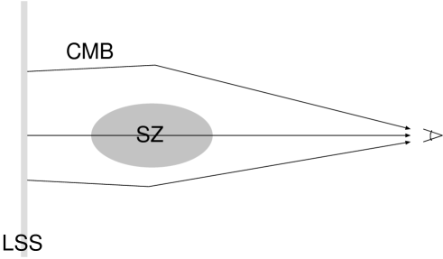
Figure 4.4: SZ–lensing Coupling

A schematic view of the SZ–lensing coupling bispectrum. One of the three CMB photons, which are decoupled at the last scattering surface (LSS), penetrates through a SZ cluster, changing its temperature, and coming toward us. As the other two photons pass through near the SZ cluster, they are deflected by the lensing effect, changing their propagation directions, and coming toward us. As a result, the three photons are correlated, generating three-point correlation, the bispectrum.

GS99 have derived $\left<\Theta^{*}_{lm}a_{lm}^{\rm SZ}\right>$, assuming the linear pressure bias model (PSCO95), $T_{\rho}=\overline{T}_{\rho}b_{\rm gas}\delta$, and the mean temperature evolution, $\overline{T}_{\rho}\simeq\overline{T}_{\rho 0}(1+z)^{-1}$, for $z<2$, which is roughly suggested by recent hydrodynamic simulations (CO99; RKSP00; SWH01). They have obtained

$$\left<\Theta^{*}_{lm}a_{lm}^{\rm SZ}\right>\simeq-j_{\nu}\frac{4y_{0}b_{\rm gas}l^{2}}{3\Omega_{\rm m}H_{0}^{2}}\int_{0}^{z_{*}}dz\frac{dr}{dz}D^{2}(z)(1+z)^{2}\frac{r_{*}-r(z)}{r_{*}^{2}r^{5}(z)}P_{\Phi}\left(k=\frac{l}{r(z)}\right),$$ (4.47)

where $D(z)$ is the linear growth factor. Simulations without non-gravitational heating (RKSP00; SWH01) suggest that $\overline{T}_{\rho 0}\sim 0.2-0.4~{}{\rm keV}$ and $b_{\rm gas}\sim 5-10$; analytic estimations give similar numbers (RKSP00; ZP01). In the pressure bias model, free parameters except cosmological parameters are $\overline{T}_{\rho 0}$ and $b_{\rm gas}$; however, both actually depend upon cosmological models (RKSP00). Since $l^{3}\left<\Theta^{*}_{lm}a_{lm}^{\rm SZ}\right>\sim 2\times 10^{-10}j_{\nu}\overline{T}_{\rho 0}b_{\rm gas}$ (GS99; CH00) and $l^{2}C_{l}^{\rm P}\sim 6\times 10^{-10}$, we have

$$b_{lll}^{\rm sz-lens}\sim l^{-3}\left[\left(l^{2}C_{l}^{\rm P}\right)\left(l^{3}\left<\Theta^{*}_{lm}a_{lm}^{\rm SZ}\right>\right)\times 5/2\right]\sim l^{-3}\times 3\times 10^{-19}j_{\nu}\overline{T}_{\rho 0}b_{\rm gas},$$ (4.48)

where $\overline{T}_{\rho 0}$ is in units of 1 keV, and $b_{l_{1}l_{2}l_{3}}=B_{l_{1}l_{2}l_{3}}^{m_{1}m_{2}m_{3}}\left({\cal G}_{l_{1}l_{2}l_{3}}^{m_{1}m_{2}m_{3}}\right)^{-1}$ is the reduced bispectrum (Eq.(4.9)). Comparing this with equation (4.27), we obtain

$$\frac{b_{lll}^{\rm primary}}{b_{lll}^{\rm sz-lens}}\sim l^{-1}\times 10\left(\frac{f_{\rm NL}}{j_{\nu}\overline{T}_{\rho 0}b_{\rm gas}}\right).$$ (4.49)

This estimate suggests that the SZ–lensing bispectrum overwhelms the primary bispectrum in small angular scales. This is why we have to separate the primary from the SZ–lensing effect.

While the pressure bias model gives a rough estimate of the SZ power spectrum, more accurate predictions exist. Several authors have predicted the SZ power spectrum analytically using the Press-Schechter approach (CK88; MS93; AM99; KK99; Coo00) or the hyper-extended perturbation theory (ZP01). The predictions agree with hydrodynamic simulations well (RKSP00; SBP01; SWH01; RT00; Kom01a). While a big uncertainty in the predictions has been lying in a phenomenological model which describes the SZ surface brightness profile of halos, KSel01 have proposed universal gas and temperature profiles, and predicted the SZ profile relying on the physical basis. Hence, using those universal profiles, one can improve the analytic prediction for the SZ power spectrum. We expect that the universal profiles describe the SZ profile in the average sense; on the individual halo-to-halo basis, there could be significant deviation from the universal profile, owing to substructures in halos (Kom01c).

4.3.2 Extragalactic radio and infrared sources

The bispectrum from extragalactic radio and infrared sources whose fluxes, $F$, are smaller than a certain detection threshold, $F_{\rm d}$, is simple to estimate, when we assume the Poisson distribution. tof98 have shown that the Poisson distribution is good approximation. The Poisson distribution has the white noise spectrum; thus, the reduced bispectrum (Eq.(4.9)) is constant, $b_{l_{1}l_{2}l_{3}}^{\rm ps}=b^{\rm ps}={\rm constant}$, and we obtain

$$B_{l_{1}l_{2}l_{3}}^{m_{1}m_{2}m_{3}}={\cal G}_{l_{l}1_{2}l_{3}}^{m_{1}m_{2}m_{3}}b^{\rm ps},$$ (4.50)

where

$$b^{\rm ps}(<F_{\rm d})\equiv g^{3}(x)\int_{0}^{F_{\rm d}}dFF^{3}\frac{dn}{dF}=g^{3}(x)\frac{n(>F_{\rm d})}{3-\beta}F_{\rm d}^{3}.$$ (4.51)

Here, $dn/dF$ is the differential source count per unit solid angle, and $n(>F_{\rm d})\equiv\int_{F_{\rm d}}^{\infty}dF(dn/dF)$. We have assumed a power-law count, $dn/dF\propto F^{-\beta-1}$, for $\beta<2$. The other symbols mean $x\equiv h\nu/k_{\rm B}T\simeq(\nu/56.80~{}{\rm GHz})(T/2.726~{}{\rm K})^{-1}$, and

$$g(x)\equiv 2\frac{(hc)^{2}}{(k_{\rm B}T)^{3}}\left(\frac{\sinh x/2}{x^{2}}\right)^{2}\simeq\frac{1}{67.55~{}{\rm MJy~{}sr^{-1}}}\left(\frac{T}{2.726~{}{\rm K}}\right)^{-3}\left(\frac{\sinh x/2}{x^{2}}\right)^{2}.$$ (4.52)

Using the Poisson angular power spectrum, $C^{\rm ps}$, given by

$$C^{\rm ps}(<F_{\rm d})\equiv g^{2}(x)\int_{0}^{F_{\rm d}}dFF^{2}\frac{dn}{dF}=g^{2}(x)\frac{n(>F_{\rm d})}{2-\beta}F_{\rm d}^{2},$$ (4.53)

we can rewrite $b^{\rm ps}$ into a different form,

$$b^{\rm ps}(<F_{\rm d})=\frac{(2-\beta)^{3/2}}{3-\beta}\left[n(>F_{\rm d})\right]^{-1/2}\left[C^{\rm ps}(<F_{\rm d})\right]^{3/2}.$$ (4.54)

tof98 have estimated $n(>F_{\rm d})\sim 300~{}{\rm sr^{-1}}$ for $F_{\rm d}\sim 0.2~{}{\rm Jy}$ at 217 GHz. This $F_{\rm d}$ corresponds to $5\sigma$ detection threshold for the Planck experiment at 217 GHz. RSH00 have extrapolated their estimation to 94 GHz, finding $n(>F_{\rm d})\sim 7~{}{\rm sr^{-1}}$ for $F_{\rm d}\sim 2~{}{\rm Jy}$, which corresponds to MAP $5\sigma$ threshold. These values yield

$$C^{\rm ps}(90~{}{\rm GHz},<2~{}{\rm Jy}) \sim 2\times 10^{-16},$$ (4.55)

$$C^{\rm ps}(217~{}{\rm GHz},<0.2~{}{\rm Jy}) \sim 1\times 10^{-17}.$$ (4.56)

Thus, rough estimates for $b^{\rm ps}$ are

$$b^{\rm ps}(90~{}{\rm GHz},<2~{}{\rm Jy}) \sim 2\times 10^{-25},$$ (4.57)

$$b^{\rm ps}(217~{}{\rm GHz},<0.2~{}{\rm Jy}) \sim 5\times 10^{-28}.$$ (4.58)

While we have assumed the Euclidean source count ($\beta=3/2$) for definiteness, this assumption does not affect an order of magnitude estimate here.

As the primary reduced bispectrum is $\propto l^{-4}$ (Eq.(4.27)), and the SZ–lensing reduced bispectrum is $\propto l^{-3}$ (Eq.(4.48)), the point-source bispectrum rapidly becomes to dominate the total bispectrum in small angular scales:

$$\frac{b_{lll}^{\rm primary}}{b^{\rm ps}} \sim l^{-4}\times 10^{7}\left(\frac{f_{\rm NL}}{b^{\rm ps}/10^{-25}}\right),$$ (4.59)

$$\frac{b_{lll}^{\rm sz-lens}}{b^{\rm ps}} \sim l^{-3}\times 10^{6}\left(\frac{j_{\nu}\overline{T}_{\rho 0}b_{\rm gas}}{b^{\rm ps}/10^{-25}}\right).$$ (4.60)

For example, the point sources overwhelm the SZ–lensing bispectrum measured by MAP at $l\lower 2.15277pt\hbox{$\;\buildrel>\over{\sim}\;$}100$.

What the SZ–lensing bispectrum and the point-source bispectrum look like? Figure 4.5 plots the primary, the SZ–lensing, and the point-source reduced bispecta for the equilateral configurations, $l\equiv l_{1}=l_{2}=l_{3}$. We have plotted $l^{2}(l+1)^{2}b_{lll}/(2\pi)^{2}$. We find that these bispecra are very different from each other in shape on small angular scales. It thus suggests that we can separate these three contributions on the basis of shape difference. We study this point in the next section.

Figure 4.5: Equilateral Reduced Bispectra

Comparison between the primary (solid line), the SZ–lensing (dashed line), and the point-source (dotted line) reduced bispectra for the equilateral configurations, $l\equiv l_{1}=l_{2}=l_{3}$. We have plotted $\left[l^{2}(l+1)^{2}b_{lll}/(2\pi)^{2}\right]\times 10^{16}$, which makes the Sachs–Wolfe plateau of the primary reduced bispectrum on large angular scales, $l\lower 1.93748pt\hbox{$\;\buildrel<\over{\sim}\;$}10$, easily seen.

4.4 Measuring Bispectra

4.4.1 Fisher matrix

In this section, we study how well we can measure the primary bispectrum, and how well we can separate it from the secondary bispectra. Suppose that we fit the observed bispectrum, $B_{l_{1}l_{2}l_{3}}^{\rm obs}$, by theoretically calculated bispectra, which include both the primary and secondary sources. We minimize $\chi^{2}$ defined by

$$\chi^{2}\equiv\sum_{2\leq l_{1}\leq l_{2}\leq l_{3}}\frac{\left(B_{l_{1}l_{2}l_{3}}^{\rm obs}-\sum_{i}A_{i}B^{(i)}_{l_{1}l_{2}l_{3}}\right)^{2}}{\sigma^{2}_{l_{1}l_{2}l_{3}}},$$ (4.61)

where $i$ denotes a component such as the primary, the SZ and lensing effects, extragalactic sources, and so on. We have removed unobservable modes, $l=0$ and $1$.

As we have shown in chapter 3, the variance of the bispectrum, $\sigma^{2}_{l_{1}l_{2}l_{3}}$, is the six-point function of $a_{lm}$ (Luo94; heavens98). When non-Gaussianity is weak, we calculate it as (SG99; GM00)

$$\sigma^{2}_{l_{1}l_{2}l_{3}}\equiv\left<B_{l_{1}l_{2}l_{3}}^{2}\right>-\left<B_{l_{1}l_{2}l_{3}}\right>^{2}\approx{\cal C}_{l_{1}}{\cal C}_{l_{2}}{\cal C}_{l_{3}}\Delta_{l_{1}l_{2}l_{3}},$$ (4.62)

where $\Delta_{l_{1}l_{2}l_{3}}$ takes values 1, 2, or 6 when all $l$’s are different, two are same, or all are same, respectively. ${\cal C}_{l}\equiv C_{l}+C_{l}^{\rm N}$ is the total CMB angular power spectrum, which includes the power spectrum of the detector noise, $C_{l}^{\rm N}$. We calculate $C_{l}^{\rm N}$ analytically following Knox95 with the noise characteristics of relevant experiments. We do not include $C_{l}$ from secondary sources, as they are subdominant compared with the primary $C_{l}$ and $C_{l}^{\rm N}$ for relevant experiments. Including $C_{l}$ from extragalactic sources (Eqs.(4.55) or (4.56)) changes our results less than 10%.

Taking $\partial\chi^{2}/\partial A_{i}=0$, we obtain normal equation,

$$\sum_{j}\left[\sum_{2\leq l_{1}\leq l_{2}\leq l_{3}}\frac{B_{l_{1}l_{2}l_{3}}^{(i)}B_{l_{1}l_{2}l_{3}}^{(j)}}{\sigma_{l_{1}l_{2}l_{3}}^{2}}\right]A_{j}=\sum_{2\leq l_{1}\leq l_{2}\leq l_{3}}\frac{B_{l_{1}l_{2}l_{3}}^{\rm obs}B_{l_{1}l_{2}l_{3}}^{(i)}}{\sigma_{l_{1}l_{2}l_{3}}^{2}}.$$ (4.63)

We then define the Fisher matrix, $F_{ij}$, as

$$F_{ij} \equiv \sum_{2\leq l_{1}\leq l_{2}\leq l_{3}}\frac{B_{l_{1}l_{2}l_{3}}^{(i)}B_{l_{1}l_{2}l_{3}}^{(j)}}{\sigma_{l_{1}l_{2}l_{3}}^{2}}$$ (4.66)

$$= \frac{2}{\pi}\sum_{2\leq l_{1}\leq l_{2}\leq l_{3}}\left(l_{1}+\frac{1}{2}\right)\left(l_{2}+\frac{1}{2}\right)\left(l_{3}+\frac{1}{2}\right)\left(\begin{array}[]{ccc}l_{1}&l_{2}&l_{3}\\ 0&0&0\end{array}\right)^{2}\frac{b_{l_{1}l_{2}l_{3}}^{(i)}b_{l_{1}l_{2}l_{3}}^{(j)}}{\sigma_{l_{1}l_{2}l_{3}}^{2}},$$

where we have used equation (4.10) to replace $B_{l_{1}l_{2}l_{3}}$ by the reduced bispectrum, $b_{l_{1}l_{2}l_{3}}$ (see Eq.(4.9) for definition). Since the covariance matrix of $A_{i}$ is $F_{ij}^{-1}$, we define the signal-to-noise ratio, $(S/N)_{i}$, for a component $i$, the correlation coefficient, $r_{ij}$, between different components $i$ and $j$, and the degradation parameter, $d_{i}$, of $(S/N)_{i}$ due to $r_{ij}$, as

$$\left(\frac{S}{N}\right)_{i} \equiv \frac{1}{\sqrt{F_{ii}^{-1}}},$$ (4.67)

$$r_{ij} \equiv \frac{F_{ij}^{-1}}{\sqrt{F^{-1}_{ii}F^{-1}_{jj}}},$$ (4.68)

$$d_{i} \equiv F_{ii}F_{ii}^{-1}.$$ (4.69)

Note that $r_{ij}$ does not depend upon the amplitude of bispectra, but the shape. We have defined $d_{i}$ so as $d_{i}=1$ for zero degradation, while $d_{i}>1$ for degraded $(S/N)_{i}$. SG99 and CH00 have considered the diagonal component of $F_{ij}^{-1}$. We study all the components to study the separatability between various bispectra.

We estimate an order of magnitude of $S/N$ as a function of a certain angular resolution, $l$, as follows. Since the number of modes contributing to $S/N$ increases as $l^{3/2}$, and $l^{3}\left(\begin{array}[]{ccc}l&l&l\\ 0&0&0\end{array}\right)^{2}\sim 0.36\times l$, we estimate $(S/N)_{i}\sim(F_{ii})^{1/2}$ as

$$\left(\frac{S}{N}\right)_{i}\sim\frac{1}{3\pi}l^{3/2}\times l^{3/2}\left|\left(\begin{array}[]{ccc}l&l&l\\ 0&0&0\end{array}\right)\right|\times\frac{l^{3}b_{lll}^{(i)}}{(l^{2}C_{l})^{3/2}}\sim l^{5}b_{lll}^{(i)}\times 4\times 10^{12},$$ (4.70)

where we have used $l^{2}C_{l}\sim 6\times 10^{-10}$.

Table 4.1 tabulates $F_{ij}$, while table 4.2 tabulates $F_{ij}^{-1}$; table 4.3 tabulates $(S/N)_{i}$, while table 4.4 tabulates $d_{i}$ in the diagonal, and $r_{ij}$ in the off-diagonal parts.

Table 4.1: Fisher Matrix

Fisher matrix, $F_{ij}$ (Eq.(4.66)). $i$ denotes a component in the first row; $j$ denotes a component in the first column. $\overline{T}_{\rho 0}$ is in units of 1 keV, $b^{\rm ps}_{25}\equiv b^{\rm ps}/10^{-25}$, and $b^{\rm ps}_{27}\equiv b^{\rm ps}/10^{-27}$.

COBE	primary	SZ–lensing	point sources
primary	$4.2\times 10^{-6}~{}f_{\rm NL}^{2}$	$-4.0\times 10^{-7}~{}f_{\rm NL}j_{\nu}\overline{T}_{\rho 0}b_{\rm gas}$	$-1.0\times 10^{-9}~{}f_{\rm NL}b^{\rm ps}_{25}$
SZ–lensing		$1.3\times 10^{-7}~{}(j_{\nu}\overline{T}_{\rho 0}b_{\rm gas})^{2}$	$3.1\times 10^{-10}~{}j_{\nu}\overline{T}_{\rho 0}b_{\rm gas}b^{\rm ps}_{25}$
point sources			$1.1\times 10^{-12}~{}(b^{\rm ps}_{25})^{2}$
MAP
primary	$3.4\times 10^{-3}~{}f_{\rm NL}^{2}$	$2.6\times 10^{-3}~{}f_{\rm NL}j_{\nu}\overline{T}_{\rho 0}b_{\rm gas}$	$2.4\times 10^{-3}~{}f_{\rm NL}b^{\rm ps}_{25}$
SZ–lensing		$0.14~{}(j_{\nu}\overline{T}_{\rho 0}b_{\rm gas})^{2}$	$0.31~{}j_{\nu}\overline{T}_{\rho 0}b_{\rm gas}b^{\rm ps}_{25}$
point sources			$5.6~{}(b^{\rm ps}_{25})^{2}$
Planck
primary	$3.8\times 10^{-2}~{}f_{\rm NL}^{2}$	$7.2\times 10^{-2}~{}f_{\rm NL}j_{\nu}\overline{T}_{\rho 0}b_{\rm gas}$	$1.6\times 10^{-2}~{}f_{\rm NL}b^{\rm ps}_{27}$
SZ–lensing		$39~{}(j_{\nu}\overline{T}_{\rho 0}b_{\rm gas})^{2}$	$5.7~{}j_{\nu}\overline{T}_{\rho 0}b_{\rm gas}b^{\rm ps}_{27}$
point sources			$2.7\times 10^{3}~{}(b^{\rm ps}_{27})^{2}$

Table 4.2: Inverted Fisher Matrix

Inverted Fisher matrix, $F_{ij}^{-1}$. The meaning of the symbols is the same as in table 4.1.

COBE	primary	SZ–lensing	point sources
primary	$3.5\times 10^{5}~{}f_{\rm NL}^{-2}$	$1.1\times 10^{6}~{}(f_{\rm NL}j_{\nu}\overline{T}_{\rho 0}b_{\rm gas})^{-1}$	$1.3\times 10^{7}~{}(f_{\rm NL}b^{\rm ps}_{25})^{-1}$
SZ–lensing		$3.1\times 10^{7}~{}(j_{\nu}\overline{T}_{\rho 0}b_{\rm gas})^{-2}$	$-7.8\times 10^{9}~{}(j_{\nu}\overline{T}_{\rho 0}b_{\rm gas}b^{\rm ps}_{25})^{-1}$
point sources			$3.1\times 10^{12}~{}(b^{\rm ps}_{25})^{-2}$
MAP
primary	$3.0\times 10^{2}~{}f_{\rm NL}^{-2}$	$-6.1~{}(f_{\rm NL}j_{\nu}\overline{T}_{\rho 0}b_{\rm gas})^{-1}$	$0.21~{}(f_{\rm NL}b^{\rm ps}_{25})^{-1}$
SZ–lensing		$8.4~{}(j_{\nu}\overline{T}_{\rho 0}b_{\rm gas})^{-2}$	$-0.46~{}(j_{\nu}\overline{T}_{\rho 0}b_{\rm gas}b^{\rm ps}_{25})^{-1}$
point sources			$0.21~{}(b^{\rm ps}_{25})^{-2}$
Planck
primary	$26~{}f_{\rm NL}^{-2}$	$-4.9\times 10^{-2}~{}(f_{\rm NL}j_{\nu}\overline{T}_{\rho 0}b_{\rm gas})^{-1}$	$-5.7\times 10^{-5}~{}(f_{\rm NL}b^{\rm ps}_{27})^{-1}$
SZ–lensing		$2.6\times 10^{-2}~{}(j_{\nu}\overline{T}_{\rho 0}b_{\rm gas})^{-2}$	$-5.4\times 10^{-5}~{}(j_{\nu}\overline{T}_{\rho 0}b_{\rm gas}b^{\rm ps}_{27})^{-1}$
point sources			$3.7\times 10^{-4}~{}(b^{\rm ps}_{27})^{-2}$

Table 4.3: Signal-to-noise Ratio

Signal-to-noise ratio, $(S/N)_{i}$ (Eq.(4.67)), of detecting the bispectrum. $i$ denotes a component in the first row. The meaning of the symbols is the same as in table 4.1.

	primary	SZ–lensing	point sources
COBE	$1.7\times 10^{-3}~{}f_{\rm NL}$	$1.8\times 10^{-4}~{}\left|j_{\nu}\right|\overline{T}_{\rho 0}b_{\rm gas}$	$5.7\times 10^{-7}~{}b_{25}^{\rm ps}$
MAP	$5.8\times 10^{-2}~{}f_{\rm NL}$	$0.34~{}\left|j_{\nu}\right|\overline{T}_{\rho 0}b_{\rm gas}$	$2.2~{}b_{25}^{\rm ps}$
Planck	$0.19~{}f_{\rm NL}$	$6.2~{}\left|j_{\nu}\right|\overline{T}_{\rho 0}b_{\rm gas}$	$52~{}b_{27}^{\rm ps}$

Table 4.4: Signal Degradation and Correlation Matrix

Signal degradation parameter, $d_{i}$ (Eq.(4.69)), and correlation coefficient, $r_{ij}$ (Eq.(4.68)), matrix. $i$ denotes a component in the first row; $j$ denotes a component in the first column. $d_{i}$ for $i=j$, while $r_{ij}$ for $i\neq j$.

COBE	primary	SZ–lensing	point sources
primary	$1.46$	$0.33~{}{\rm sgn}(j_{\nu})$	$1.6\times 10^{-2}$
SZ–lensing		$3.89$	$-0.79~{}{\rm sgn}(j_{\nu})$
point sources			$3.45$
MAP
primary	$1.01$	$-0.12~{}{\rm sgn}(j_{\nu})$	$2.7\times 10^{-2}$
SZ–lensing		$1.16$	$-0.35~{}{\rm sgn}(j_{\nu})$
point sources			$1.14$
Planck
primary	$1.00$	$-5.9\times 10^{-2}~{}{\rm sgn}(j_{\nu})$	$-5.8\times 10^{-4}$
SZ–lensing		$1.00$	$-1.8\times 10^{-2}~{}{\rm sgn}(j_{\nu})$
point sources			$1.00$

4.4.2 Measuring primary bispectrum

Figure 4.6 shows the signal-to-noise ratio, $S/N$. The top panel shows the differential $S/N$ for the primary bispectrum at $\ln l_{3}$ interval, $\left[d(S/N)^{2}/d\ln l_{3}\right]^{1/2}f_{\rm NL}^{-1}$, and the bottom panel shows the cumulative $S/N$, $(S/N)(<l_{3})f_{\rm NL}^{-1}$, which is $S/N$ summed up to a certain $l_{3}$. We have computed the detector noise power spectrum, $C_{l}^{\rm N}$, for COBE four-year map (Ben96), MAP 90 GHz channel, and Planck 217 GHz channel, and assumed full sky coverage. Figure 4.6 also shows the ideal experiment with no noise: $C_{l}^{\rm N}=0$. Both $\left[d(S/N)^{2}/d\ln l_{3}\right]^{1/2}$ and $(S/N)(<l_{3})$ increase monotonically with $l_{3}$, roughly $\propto l_{3}$, up to $l_{3}\sim 2000$ for the ideal experiment.

Figure 4.6: Signal-to-noise Ratio

The predictions of the signal-to-noise ratio, $S/N$, for COBE, MAP, and Planck experiments (see Eq.(4.67)). The differential $S/N$ at $\ln l_{3}$ interval is shown in the upper panel, while the cumulative $S/N$ up to a certain $l_{3}$ is shown in the bottom panel. Both are in units of $f_{\rm NL}$. Solid line represents the zero-noise ideal experiment, while dotted lines show the realistic experiments mentioned above. The total $(S/N)f^{-1}_{\rm NL}$ are $1.7\times 10^{-3}$, $5.8\times 10^{-2}$, and $0.19$ for COBE, MAP, and Planck experiments, respectively.

Beyond $l_{3}\sim 2000$, an enhancement of the damping tail in $C_{l}$ because of the weak lensing effect (Seljak96) stops $\left[d(S/N)^{2}/d\ln l_{3}\right]^{1/2}$, and hence $(S/N)(<l_{3})$, increasing. This leads to an important constraint on the observation; even for the ideal noise-free, infinitesimally thin beam experiment, there is an upper limit on the value of $S/N\lower 2.15277pt\hbox{$\;\buildrel<\over{\sim}\;$}0.3f_{\rm NL}$. For a given realistic experiment, $\left[d(S/N)^{2}/d\ln l_{3}\right]^{1/2}$ has a maximum at a scale near the beam size.

For COBE, MAP and Planck experiments, the total $(S/N)f^{-1}_{\rm NL}$ are $1.7\times 10^{-3}$, $5.8\times 10^{-2}$, and $0.19$, respectively (see table 4.3). To obtain $S/N>1$, we need $f_{\rm NL}>600$, 20, and $5$, while the ideal experiment requires $f_{\rm NL}>3$ (see table 4.5). We can also roughly obtain these values by substituting equation (4.27) into (4.70),

$$\left(\frac{S}{N}\right)_{\rm primary}\sim l\times 10^{-4}f_{\rm NL}.$$ (4.71)

The degradation parameters, $d_{\rm primary}$, are 1.46, 1.01, and 1.00 for COBE, MAP, and Planck experiments, respectively (see table 4.4), suggesting that MAP and Planck experiments will separate the primary bispectrum from the others with 1% or better accuracy; however, COBE cannot discriminate between them very well, as the primary and the secondary sources change monotonically on the COBE angular scales. On the MAP and Planck scales, the primary bispectrum starts oscillating around zero, being well separated in shape from the secondaries that do not oscillate. This is good news for the forthcoming high angular resolution CMB experiments.

4.4.3 Measuring secondary bispectra

Signal-to-noise ratios of detecting the SZ–lensing bispectrum, $(S/N)_{\rm sz-lens}$, in units of $\left|j_{\nu}\right|\overline{T}_{\rho 0}b_{\rm gas}$ are $1.8\times 10^{-4}$, 0.34, and 6.2 for COBE, MAP, and Planck experiments, respectively (see table 4.3), where $\overline{T}_{\rho 0}$ is in units of 1 keV. Using equations (4.70) and (4.48), we estimate $(S/N)_{\rm sz-lens}$ roughly as

$$\left(\frac{S}{N}\right)_{\rm sz-lens}\sim l^{2}\times 10^{-6}\left|j_{\nu}\right|\overline{T}_{\rho 0}b_{\rm gas}.$$ (4.72)

Hence, $(S/N)_{\rm sz-lens}$ increases with the angular resolution more rapidly than the primary bispectrum (see Eq.(4.71)). Since $\left|j_{\nu}\right|\overline{T}_{\rho 0}b_{\rm gas}$ should be of order unity, COBE and MAP cannot detect the SZ–lensing bispectrum; however, Planck is sensitive enough to detect, depending on the frequency, i.e., a value of $j_{\nu}$. For example, 217 GHz is insensitive to the SZ effect as $j_{\nu}\sim 0$, while $j_{\nu}=-2$ in the Rayleigh–Jeans regime.

The degradation parameters, $d_{\rm sz-lens}$, are 3.89, 1.16, and 1.00 for COBE, MAP, and Planck experiments, respectively (see table 4.4); thus, Planck will separate the SZ–lensing bispectrum from the other effects. Note that $(S/N)_{\rm sz-lens}$ values must be an order of magnitude estimation, for our cosmological model is the COBE normalized SCDM that yields $\sigma_{8}=1.2$, which is a factor of 2 greater than the cluster normalization for $\Omega_{\rm m}=1$, and $20\%$ greater than the normalization for $\Omega_{\rm m}=0.3$ (KS97). Hence, this factor tends to overestimate $\left<\Theta^{*}_{lm}a_{lm}^{\rm SZ}\right>$ (Eq.(4.47)) by a factor of less than 10; on the other hand, using the linear $P_{\Phi}(k)$ power spectrum rather than the non-linear power spectrum tends to underestimate the effect by a factor of less than 10 at $l\sim 3000$ (CH00). Yet, our main goal is to discriminate between the shapes of various bispectra, not to determine the amplitude, so that this factor does not affect our conclusion on the degradation parameters, $d_{i}$.

For the extragalactic radio and infrared sources, we estimate the signal-to-noise ratios as $5.7\times 10^{-7}(b^{\rm ps}/10^{-25})$, $2.2(b^{\rm ps}/10^{-25})$, and $52(b^{\rm ps}/10^{-27})$ for COBE, MAP, and Planck experiments, respectively (see table 4.3), and the degradation parameters, $d_{\rm ps}$, as 3.45, 1.14, and 1.00 (see table 4.4). Our estimate is consistent with RSH00. From equation (4.70), we find

$$\left(\frac{S}{N}\right)_{\rm ps}\sim l^{5}\times 10^{-13}\left(\frac{b^{\rm ps}}{10^{-25}}\right);$$ (4.73)

thus, $S/N$ of the point-source bispectrum increases very rapidly with the angular resolution.

Although MAP cannot separate the Poisson bispectrum from the SZ–lensing bispectrum very well (see $r_{ij}$ in table 4.4), the SZ–lensing bispectrum is too small to be measured by MAP anyway. Planck will do an excellent job on separating all kinds of bispectra, at least including the primary signal, SZ–lensing coupling, and extragalactic point sources, on the basis of the shape difference.

4.4.4 Measuring primary skewness

For the skewness, we define $S/N$ as

$$\left(\frac{S}{N}\right)^{2}\equiv\frac{S_{3}^{2}}{\sigma^{2}_{S_{3}}},$$ (4.74)

where the variance is (Srednicki93)

$$\sigma_{S_{3}}^{2} \equiv \left<\left(S_{3}\right)^{2}\right>=6\int_{-1}^{1}\frac{d\cos\theta}{2}\left[{\cal C}(\theta)\right]^{3}$$ (4.77)

$$= 6\sum_{l_{1}l_{2}l_{3}}\frac{\left(2l_{1}+1\right)\left(2l_{2}+1\right)\left(2l_{3}+1\right)}{(4\pi)^{3}}\left(\begin{array}[]{ccc}l_{1}&l_{2}&l_{3}\\ 0&0&0\end{array}\right)^{2}{\cal C}_{l_{1}}{\cal C}_{l_{2}}{\cal C}_{l_{3}}W^{2}_{l_{1}}W^{2}_{l_{2}}W^{2}_{l_{3}}$$

$$= \frac{9}{2\pi^{3}}\sum_{2\leq l_{1}\leq l_{2}\leq l_{3}}\left(l_{1}+\frac{1}{2}\right)\left(l_{2}+\frac{1}{2}\right)\left(l_{3}+\frac{1}{2}\right)\left(\begin{array}[]{ccc}l_{1}&l_{2}&l_{3}\\ 0&0&0\end{array}\right)^{2}$$ (4.81)

$$\times{\cal C}_{l_{1}}{\cal C}_{l_{2}}{\cal C}_{l_{3}}W^{2}_{l_{1}}W^{2}_{l_{2}}W^{2}_{l_{3}}.$$

In the last equality, we have used symmetry of the summed quantity with respect to indices (Eq.(4.39)), and removed unobservable modes, $l=0$ and $1$. Typically $\sigma_{S_{3}}\sim 10^{-15}$, as $\sigma_{S_{3}}\sim\left[{\cal C}(0)\right]^{3/2}\sim 10^{-15}$, where ${\cal C}(\theta)$ is the temperature auto correlation function including noise.

The bottom panel of figure 4.3 plots $\sigma_{S_{3}}(<l_{3})$, which is $\sigma_{S_{3}}$ summed up to a certain $l_{3}$, for COBE, MAP, and Planck experiments as well as for the ideal experiment. Since ${\cal C}_{l}W^{2}_{l}=C_{l}e^{-l(l+1)\sigma^{2}_{\rm b}}+w^{-1}$, where $w^{-1}$ is the white noise power spectrum of the detector noise (Knox95), $w^{-1}$ keeps $\sigma_{S_{3}}(<l_{3})$ slightly increasing with $l_{3}$ beyond the experimental angular resolution scale, $l\sim\sigma_{\rm b}^{-1}$. In contrast, $S_{3}(<l_{3})$ becomes constant beyond $l\sim\sigma_{\rm b}^{-1}$ (see the top panel of figure 4.3). As a result, $S/N$ starts slightly decreasing beyond the resolution. We use the maximum $S/N$ for calculating the minimum value of $f_{\rm NL}$ above which the primary $S_{3}$ is detectable; we find that $f_{\rm NL}>800$, 80, 70, and 60 for COBE, MAP, Planck, and the ideal experiments, respectively, assuming full sky coverage.

These $f_{\rm NL}$ values are systematically larger than those for detecting $B_{l_{1}l_{2}l_{3}}$ by a factor of 1.3, 4, 14, and 20, respectively (see table 4.5). The higher the angular resolution is, the less sensitive the primary $S_{3}$ is to non-Gaussianity than $B_{l_{1}l_{2}l_{3}}$. This is because the cancellation effect on smaller angular scales because of the oscillation of $B_{l_{1}l_{2}l_{3}}$ damps $S_{3}$.

4.5 Discussion and Conclusions

In this chapter, using the full radiation transfer function, we have numerically computed the primary cosmic microwave background bispectrum (Eq.(4.23)) and skewness (Eq.(4.38)) down to arcminutes angular scales. As the primary bispectrum oscillates around zero (figure 4.2), the primary skewness saturates at the MAP angular resolution scale, $l\sim 500$ (figure 4.3). We have introduced the reduced bispectrum, $b_{l_{1}l_{2}l_{3}}$, defined by equation (4.9), and found that this quantity is more useful to describe physical properties of the bispectrum than the angular averaged bispectrum, $B_{l_{1}l_{2}l_{3}}$ (Eq.(4.3)).

Figure 4.7 compares the expected signal-to-noise ratio of detecting the primary non-Gaussianity based on the bispectrum (Eq.(4.67)) with that based on the skewness (Eq.(4.74)). It shows that the bispectrum is almost an order of magnitude more sensitive to the non-Gaussianity than the skewness. We conclude that when we can compute the predicted form of the bispectrum, it becomes a “matched filter” for detecting the non-Gaussianity in data, and thus much more powerful tool than the skewness. Table 4.5 summarizes the minimum $f_{\rm NL}$ for detecting the primary non-Gaussianity using the bispectrum or the skewness for COBE, MAP, Planck, and the ideal experiments. This shows that even the ideal experiment needs $f_{\rm NL}>3$ to detect the primary bispectrum.

Figure 4.7: Bispectrum vs Skewness

Comparison of the signal-to-noise ratio summed up to a certain $l_{3}$, $S/N(<l_{3})$, for the bispectrum (top panel; Eq.(4.67)) and the skewness (bottom panel; Eq.(4.74)). $S/N(<l_{3})$ is in units of $f_{\rm NL}$. The dotted lines show COBE, MAP, and Planck experiments (dotted lines), while the solid line shows the ideal experiment. See table 4.5 for $f_{\rm NL}$ to obtain $S/N>1$.

Table 4.5: Detection Limit for the Non-linear Coupling Parameter

The minimum non-linear coupling parameter, $f_{\rm NL}$, needed for detecting the primary non-Gaussianity by the bispectrum or the skewness with the signal-to-noise ratio greater than 1. These estimates include the effects of cosmic variance, detector noise, and foreground sources.

Experiments	$f_{\rm NL}$ (Bispectrum)	$f_{\rm NL}$ (Skewness)
COBE	600	800
MAP	20	80
Planck	5	70
Ideal	3	60

We have calculated the secondary bispectra from the coupling between the SZ effect and the weak lensing effect, and from the extragalactic radio and infrared sources. Only Planck will detect the SZ–lensing bispectrum, while both MAP and Planck will detect the extragalactic point-source bispectrum (table 4.3).

We have also studied how well we can discriminate between the primary, the SZ–lensing coupling, and the extragalactic point-source bispectra. We have found that MAP and Planck will separate the primary from the other secondary sources with 1% or better accuracy. This conclusion is due to the acoustic oscillation in the primary bispectrum that does not appear in the secondary bispectra. The SZ–lensing coupling and the extragalactic sources are well separately measured by Planck experiment, although COBE and MAP cannot discriminate between them (table 4.4).

Our arguments on the ability to discriminate between various bispectra have been based upon the shape difference, and thus have not taken into account the spectral difference in frequency space. TE96 and CHT00 have shown that the multi-band observation is efficient for discriminating between the primary signal and the other foreground sources in the CMB power spectrum. Their scheme should be effective on the bispectrum as well, and will improve the accuracy of the foreground removal further. We thus expect that MAP and Planck will measure the primary bispectrum separately from the foregrounds.

Simple slowly-rolling single-field inflation models predict $f_{\rm NL}\sim{\cal O}(10^{-2})$ (SB90; SB91; Gan94), while the second order perturbation theory predicts $f_{\rm NL}\sim{\cal O}(1)$ (PC96); thus, significant detection of the primary bispectrum or the skewness with any experiments means that these inflation models need to be modified. According to our results, if the reported detection (FMG98; Mag00) of the bispectrum on the COBE map were cosmological in origin, then MAP and Planck would detect the primary bispectrum much more significantly. While Banday, Zaroubi and Górski (BZG00) have shown that the one of those detections (FMG98) is accounted for by the experimental systematic effects, the other (Mag00) is significant even after removing such the systematics.

Although we have not discussed so far, spatial distribution of interstellar dust emissions is a potential source of microwave non-Gaussianity. While it is very hard to estimate the bispectrum analytically, we can use the dust template map compiled by SFD98 to estimate the dust bispectrum. For example, we have found that the dimensionless skewness parameter, $\left<(\Delta T)^{3}\right>/\left<(\Delta T)^{2}\right>^{3/2}$, is as large as 51 on the template map. We have used the publicly available HEALPix-formatted (GHW98) $100~{}\mu{\rm m}$ map, which contains 12,582,912 pixels without sky-cut. The mean intensity in the map is $14.8~{}{\rm MJy~{}sr^{-1}}$. Of course, this skewness is largely an overestimate for the real CMB measurement; we need to cut a fraction of the sky that contains the Galactic plane, and this will greatly reduce the non-Gaussianity. Nevertheless, residual non-Gaussianity is still a source of the microwave bispectrum, and has to be taken into account. Moreover, the form of the measured bispectrum on the dust map reflects the physics of interstellar dust, which is highly uncertain at present; thus, studying the interstellar dust bispectrum is a challenging field.

Chapter 5 Measurement of Bispectrum on the COBE DMR sky maps

Several authors have attempted to measure non-Gaussianity in CMB using various statistical techniques (e.g., Kogut et al. 1996b); as yet no conclusive detection has been reported except for measurement of several modes of the normalized CMB bispectrum on the COBE Differential Microwave Radiometer (DMR) sky maps (FMG98; Mag00). The existence of non-Gaussianity in the DMR data is controversial. If the CMB sky were non-Gaussian, this would challenge our simplest inflationary model.

The angular bispectrum, $B_{l_{1}l_{2}l_{3}}$, is the harmonic transform of the three-point correlation function. We carefully distinguish the normalized bispectrum, $B_{l_{1}l_{2}l_{3}}/\left(C_{l_{1}}C_{l_{2}}C_{l_{3}}\right)^{1/2}$, from the bispectrum, $B_{l_{1}l_{2}l_{3}}$. FMG98 have measured 9 equilateral ($l_{1}=l_{2}=l_{3}$) modes of the normalized bispectrum, $B_{l_{1}l_{2}l_{3}}/\left(C_{l_{1}}C_{l_{2}}C_{l_{3}}\right)^{1/2}$, on the DMR map, claiming detection at $l_{1}=l_{2}=l_{3}=16$. Their result has been under extensive efforts to confirm its significance and origin. BT99 claim that a few individual pixels in the DMR map are responsible for the most of the signal. BZG00 have proposed an eclipse effect by the Earth against the COBE satellite as a possible source of the signal. Mag00 has measured other 8 inter-$l$ modes of the normalized bispectrum such as $B_{l-1ll+1}/\left(C_{l-1}C_{l}C_{l+1}\right)^{1/2}$, and claims that scatter of the normalized bispectrum among 8 modes is too small to be consistent with Gaussian. SM00 further report measurement of 24 other inter-$l$ modes for different lags in $l$, and conclude they are consistent with Gaussian.

Thus, until now 41 modes of the normalized bispectrum have been measured on the DMR map. Here, we simply ask: “how many modes are available in the DMR map for the bispectrum?” The answer is 466, up to a maximum multipole of 20 that corresponds to the DMR beam size; thus, it is conceivable that the claimed detection of the normalized bispectrum at $l_{1}=l_{2}=l_{3}=16$ would be explained by a statistical fluctuation, as 9 modes are expected to have statistical significance above 98% out of 466 independent modes even if CMB is exactly Gaussian. In this chapter, we measure 466 modes of the CMB bispectrum on the COBE DMR sky maps, testing the claimed detection of the bispectrum and non-Gaussianity. We take into account the covariance between these modes due to the Galactic cut, which has not been done in the previous work.

On the theoretical side, several predictions for the CMB bispectrum exist. Several authors (FRS93; LS93; Gan94) have predicted the primary bispectrum (or equivalently three-point correlation function) on the DMR angular scales from slow-roll inflation models. In chapter 4, we have extended the prediction down to arcminutes scales using the full radiation transfer function.

In addition to the primary one, secondary sources in the low-redshift universe and foreground sources produce the bispectrum through their non-linearity. LS93 and SG99 have calculated the secondary bispectrum arising from non-linear evolution of gravitational potential; GS99 and CH00 have calculated the one from the gravitational lensing effect coupled with various secondary anisotropy sources. In chapter 4, we have calculated the foreground bispectrum from extragalactic radio and infrared point sources. While the bispectrum is not the best tool for detecting the signature of rare highly non-linear events, e.g., textures (PK01), it is sensitive to weakly non-linear effects.

Having theoretical predictions is a great advantage in extracting physical information from measurement; one can fit a predicted bispectrum to the data so as to constrain parameters in a theory. Since the DMR beam size is large enough to minimize contribution from the secondary and the extragalactic foreground sources, the only relevant source would be the primary one. In this chapter, we fit a theoretical primary bispectrum (KS01a) to the data.

The Galactic plane contains strong microwave emissions from interstellar sources. The emissions are highly non-Gaussian, and distributed on fairly large angular scales. Unfortunately, predicting the CMB bispectrum from interstellar sources is very difficult; thus, we excise the galactic plane from the DMR data. We model the residual foreground bispectrum at high galactic latitude using foreground template maps. By simultaneously fitting the foreground bispectrum and the primary bispectrum to the DMR data for three different Galactic cuts, we quantify the importance of the interstellar emissions in our analysis.

This chapter is organized as follows. In § 5.1, we define the angular bispectrum, and show how to compute it efficiently from observational data. In § 5.2, we study statistical properties of the bispectrum and the normalized bispectrum. We then measure the normalized bispectrum from the COBE DMR four-year sky maps (Ben96), testing Gaussianity of the DMR map. In § 5.3, we fit predicted bispectra to the DMR data, constraining parameters in the predictions. The predictions include the primary bispectrum from inflation and the foreground bispectrum from interstellar Galactic emissions. Finally, § 5.4 concludes.

5.1 Angular Bispectrum

The CMB angular bispectrum consists of a product of three harmonic transforms of the CMB temperature field. For Gaussian fields, expectation value of the bispectrum is exactly zero. Given statistical isotropy of the universe, the angular averaged bispectrum, $B_{l_{1}l_{2}l_{3}}$, is given by

$$B_{l_{1}l_{2}l_{3}}=\sum_{{\rm all}~{}m}\left(\begin{array}[]{ccc}l_{1}&l_{2}&l_{3}\\ m_{1}&m_{2}&m_{3}\end{array}\right)a_{l_{1}m_{1}}a_{l_{2}m_{2}}a_{l_{3}m_{3}},$$ (5.1)

where the matrix denotes the Wigner-$3j$ symbol, and harmonic coefficients, $a_{lm}$, are given by

$$a_{lm}=\int_{\Omega_{\rm obs}}d^{2}\hat{\mathbf{n}}~{}\frac{\Delta T\left(\hat{\mathbf{n}}\right)}{T}Y_{lm}^{*}\left(\hat{\mathbf{n}}\right).$$ (5.2)

$\Omega_{\rm obs}$ denotes a solid angle of the observed sky. $B_{l_{1}l_{2}l_{3}}$ satisfies the triangle condition, $\left|l_{i}-l_{j}\right|\leq l_{k}\leq l_{i}+l_{j}$ for all permutations of indices, and parity invariance, $l_{1}+l_{2}+l_{3}={\rm even}$.

We can rewrite equation (5.1) into a more useful form. Using the identity,

$$\left(\begin{array}[]{ccc}l_{1}&l_{2}&l_{3}\\ m_{1}&m_{2}&m_{3}\end{array}\right) = \left(\begin{array}[]{ccc}l_{1}&l_{2}&l_{3}\\ 0&0&0\end{array}\right)^{-1}\sqrt{\frac{(4\pi)^{3}}{\left(2l_{1}+1\right)\left(2l_{2}+1\right)\left(2l_{3}+1\right)}}$$ (5.8)

$$\times\int\frac{d^{2}\hat{\mathbf{n}}}{4\pi}~{}Y_{l_{1}m_{1}}(\hat{\mathbf{n}})Y_{l_{2}m_{2}}(\hat{\mathbf{n}})Y_{l_{3}m_{3}}(\hat{\mathbf{n}}),$$

we rewrite equation (5.1) as

$$B_{l_{1}l_{2}l_{3}}=\left(\begin{array}[]{ccc}l_{1}&l_{2}&l_{3}\\ 0&0&0\end{array}\right)^{-1}\int\frac{d^{2}\hat{\mathbf{n}}}{4\pi}~{}e_{l_{1}}(\hat{\mathbf{n}})e_{l_{2}}(\hat{\mathbf{n}})e_{l_{3}}(\hat{\mathbf{n}}),$$ (5.9)

where the integral is not over $\Omega_{\rm obs}$, but over the whole sky; $e_{l}(\hat{\mathbf{n}})$ already encapsulates the information of incomplete sky coverage through $a_{lm}$. Following chapter 3, we used the azimuthally averaged harmonic transform of the CMB temperature field, $e_{l}(\hat{\mathbf{n}})$,

$$e_{l}(\hat{\mathbf{n}})=\sqrt{\frac{4\pi}{2l+1}}\sum_{m}a_{lm}Y_{lm}(\hat{\mathbf{n}}).$$ (5.10)

Similarly, we write the angular power spectrum, $C_{l}$, as

$$C_{l}=\int\frac{d^{2}\hat{\mathbf{n}}}{4\pi}~{}e^{2}_{l}(\hat{\mathbf{n}}).$$ (5.11)

Thus, $e_{l}(\hat{\mathbf{n}})$ is a square-root of $C_{l}$ at a given position of the sky. Equation (5.9) is computationally efficient, as we can calculate $e_{l}(\hat{\mathbf{n}})$ quickly with the spherical harmonic transform for a given $l$. Since the HEALPix pixels have the equal area (GHW98), the average over the whole sky, $\int d^{2}\hat{\mathbf{n}}/(4\pi)$, is done by the sum over all pixels divided by the total number of pixels, $N^{-1}\sum_{i}^{N}$.

5.2 Measurement of Bispectrum on the DMR Sky Maps

5.2.1 The data

We use the HEALPix-formatted (GHW98) COBE DMR four-year sky map, which contains 12,288 pixels in Galactic coordinate with a pixel size $1.^{\circ}83$. We obtain the most sensitive sky map to CMB by combining 53 GHz map with 90 GHz map, after coadding the channels A and B at each frequency. We do not subtract eclipse season time-ordered data; while BZG00 ascribe the reported non-Gaussianity to this data, we will argue in this paper that the claimed detection of the normalized bispectrum at $l_{1}=l_{2}=l_{3}=16$ (FMG98) can also be explained in terms of a statistical fluctuation.

We reduce interstellar Galactic emissions by using three different Galactic cuts: $20^{\circ}$, $25^{\circ}$, and $30^{\circ}$ in Galactic latitude. Since we want to see how the different Galactic cuts affect the measured bispectrum, we use the three different Galactic cuts instead of the extended Galactic cut (Ban97), which is commonly used for analyzing the DMR sky maps. Then, we subtract the monopole and the dipole from each cut map, minimizing contaminations from these two multipoles to higher order multipoles through the mode-mode coupling. The coupling arises from incomplete sky coverage. This is very important to do, for the leakage of power from the monopole and the dipole to the higher order multipoles is rather big. We use the least-squares fit weighted by the pixel noise variance to measure the monopole and the dipole on each cut map. Table 5.1 shows the amplitude of the subtracted monopole and the dipole for the different Galactic cuts.

Table 5.1: Monopole and Dipole Subtraction

The monopole, $T_{0}$, and the dipole, $T_{1}$, anisotropies that have been subtracted from the DMR sky maps. We show the subtracted values for zero, $20^{\circ}$, $25^{\circ}$, and $30^{\circ}$ cuts. The rightmost column shows the directions of the subtracted dipole in Galactic coordinate.

$\left|b_{\rm cut}\right|$	${T}_{0}$ [$\mu$K]	${T}_{1}$ [$\mu$K]	${\mathbf{T}}_{1}/{T}_{1}$ ($l,b$)
$0^{\circ}$	1.40	63.1	($28.^{\circ}07$, $2.^{\circ}12$)
$20^{\circ}$	$-70.3$	26.2	($89.^{\circ}23$, $-4.^{\circ}17$)
$25^{\circ}$	$-72.4$	26.9	($84.^{\circ}89$, $-5.^{\circ}13$)
$30^{\circ}$	$-73.4$	28.6	($97.^{\circ}32$, $-6.^{\circ}31$)

We measure the bispectrum, $B_{l_{1}l_{2}l_{3}}$, on the DMR sky maps as follows. First, we measure $a_{lm}$ using equation (5.2). Then, we transform $a_{lm}$ for $-l\leq m\leq l$ into $e_{l}(\hat{\mathbf{n}})$ through equation (5.10). Finally, we obtain $B_{l_{1}l_{2}l_{3}}$ from equation (5.9), arranging $l_{1}$, $l_{2}$, and $l_{3}$ in order of $l_{1}\leq l_{2}\leq l_{3}$, where the maximum $l_{3}$ is set to be 20. In total, we have 466 non-zero modes after taking into account $\left|l_{i}-l_{j}\right|\leq l_{k}\leq l_{i}+l_{j}$ and $l_{1}+l_{2}+l_{3}={\rm even}$. Measurement of 466 modes takes about 1 second of CPU time on a Pentium-III single processor personal computer.

5.2.2 Monte–Carlo Simulations

We use Monte–Carlo simulations to estimate the covariance matrix of the measured bispectrum. Our simulation includes (a) a Gaussian random realization of the primary CMB anisotropy field drawn from the COBE-normalized ${\Lambda}$CDM power spectrum, and (b) a Gaussian random realization of the instrumental noise drawn from diagonal terms of the COBE DMR noise covariance matrix (Lin94). For computational efficiency, we do not use off-diagonal terms as they are smaller than 1% of the diagonal terms (Lin94).

We generate the input power spectrum, $C_{l}$, using the CMBFAST code (SZ96) with cosmological parameters fixed at $\Omega_{\rm cdm}=0.25$, $\Omega_{\Lambda}=0.7$, $\Omega_{\rm b}=0.05$, $h=0.7$, and $n=1$; the CMBFAST code uses the BW97 normalization.

In each realization, we generate $a_{lm}$ from the power spectrum, multiply it by the harmonic-transformed DMR beam, $G_{l}$ (Wri94), transform $G_{l}a_{lm}$ back to a sky map, and add an instrumental noise realization to the map. Finally, we measure 466 modes of the bispectrum from each realization. We generate 50,000 realizations for one simulation; processing one realization takes about 1 second, so that one simulation takes about 16 hours of CPU time on a Pentium-III single processor personal computer.

5.2.3 Normalized bispectrum

The input power spectrum determines the variance of the bispectrum. Off-diagonal terms in the covariance matrix arise from incomplete sky coverage. When non-Gaussianity is weak, the variance is given by (Luo94; heavens98; SG99; GM00)

$$\left<B_{l_{1}l_{2}l_{3}}^{2}\right>=\left<C_{l_{1}}\right>\left<C_{l_{2}}\right>\left<C_{l_{3}}\right>\Delta_{l_{1}l_{2}l_{3}},$$ (5.12)

where $\Delta_{l_{1}l_{2}l_{3}}$ takes values 1, 2, or 6 for all $l$’s are different, two are same, or all are same, respectively. The brackets denote the ensemble average.

The variance is undesirably sensitive to the input power spectrum; even if the input power spectrum were slightly different from the true power spectrum on the DMR map, the estimated variance from simulations would be significantly wrong, and we would erroneously conclude that the DMR map is inconsistent with Gaussian. It is thus not a robust test of Gaussianity to compare the measured bispectrum with the Monte–Carlo simulations.

The normalized bispectrum, $B_{l_{1}l_{2}l_{3}}/\left(C_{l_{1}}C_{l_{2}}C_{l_{3}}\right)^{1/2}$, is more sensible quantity than the bare bispectrum. Mag95 shows that the normalized bispectrum is a rotationally invariant spectrum independent of the power spectrum, as it factors out fluctuation amplitude in $a_{lm}$, which is measured by $C_{l}^{1/2}$. By construction, the variance of the normalized bispectrum is insensitive to the power spectrum, approximately given by $\Delta_{l_{1}l_{2}l_{3}}$.

One might wonder if the normalized bispectrum is too noisy to be useful, as the power spectrum in the denominator is also uncertain to some extent; however, we find that the variance is actually slightly smaller than $\Delta_{l_{1}l_{2}l_{3}}$. Figure 5.1 compares the variance of the normalized bispectrum, $\left<B_{l_{1}l_{2}l_{3}}^{2}/\left(C_{l_{1}}C_{l_{2}}C_{l_{3}}\right)\right>$, with that of the bispectrum, $\left<B_{l_{1}l_{2}l_{3}}^{2}\right>/\left(\left<C_{l_{1}}\right>\left<C_{l_{2}}\right>\left<C_{l_{3}}\right>\right)$. The top-left panel shows the case of full sky coverage. We find that the variance of the normalized bispectrum is precisely 1 when all $l$’s are different, while it is slightly smaller than 2 or 6 when two $l$’s are same or all $l$’s are same, respectively. This arises due to correlation between the uncertainties in the bispectrum and the power spectrum, and this correlation tends to reduce the total variance of the normalized bispectrum. The rest of panels show the cases of incomplete sky coverage. While the variance becomes more scattered than the case of full sky coverage, the variance of the normalized bispectrum is still systematically smaller than that of the bare bispectrum. Thus, the normalized bispectrum is reasonably sensitive to non-Gaussianity, yet it is not sensitive to the overall normalization of power spectrum.

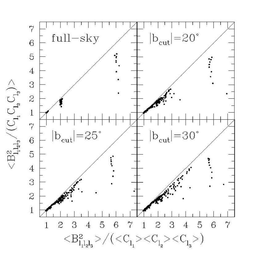
Figure 5.1: Variance of Normalized Bispectrum and Bare Bispectrum

Variance of the normalized bispectrum, $\left<B_{l_{1}l_{2}l_{3}}^{2}/\left(C_{l_{1}}C_{l_{2}}C_{l_{3}}\right)\right>$, in comparison with variance of the bare bispectrum, $\left<B_{l_{1}l_{2}l_{3}}^{2}\right>/\left(\left<C_{l_{1}}\right>\left<C_{l_{2}}\right>\left<C_{l_{3}}\right>\right)$. These are derived from simulated realizations of a Gaussian sky. The top-left panel shows the case of full sky coverage, while the rest of panels show the cases of incomplete sky coverage. The top-right, bottom-left, and bottom-right panels use the $20^{\circ}$, $25^{\circ}$, and $30^{\circ}$ Galactic cuts, respectively.

What distribution does the normalized bispectrum obey for a Gaussian field? First, even for a Gaussian field, the probability distribution of a single mode of $B_{l_{1}l_{2}l_{3}}$ is non-Gaussian, characterized by a large kurtosis. Figure 5.2 plots the distributions of 9 modes of $B_{l_{1}l_{2}l_{3}}$ drawn from the Monte–Carlo simulations (solid lines) in comparison with Gaussian distributions calculated from r.m.s. values (dashed lines). We find that the distribution does not fit the Gaussian very well. Then, we examine distribution of the normalized bispectrum, $B_{l_{1}l_{2}l_{3}}/\left(C_{l_{1}}C_{l_{2}}C_{l_{3}}\right)^{1/2}$. We find that the distribution is very much Gaussian except for $l_{1}=l_{2}=l_{3}=2$. Figure 5.3 plots the distributions of the 9 modes of the normalized bispectrum (solid lines) in comparison with Gaussian distributions calculated from r.m.s. values (dashed lines). The distribution fits the Gaussian remarkably well; this motivates our using standard statistical methods developed for Gaussian fields to analyze the normalized bispectrum. We could not make this simplification if we were analyzing the bare bispectrum. Furthermore, the central limit theorem implies that when we combine 466 modes the deviation of the distribution from Gaussianity becomes even smaller.

Figure 5.2: Distribution of Bispectrum

Distribution of the bare bispectrum drawn from the Monte–Carlo simulations (solid lines). The $20^{\circ}$ Galactic cut is used. $B_{l_{1}l_{2}l_{3}}/\left(\left<C_{l_{1}}\right>\left<C_{l_{2}}\right>\left<C_{l_{3}}\right>\right)^{1/2}$ is plotted, where the brackets denote the ensemble average over realizations from the Monte–Carlo simulations. The dashed lines plot Gaussian distributions calculated from r.m.s. values. Each panel represents a certain mode of $(l_{1},l_{2},l_{3})$ as quoted in the panels.

Figure 5.3: Distribution of Normalized Bispectrum

Distribution of the normalized bispectrum (solid lines), $B_{l_{1}l_{2}l_{3}}/\left(C_{l_{1}}C_{l_{2}}C_{l_{3}}\right)^{1/2}$, in comparison with Gaussian distributions calculated from r.m.s. values (dashed lines). The $20^{\circ}$ Galactic cut is used. The meaning of the panels is the same as in figure 5.2.

FMG98 claim detection of the normalized bispectrum at $l_{1}=l_{2}=l_{3}=16$; Mag00 claims that the scatter of the normalized bispectrum for $l_{1}=l_{2}-1$ and $l_{3}=l_{2}+1$ is too small to be consistent with Gaussian. The former has analyzed 9 modes, while the latter has analyzed 8 modes. In the next section, we analyze 466 modes, testing the statistical significance of the non-Gaussianity with much more samples than the previous work. We calculate $C_{l}$ from equation (5.11), and then divide $B_{l_{1}l_{2}l_{3}}$ by $\left(C_{l_{1}}C_{l_{2}}C_{l_{3}}\right)^{1/2}$ to obtain the normalized bispectrum.

5.2.4 Testing Gaussianity of the DMR map

We characterize statistical significance of the normalized bispectrum as probability of the measured normalized bispectrum being greater than those drawn from the Monte–Carlo simulations. We define the probability $P$ as

$$P_{\alpha}\equiv\frac{N\left(\left|I_{\alpha}^{\rm DMR}\right|>\left|I_{\alpha}^{\rm MC}\right|\right)}{N_{\rm total}}=\int_{-\left|I_{\alpha}^{\rm DMR}\right|}^{\left|I_{\alpha}^{\rm DMR}\right|}dx~{}F_{\alpha}^{\rm MC}(x),$$ (5.13)

where $I_{\alpha}$ is the normalized bispectrum, $N_{\rm total}=50,000$ is the total number of simulated realizations, and $\alpha=$ 1, 2, 3, 4,…, 466 represent $(l_{1},l_{2},l_{3})=$ (2,2,2), (2,3,3), (2,2,4), (3,3,4),…, (20,20,20), respectively, with satisfying $l_{1}\leq l_{2}\leq l_{3}$, $\left|l_{i}-l_{j}\right|\leq l_{k}\leq l_{i}+l_{j}$, and $l_{1}+l_{2}+l_{3}={\rm even}$. $F_{\alpha}^{\rm MC}(x)$ is the probability density distribution function (p.d.f) of the simulated realizations for the normalized bispectrum, $x=I_{\alpha}^{\rm MC}$. The p.d.f is normalized to unity: $\int_{-\infty}^{\infty}dxF_{\alpha}^{\rm MC}(x)=1$; thus, $P_{\alpha}$ lies in $0\leq P_{\alpha}\leq 1$.

By construction, the distribution of $P_{\alpha}$ is uniform, if the DMR map is consistent with the simulated realizations, i.e., Gaussian. We give the proof as follows. By rewriting equation (5.13) as $P_{\alpha}=f(\left|I_{\alpha}^{\rm DMR}\right|)$, we calculate the p.d.f of $P_{\alpha}$, $G(P_{\alpha})$, as

$$G(P_{\alpha}) = \int_{-\infty}^{\infty}dy~{}\delta\left[P_{\alpha}=f(\left|y\right|)\right]F_{\alpha}^{\rm DMR}(y)$$ (5.14)

$$= \int_{0}^{\infty}dy~{}\delta\left[P_{\alpha}=f(y)\right]\left[F_{\alpha}^{\rm DMR}(y)+F_{\alpha}^{\rm DMR}(-y)\right]$$

$$= \int_{0}^{\infty}dy~{}\frac{\delta\left[y=f^{-1}(P_{\alpha})\right]}{df/dy}\left[F_{\alpha}^{\rm DMR}(y)+F_{\alpha}^{\rm DMR}(-y)\right]$$

$$= \int_{0}^{\infty}dy~{}\delta\left[y=f^{-1}(P_{\alpha})\right]\frac{F_{\alpha}^{\rm DMR}(y)+F_{\alpha}^{\rm DMR}(-y)}{F^{\rm MC}_{\alpha}(y)+F^{\rm MC}_{\alpha}(-y)},$$

where $F_{\alpha}^{\rm DMR}(y)$ is the p.d.f of the measured normalized bispectrum on the DMR map, $y=I_{\alpha}^{\rm DMR}$. Our goal is to see if $F_{\alpha}^{\rm DMR}(y)$ is consistent with the DMR data being Gaussian. It follows from equation (5.14) that $G(P_{\alpha})\equiv 1$, when $F_{\alpha}^{\rm DMR}(y)\equiv F^{\rm MC}_{\alpha}(y)$, regardless of the functional form of $F^{\rm MC}_{\alpha}(y)$. In other words, the distribution of $P_{\alpha}$ is uniform, if the distribution of the measured normalized bispectrum is the same as the simulated realizations. Since our simulation assumes the DMR map Gaussian, the $P$ distribution, $G(P)$, tests the Gaussianity of the DMR map. If the $P$ distribution is not uniform, then we conclude the DMR data to be non-Gaussian.

A Gaussian field gives equal number of modes in each bin of $P$. For example, it gives 46.6 modes in $\Delta P=10\%$ bin: $466\times G(P)\Delta P=466\times 0.1=46.6$. If we detect the normalized bispectrum significantly, then we find that $G(P)$ is not uniform, but increases rapidly as $P$ increases.

The top panel of figure 5.4 plots the $P$ distribution for the three different Galactic cuts. We find that the distribution is uniform, and the number of modes in the bin ($\Delta P=10\%$) is consistent with the expectation value for Gaussian fluctuations (46.6).

Figure 5.4: KS Test for Gaussianity with Bispectrum

$P$ distribution (Eq.(5.13)). $P$ is the probability of the CMB normalized bispectrum, $B_{l_{1}l_{2}l_{3}}/\left(C_{l_{1}}C_{l_{2}}C_{l_{3}}\right)^{1/2}$, measured on the COBE DMR $53+90~{}{\rm GHz}$ sky map, being larger than those drawn from the Monte–Carlo simulations. There are 466 modes in total. The thick dashed, solid, and dotted lines represent the three different Galactic cuts as quoted in the figure. The thin solid line shows the expectation value for a Gaussian field. The top panel shows the $P$ distribution, while the bottom panel shows the cumulative $P$ distribution, for which we calculate the KS statistic. The KS statistic gives the probability of the distribution being consistent with the expectation for Gaussianity as 6.7%, 77%, and 52% for the three Galactic cuts, respectively.

To further quantify how well it is uniform, we calculate the Kolmogorov–Smirnov (KS) statistic for the $P$ distribution in comparison with the uniform distribution. The bottom panel of figure 5.4 plots the cumulative $P$ distribution, for which we calculate the KS statistic. The probability of the distribution being uniform is 6.7%, 77%, and 52% for the three Galactic cuts, respectively. While we have confirmed that the normalized bispectrum at $l_{1}=l_{2}=l_{3}=16$ has $P=97.8\%$ for the $20^{\circ}$ cut and $P=99.3\%$ for the $25^{\circ}$ cut as similar to FMG98, our result shows that it is well within statistical fluctuations. Thus, the properties of the normalized bispectrum of the DMR map are consistent with CMB being a Gaussian field.

5.3 Model Fitting

In this section, we fit predicted CMB bispectra to the measured normalized bispectrum. The predictions include the primary bispectrum from inflation and the interstellar foreground bispectrum from the Galactic emissions. Then, we constrain a parameter characterizing the primary bispectrum.

5.3.1 Primary bispectrum

For the primary bispectrum from inflation, we consider weakly non-Gaussian adiabatic perturbations generated through non-linearity in slow-roll inflation. The simplest weak non-linear coupling gives

$$\Phi({\mathbf{x}})=\Phi_{\rm L}({\mathbf{x}})+f_{\rm NL}\left[\Phi^{2}_{\rm L}({\mathbf{x}})-\left<\Phi^{2}_{\rm L}({\mathbf{x}})\right>\right],$$ (5.15)

where the square bracket denotes the volume average, and $\Phi_{\rm L}({\mathbf{x}})$ is a linear Gaussian part of curvature perturbations. We call $f_{\rm NL}$ the non-linear coupling parameter.

SB90; SB91 and Gan94 show that slow-roll inflation gives this coupling; PC96 shows that the second-order general relativistic perturbation theory gives this. The former predicts $f_{\rm NL}$ as a certain combination of slope and curvature of a inflaton potential ($\Phi_{3}=-2f_{\rm NL}$ in Gan94). The latter predicts $f_{\rm NL}\sim{\cal O}(1)$. In chapter 4, we have given the exact form of $B_{l_{1}l_{2}l_{3}}$ for this model; we do not repeat it here. $f_{\rm NL}$ is the parameter that we try to constrain by measuring the CMB bispectrum.

Since the theoretical bispectrum assumes full sky coverage, we must correct it for the bias arising from incomplete sky coverage. We use an approximate correction factor for the bias, $\Omega_{\rm obs}/4\pi$, which we have derived in chapter 3. Moreover, the theoretical bispectrum must also be convolved with the DMR beam. We use the harmonic transform of the DMR beam, $G_{l}$, given in Wri94. Hence, the observed bispectrum is related to the theoretical one through

$$B_{l_{1}l_{2}l_{3}}^{\rm obs}=\frac{\Omega_{\rm obs}}{4\pi}B_{l_{1}l_{2}l_{3}}^{\rm theory}G_{l_{1}}G_{l_{2}}G_{l_{3}}.$$ (5.16)

Note that $\Omega_{\rm obs}/4\pi=1-\sin\left|b_{\rm cut}\right|$ for an azimuthally symmetric cut within certain latitude $b_{\rm cut}$; $\Omega_{\rm obs}/4\pi=0.658$, 0.577, and 0.5 for $\left|b_{\rm cut}\right|=20^{\circ}$, $25^{\circ}$, and $30^{\circ}$, respectively.

5.3.2 Foreground bispectra from interstellar emissions

Although we cut a fraction of the sky to reduce interstellar emissions from the Galactic plane, there should be some residuals at high Galactic latitude. Kog96a have found significant correlation between COBE DMR maps at high Galactic latitude and COBE Diffuse Infrared Background Experiment (DIRBE) maps which mainly trace dust emission from the Galactic plane.

The interstellar emissions are highly non-Gaussian. For example, the one-point p.d.f of the all-sky dust template map (SFD98) is highly skewed. We find the normalized skewness, $\left<(\Delta T)^{3}\right>/\left<(\Delta T)^{2}\right>^{3/2}\sim 51$. Since these non-Gaussian emissions would confuse the parameter estimation of the primary CMB bispectrum, we take the effect into account.

We estimate the foreground bispectra from interstellar sources by using two foreground template maps. One is the dust template map of SFD98; the other is the synchrotron map of Has81. Both maps are in the HEALPix format (GHW98).

We extrapolate the dust map to 53 GHz and 90 GHz with taking into account spatial variations of dust temperatures across the sky (Fin99). We then cross-correlate the extrapolated maps with the DMR maps to confirm that the extrapolation is reasonable. We find that while the dust-correlated emission in the DMR 90 GHz map is consistent with the extrapolated dust emission, that in the DMR 53 GHz map is much larger than the extrapolated one. This is consistent with the anomalous microwave emission of Kog96a. To take the excess emission into account, we multiply our extrapolated 53 GHz maps by factors of 3.66, 2.59, and 2.45 for the $20^{\circ}$ cut, the $25^{\circ}$ cut, and the $30^{\circ}$ cut, respectively. Note that we do not essentially need the correction for the excess emission, as it does not alter spatial distribution of the emission. Nevertheless, we do it for convenience of subsequent analyses.

We also extrapolate the synchrotron map to these two bands, assuming the spectrum of the source, $T(\nu)\propto\nu^{-2.9}$. We do not need the extrapolation of the synchrotron template map either, as the extrapolation does not alter spatial distribution of the emission in contrast to the dust template map in which the extrapolation does alter it. We find no significant correlation between the DMR maps and the extrapolated synchrotron maps at both 53 GHz and 90 GHz.

After coadding the extrapolated 53 and 90 GHz maps with the same weight as used for the DMR maps, we measure $B_{l_{1}l_{2}l_{3}}$ from the maps for the three different Galactic cuts, multiplying it by $G_{l_{1}}G_{l_{2}}G_{l_{3}}$ to take into account the DMR beam.

5.3.3 Constraints on non-linearity in inflation

We simultaneously fit the primary, dust, and synchrotron bispectra to the measured bispectrum on the DMR map. We use the least-squares method based on a $\chi^{2}$ statistic defined by

$$\chi^{2}(f_{j})\equiv\sum_{\alpha\alpha^{\prime}}\left(I^{\rm DMR}_{\alpha}-\sum_{j}f_{j}I_{\alpha}^{j}\right)\left(C^{-1}\right)_{\alpha\alpha^{\prime}}\left(I^{\rm DMR}_{\alpha^{\prime}}-\sum_{j}f_{j}I_{\alpha^{\prime}}^{j}\right).$$ (5.17)

$I_{\alpha}^{j}$ is a model bispectrum divided by $\left(\left<C_{l_{1}}^{\rm MC}\right>\left<C_{l_{2}}^{\rm MC}\right>\left<C_{l_{3}}^{\rm MC}\right>\right)^{1/2}$, where $j$ represents a certain component such as the primary, dust, and synchrotron. $f_{j}$ is a fitting parameter for a component $j$, where $f_{\rm primary}\equiv f_{\rm NL}$ is the non-linear coupling parameter (Eq.(4.15)). $f_{\rm dust}$ and $f_{\rm sync}$ characterize amplitude of the foreground bispectra.

$C_{\alpha\alpha^{\prime}}$ is the covariance matrix of the normalized bispectrum calculated from the Monte–Carlo simulations:

$$C_{\alpha\alpha^{\prime}}\equiv\frac{1}{N-1}\sum_{i=1}^{N}\left(I^{{\rm MC}(i)}_{\alpha}-\left<I^{\rm MC}_{\alpha}\right>\right)\left(I^{{\rm MC}(i)}_{\alpha^{\prime}}-\left<I^{\rm MC}_{\alpha^{\prime}}\right>\right),$$ (5.18)

where $N=50,000$ is the number of realizations. The bracket denotes an average over all realizations, $\left<I^{\rm MC}_{\alpha}\right>\equiv N^{-1}\sum_{i}^{N}I_{\alpha}^{{\rm MC}(i)}$. Here, we have implicitly assumed the non-Gaussianity weak, so that we calculate the covariance matrix from Gaussian realizations.

As we have observed in the previous section, distribution of $I_{\alpha}$ is very much Gaussian; thus, $\chi^{2}(f_{j})$ should obey the $\chi^{2}$ distribution to good accuracy. Hence, minimizing $\chi^{2}(f_{j})$ with respect to $f_{j}$ gives the maximum-likelihood value of $f_{j}$ as a solution to the normal equation:

$$f_{j}=\sum_{i}\left(F^{-1}\right)_{ji}\left[\sum_{\alpha\alpha^{\prime}}I_{\alpha}^{i}\left(C^{-1}\right)_{\alpha\alpha^{\prime}}I_{\alpha^{\prime}}^{\rm DMR}\right],$$ (5.19)

where

$$F_{ij}\equiv\sum_{\alpha\alpha^{\prime}}I_{\alpha}^{i}\left(C^{-1}\right)_{\alpha\alpha^{\prime}}I_{\alpha^{\prime}}^{j}.$$ (5.20)

We estimate statistical uncertainties of the parameters using the Monte–Carlo simulations; we obtain parameter realizations by substituting $I_{\alpha}^{\rm MC}$ for $I_{\alpha}^{\rm DMR}$ in equation (5.19).

Figure 5.5 plots the measured values of the non-linear coupling parameter, $f_{\rm NL}$, as well as the simulated realizations, for the three different Galactic cuts. The measured values are well within the cosmic variance: we place 68% confidence limits on $f_{\rm NL}$ as $\left|f_{\rm NL}\right|<1.6\times 10^{3}$, $1.7\times 10^{3}$, and $2.0\times 10^{3}$, for the $20^{\circ}$, $25^{\circ}$, and $30^{\circ}$ cuts, respectively.

Figure 5.5: Constraint on Non-linearity in Inflation

DMR constraint on the non-linear coupling parameter, $f_{\rm NL}$, which characterizes non-linearity in inflation (Eq.(4.15)). The dashed, solid, and dotted lines represent the three different Galactic cuts as quoted in the figure. The thick vertical lines plot the measured values of $f_{\rm NL}$ from the COBE DMR maps, while the histograms plot those drawn from the Monte–Carlo simulations for each cut. 68% confidence limits on $f_{\rm NL}$ are $\left|f_{\rm NL}\right|<1.6\times 10^{3}$, $1.7\times 10^{3}$, and $2.0\times 10^{3}$ for the three Galactic cuts, respectively.

Figures 5.6 and 5.7 plot constraints on $f_{\rm dust}$ and $f_{\rm sync}$, respectively. There is no indication of either component contributing to the measured bispectrum significantly. The constraints are rapidly weakened as the Galactic cut is widened.

Figure 5.6: Constraint on Dust Bispectrum

DMR constraint on the amplitude of the interstellar dust bispectrum at high Galactic latitude, $f_{\rm dust}$. The meaning of the lines is the same as in figure 5.5.

Figure 5.7: Constraint on Synchrotron Bispectrum

DMR constraint on the amplitude of the interstellar synchrotron bispectrum at high Galactic latitude, $f_{\rm sync}$. The meaning of the lines is the same as in figure 5.5.

5.3.4 Null test of the normalized bispectrum

Using $\chi^{2}$ defined by equation (5.17), we can test Gaussianity of the DMR map. While the minimization of $\chi^{2}(f_{j})$ gives constraints on the parameters, a value of $\chi^{2}(f_{j})$ tells us goodness-of-fit; $\chi^{2}(0)$ tests a hypothesis of the bispectrum being zero. When $\chi^{2}(0)$ is either significantly greater or smaller than those drawn from the simulations, we conclude that the DMR map is inconsistent with zero bispectrum.

$\chi^{2}(0)$ is similar to what several authors have used for quantifying statistical significance of non-Gaussianity in the DMR map (FMG98; Mag00; SM00). They use only diagonal terms of the covariance matrix; however, the matrix is diagonal only on the full sky. As lack of sky coverage correlates one mode to the others, we should include off-diagonal terms as well. We did so in equation (5.17).

Figure 5.8 compares $\chi^{2}_{\rm DMR}(0)$ with $\chi^{2}_{\rm MC}(0)$ for the different Galactic cuts. The measured values are $\chi^{2}_{\rm DMR}(0)=475.6$, 464.8, and 460.2 for the corresponding cuts, respectively, while $\left<\chi^{2}_{\rm MC}(0)\right>=466$. We find the probability of $\chi^{2}_{\rm MC}(0)$ being larger than $\chi^{2}_{\rm DMR}(0)$ to be $P\left(\chi^{2}_{\rm MC}>\chi^{2}_{\rm DMR}\right)=36.9\%$, 49.7%, and 54.2%, respectively.

Figure 5.8: Null Test of Normalized Bispectrum

Testing hypothesis of the normalized bispectrum, $B_{l_{1}l_{2}l_{3}}/\left(C_{l_{1}}C_{l_{2}}C_{l_{3}}\right)^{1/2}$, being zero in the COBE DMR four-year $53+90$ GHz sky map. The dashed, solid, and dotted lines represent the $20^{\circ}$, $25^{\circ}$, and $30^{\circ}$ cuts, respectively. The thick vertical lines plot the measured $\chi^{2}(0)$, while the histograms plot those drawn from the Monte–Carlo simulations. The filled circles plot the $\chi^{2}$ distribution for 466 degrees of freedom.

We conclude that the DMR map is comfortably consistent with zero normalized bispectrum. We explain the claimed detection (FMG98) by a statistical fluctuation without invoking the eclipse effect of BZG00.

There is no evidence that the scatter of the normalized bispectrum is too small to be consistent with Gaussian, in contrast to the claim of Mag00 based on $\chi^{2}(0)$ derived from 8 modes. To clarify, our analysis does not reject the possibility that the CMB sky is non-Gaussian for only a small number of modes; however, in the absence of a theoretical motivation for limiting the analysis to a specific set of modes, we choose to treat all the bispectrum modes on an equal footing. SM00 claim that the non-Gaussianity found by Mag00 does not spread to other modes. This is consistent with our result.

Incidentally, we plot in the figure 5.8 the $\chi^{2}$ distribution for 466 degrees of freedom, $\chi^{2}_{466}$, in filled circles; we find that the distribution of $\chi^{2}_{\rm MC}(0)$ is very similar to the $\chi^{2}_{466}$ distribution for a smaller cut as expected, while it becomes slightly broader for a larger cut for which the distribution of the normalized bispectrum at some modes deviates from Gaussian appreciably. Yet, we find that the $20^{\circ}-25^{\circ}$ cuts reasonably retain the Gaussianity of the distribution of the normalized bispectrum.

5.4 Discussion and Conclusions

In this chapter, we have measured all independent configurations of the angular bispectrum on the COBE DMR map, down to the DMR beam size. Using the most sensitive sky map to CMB, which combines the maps at 53 and 90 GHz, we test the Gaussianity of the DMR map.

We find that the normalized bispectrum, $B_{l_{1}l_{2}l_{3}}/\left(C_{l_{1}}C_{l_{2}}C_{l_{3}}\right)^{1/2}$, gives more robust test of Gaussianity than the bare bispectrum, $B_{l_{1}l_{2}l_{3}}$. We compare the measured data with the simulated realizations, finding the DMR map comfortably consistent with Gaussian. We explain the reported detection of the normalized bispectrum at $l_{1}=l_{2}=l_{3}=16$ (FMG98) by a statistical fluctuation as an alternative to the ”eclipse effect” proposition made in BZG00.

We fit the predicted bispectra to the data, constraining the parameters in the predictions, which include the primary bispectrum from inflation and the foreground bispectra from interstellar dust and synchrotron emissions. We find that neither dust nor synchrotron emissions contribute to the bispectrum significantly.

We have obtained a weak constraint on the non-linear coupling parameter, $f_{\rm NL}$, that characterizes non-linearity in inflation. We interpret the constraint in terms of a single-field inflation as follows. According to the analysis of non-linear perturbations on super horizon scales (SB90), we can explicitly calculate $f_{\rm NL}$ as

$$f_{\rm NL}=-\frac{5}{24\pi G}\left(\frac{\partial^{2}\ln H}{\partial\phi^{2}}\right),$$ (5.21)

where $H$ is the Hubble parameter during inflation. When applying the slow-roll conditions to an inflaton potential $V(\phi)$, we have $\partial\ln H/\partial\phi\approx(d\ln V/d\phi)/2$; thus, $f_{\rm NL}$ is on the order of curvature of a slow-roll potential, implying that $\left|f_{\rm NL}\right|$ should be smaller than 1 in slow-roll inflation. Therefore, the obtained constraint, $\left|f_{\rm NL}\right|<1.6\times 10^{3}$, seems too weak to be interesting; however, any deviation from slow-roll could yield larger $\left|f_{\rm NL}\right|$, bigger non-Gaussianity.

The next generation satellite experiments, MAP and Planck, should be able to put more stringent constraints on $f_{\rm NL}$. In chapter 4, we have shown that MAP and Planck should be sensitive down to $\left|f_{\rm NL}\right|\sim 20$ and 5, respectively. We find that the actual constraint from COBE (figure 5.5) is much worse than the estimate. This is partly due to different cosmology used for the model, but mainly due to incomplete sky coverage; the statistical power of the bispectrum at low multipoles is significantly weakened by the Galactic cut. Since MAP and Planck probe much smaller angular scales, and their better angular resolution makes an extent of the Galactic cut smaller, the degradation of sensitivity should be minimal. Moreover, the improved frequency coverage of future experiments will aid in extracting more usable CMB pixels from the data. At this level of sensitivity, any deviation from slow-roll could give an interesting amount of the bispectrum, and MAP and Planck will put severe constraints on any substantial deviation from slow-roll.

While we have explored adiabatic generation of the bispectrum only, isocurvature perturbations from inflation also generate non-Gaussianity (LM97; P97; BZ97). They are in general more non-Gaussian than the adiabatic perturbations; it is worth constraining these models by the same strategy as we have done in this chapter.

Chapter 6 In Pursuit of Angular Trispectrum

The angular trispectrum, the harmonic transform of the angular four-point correlation function, carries cosmological information which is independent of the power spectrum and the bispectrum.

Several authors show that the weak lensing effect produces non-trivial connected CMB angular trispectrum or four-point correlation function on small angular scales (Ber97; ZS99; Zal00; Hu01). On large angular scales, Ino01a; Ino01b shows that the connected trispectrum is produced if topology of our universe is closed flat or closed hyperbolic. These effects do not produce the bispectrum, the angular three-point harmonic spectrum, but the trispectrum. Hence, while we have not found significant bispectrum on the DMR map in chapter 5, we could find the trispectrum.

The connected angular trispectrum contributes to the power spectrum covariance matrix. It increases the variance, and produces non-zero off-diagonal terms in the covariance matrix. Measuring the connected trispectrum thus constrains how much the connected trispectrum contributes to the power spectrum covariance. This is important to do. We have to know the power spectrum covariance matrix as accurate as possible, when we measure the power spectrum with better than 1% accuracy, and determine many of cosmological parameters with better than 10% accuracy.

So far, there has been no attempt to measure the angular trispectrum of the CMB anisotropy. In this chapter, we present the first measurement of the CMB trispectrum on the DMR map. We measure all independent terms of the angular trispectrum down to the DMR beam size, and test Gaussianity of the DMR data.

This chapter is organized as follows. In § 6.1, we give our method of measuring the angular trispectrum from CMB sky maps. In § 6.2, we study statistical properties of the normalized trispectrum. In § 6.3, applying the method to the DMR data, we measure the angular trispectrum. We then test Gaussianity of the DMR data with the normalized trispectrum. Finally, § LABEL:sec:conclusion_obstl concludes this chapter,

6.1 Angular Trispectrum

The angular trispectrum comprises four harmonic transforms of the CMB temperature anisotropy field, $a_{l_{1}m_{1}}a_{l_{2}m_{2}}a_{l_{3}m_{3}}a_{l_{4}m_{4}}$, where

$$a_{lm}=\int_{\Omega_{\rm obs}}d^{2}\hat{\mathbf{n}}~{}\frac{\Delta T\left(\hat{\mathbf{n}}\right)}{T}Y_{lm}^{*}\left(\hat{\mathbf{n}}\right).$$ (6.1)

$\Omega_{\rm obs}$ denotes a solid angle of the observed sky. A rotationally invariant angular averaged trispectrum, $T^{l_{1}l_{2}}_{l_{3}l_{4}}(L)$, takes the form (Hu01)

$$T^{l_{1}l_{2}}_{l_{3}l_{4}}(L) = (2L+1)\sum_{{\rm all}~{}m}\sum_{M}(-1)^{M}\left(\begin{array}[]{ccc}l_{1}&l_{2}&L\\ m_{1}&m_{2}&M\end{array}\right)\left(\begin{array}[]{ccc}l_{3}&l_{4}&L\\ m_{3}&m_{4}&-M\end{array}\right)$$ (6.7)

$$\times a_{l_{1}m_{1}}a_{l_{2}m_{2}}a_{l_{3}m_{3}}a_{l_{4}m_{4}},$$

where the Matrices denote the Wigner-3$j$ symbol. By construction, $l_{1}$, $l_{2}$, and $L$ form one triangle, while $l_{3}$, $l_{4}$, and $L$ form the other triangle in a quadrilateral with sides of $l_{1}$, $l_{2}$, $l_{3}$, and $l_{4}$. $L$ represents a diagonal of the quadrilateral. Figure 3.5 sketches a configuration of the angular trispectrum. When we arrange $l_{1}$, $l_{2}$, $l_{3}$, and $l_{4}$ in order of $l_{1}\leq l_{2}\leq l_{3}\leq l_{4}$, $L$ lies in $\max(l_{2}-l_{1},l_{4}-l_{3})\leq L\leq\min(l_{1}+l_{2},l_{3}+l_{4})$. Hence, $l_{1}=l_{2}$ and $l_{3}=l_{4}$ for $L=0$. Parity invariance of the angular four-point correlation function demands $l_{1}+l_{2}+L=\mbox{even}$ and $l_{3}+l_{4}+L=\mbox{even}$.

The angular trispectrum generically consists of two parts. One part is the unconnected part, the contribution from Gaussian fields, which is given by the angular power spectra (Hu01),

$$\left<T^{l_{1}l_{2}}_{l_{3}l_{4}}(L)\right>_{\rm unconnected} = (-1)^{l_{1}+l_{3}}\sqrt{(2l_{1}+1)(2l_{3}+1)}\left<C_{l_{1}}\right>\left<C_{l_{3}}\right>\delta_{l_{1}l_{2}}\delta_{l_{3}l_{4}}\delta_{L0}$$ (6.8)

$$+(2L+1)\left<C_{l_{1}}\right>\left<C_{l_{2}}\right>\left[(-1)^{l_{2}+l_{3}+L}\delta_{l_{1}l_{3}}\delta_{l_{2}l_{4}}+\delta_{l_{1}l_{4}}\delta_{l_{2}l_{3}}\right].$$

For $l_{1}\leq l_{2}\leq l_{3}\leq l_{4}$, the unconnected terms are non-zero only when $L=0$ or $l_{1}=l_{2}=l_{3}=l_{4}$. We have numerically confirmed that our estimator given below (Eq.(6.9)) accurately reproduces the unconnected terms (Eq.(6.8)) on a simulated Gaussian sky.

The other part is the connected part whose expectation value is exactly zero for Gaussian fields; thus, the connected part is sensitive to non-Gaussianity. When none of $l$’s are same in $T^{l_{1}l_{2}}_{l_{3}l_{4}}(L)$, one might expect the trispectrum to comprise the connected part only; however, it is true only on the full sky. The unconnected terms on the incomplete sky, which are often much bigger than the connected terms, leak the power to the other modes for which all $l$’s are different. We should take this effect into account in the analysis.

Using the azimuthally averaged harmonic transform, $e_{l}(\hat{\mathbf{n}})$ (Eq.(3.8)), we rewrite equation (6.7) into a much more computationally efficient form,

$$T^{l_{1}l_{2}}_{l_{3}l_{4}}(L)=\frac{1}{2L+1}\sum_{M=-L}^{L}t_{LM}^{l_{1}l_{2}*}t_{LM}^{l_{3}l_{4}},$$ (6.9)

where

$$t_{LM}^{l_{1}l_{2}}\equiv\sqrt{\frac{2L+1}{4\pi}}\left(\begin{array}[]{ccc}l_{1}&l_{2}&L\\ 0&0&0\end{array}\right)^{-1}\int d^{2}\hat{\mathbf{n}}\left[e_{l_{1}}(\hat{\mathbf{n}})e_{l_{2}}(\hat{\mathbf{n}})\right]Y_{LM}^{*}(\hat{\mathbf{n}}).$$ (6.10)

Since $t_{LM}^{l_{1}l_{2}}$ is the harmonic transform on the full sky, we can calculate it quickly. This method makes measurement of the angular trispectrum computationally feasible even for the MAP data in which we have more than millions of pixels; thus, the methods developed here can be applied not only to the COBE DMR data, but also to the MAP data.

For the DMR data for which the maximum $l_{4}$ is 20, we have 21,012 non-zero trispectrum modes after taking into account the triangle conditions in a quadrilateral and parity invariance. Measurement of 21,012 modes takes about 5 second of CPU time on a Pentium-III single processor personal computer.

We use Monte-Carlo simulations to estimate the covariance matrix of the angular trispectrum. We have described details of our simulations in chapter 5. We generate 5,000 realizations for one simulation; processing one realization takes about 5 second, so that one simulation takes about 7 hours of CPU time on a Pentium-III single processor personal computer. In total, we run 6 simulations, generating 30,000 realizations.

6.2 Normalized Trispectrum

In general, analytic forms of the angular trispectrum covariance, $\left<T^{l_{1}l_{2}}_{l_{3}l_{4}}(L)T^{l_{1}^{\prime}l_{2}^{\prime}}_{l_{3}^{\prime}l_{4}^{\prime}}(L^{\prime})\right>$, are highly complicated (Hu00); however, one can reduce them to rather simplified forms for $l_{1}\leq l_{2}<l_{3}\leq l_{4}$ and $L\neq 0$ (chapter 3). The covariance of these terms on the full sky is diagonal, and the variance is given by equation (3.75),

$${\left<\left[T^{l_{1}l_{2}}_{l_{3}l_{4}}(L)\right]^{2}\right>}={(2L+1)\left<C_{l_{1}}\right>\left<C_{l_{2}}\right>\left<C_{l_{3}}\right>\left<C_{l_{4}}\right>}\left(1+\delta_{l_{1}l_{2}}+\delta_{l_{3}l_{4}}+\delta_{l_{1}l_{2}}\delta_{l_{3}l_{4}}\right).$$ (6.11)

One finds that the variance of the trispectrum is very sensitive to the power spectrum normalization. A slight difference in the power spectrum normalization alters the variance of the trispectrum substantially. This makes a test for Gaussianity with the “bare” trispectrum very difficult, as it requires precise determination of the power spectrum normalization.

We overcome the difficulty by normalizing the trispectrum as

$$\frac{T^{l_{1}l_{2}}_{l_{3}l_{4}}(L)}{\left[(2L+1)C_{l_{1}}C_{l_{2}}C_{l_{3}}C_{l_{4}}\right]^{1/2}}.$$ (6.12)

This statistic, the normalized trispectrum, is analogous to the normalized bispectrum that we have used in chapter 5. As similar to the normalized bispectrum, the variance of the normalized trispectrum is insensitive to the power spectrum normalization, and systematically smaller than that of the bare trispectrum. The normalized trispectrum is thus reasonably sensitive to non-Gaussianity.

Figure 6.1 compares the variance of the normalized trispectrum with that of the bare trispectrum, for full sky coverage as well as for incomplete sky coverage. We have used $l_{1}\leq l_{2}<l_{3}\leq l_{4}$ and $L\neq 0$ terms, and calculated the variance from simulated realizations of a Gaussian sky. We confirm that the variance of the normalized trispectrum is systematically smaller than that of the bare trispectrum, and that the variance distribution becomes more scattered on the incomplete sky.

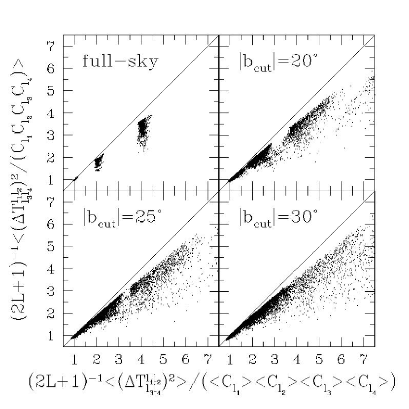
Figure 6.1: Variance of Normalized Trispectrum and Bare Trispectrum

Comparison of the variance of the normalized trispectrum with that of the bare trispectrum for $l_{1}\leq l_{2}<l_{3}\leq l_{4}$ and $L\neq 0$ (group (a)). These are derived from simulated realizations of a Gaussian sky. The top-left panel shows the case of full sky coverage, while the rest of panels show the cases of incomplete sky coverage. The top-right, bottom-left, and bottom-right panels use the $20^{\circ}$, $25^{\circ}$, and $30^{\circ}$ Galactic cuts, respectively.

6.3 Testing Gaussianity of the DMR Map

In this section, we test Gaussianity of the DMR data using the normalized trispectrum. Before performing the analysis, we should recall that even if CMB is exactly Gaussian, there are significant, non-zero unconnected trispectrum terms for $L=0$ or $l_{1}=l_{2}=l_{3}=l_{4}$. We should analyze these configurations separately from the others for which the unconnected terms vanish.

6.3.1 Classification of trispectrum configurations

We divide the measured 21,012 modes into four groups:

• $l_{2}\neq l_{3}$, and $L\neq 0$ (16,554 modes)

• $l_{2}=l_{3}$, $l_{1}\neq l_{4}$, and $L\neq 0$ (4,059 modes)

• $l_{1}=l_{2}=l_{3}=l_{4}$, and $L\neq 0$ (209 modes)

• $L=0$ (190 modes)

Note that all the groups satisfy $l_{1}\leq l_{2}\leq l_{3}\leq l_{4}$, $\max(l_{2}-l_{1},l_{4}-l_{3})\leq L\leq\min(l_{1}+l_{2},l_{3}+l_{4})$, $l_{1}+l_{2}+L=\mbox{even}$, and $l_{3}+l_{4}+L=\mbox{even}$.

The groups (a) and (b) are most sensitive to non-Gaussian signals, as for which the unconnected terms (Eq.(6.8)) vanish on the full sky. On the other hand, the groups (c) and (d) are dominated by the unconnected terms, and thus less sensitive to non-Gaussianity. These statements should, however, depend upon what kind of non-Gaussianity exists in the data. If non-Gaussian signals are subject to the groups (c) and (d) only, then the groups (a) and (b) become the least sensitive modes to the non-Gaussianity.

On the incomplete sky, the unconnected terms also contaminate the groups (a) and (b) through the mode-mode coupling. We take this effect into account by using the Monte-Carlo simulations that use the same Galactic cut as the data.

We discriminate between the group (a) and the group (b) in terms of the covariance matrix: the covariance matrix of the group (a) is diagonal, while that of the group (b) is not diagonal in $L$. We discriminate between the group (c) and the group (d) in terms of the statistical power: the group (d) has no statistical power of testing Gaussianity. The reason is as follows. For the group (d), the estimator given by equation (6.7) becomes $T^{l_{1}l_{1}}_{l_{3}l_{3}}(0)=(-1)^{l_{1}+l_{3}}\sqrt{(2l_{1}+1)(2l_{3}+1)}C_{l_{1}}C_{l_{3}}$. The normalized bispectrum for the group (d) is thus just a pure number,

$$\frac{T^{l_{1}l_{1}}_{l_{3}l_{3}}(0)}{C_{l_{1}}C_{l_{3}}}=(-1)^{l_{1}+l_{3}}\sqrt{(2l_{1}+1)(2l_{3}+1)}.$$ (6.13)

This property holds regardless of Gaussianity. Even strongly non-Gaussian fields give exactly the same number. It thus follows from this result that we cannot measure the connected trispectrum for $L=0$.

This is unfortunate. It is the connected part of $T^{l_{1}l_{1}}_{l_{3}l_{3}}(0)$ that contributes to the covariance matrix of the power spectrum,

$$\left<C_{l}C_{l^{\prime}}\right>-\left<C_{l}\right>\left<C_{l^{\prime}}\right>=\frac{2\left<C_{l}\right>^{2}}{2l+1}\delta_{ll^{\prime}}+\frac{(-1)^{l+l^{\prime}}}{\sqrt{(2l+1)(2l^{\prime}+1)}}\left<T^{ll}_{l^{\prime}l^{\prime}}(0)\right>_{\rm c},$$ (6.14)

where $\left<T^{ll}_{l^{\prime}l^{\prime}}(0)\right>_{\rm c}$ is the ensemble average of the connected $T^{ll}_{l^{\prime}l^{\prime}}(0)$. Even if we find the groups (a)–(c) consistent with Gaussianity, we can conclude nothing about the power spectrum covariance, unless we have a model for the connected trispectrum. We will discuss this point in § LABEL:sec:conclusion_obstl.

Henceforth, we analyze the groups (a)–(c) only, while we have used the group (d) to see if our code works properly. Our code reproduces equation (6.13) very well, and the numerical error is at most of order $10^{-4}$.

6.3.2 Gaussianity test

To quantify statistical significance of the measured trispectrum, we use a statistic $P$, which is the probability of the measured normalized trispectrum being greater than those drawn from the Monte–Carlo simulations:

$$P_{\alpha}\equiv\frac{N\left(\left|J_{\alpha}^{\rm DMR}\right|>\left|J_{\alpha}^{\rm MC}\right|\right)}{N_{\rm total}},$$ (6.15)

where $J_{\alpha}$ denotes the normalized trispectrum, $N_{\rm total}=30,000$ is the total number of the simulated realizations, and $\alpha$ represents a set of $(l_{1},l_{2},l_{3},l_{4},L)$. The distribution of $P_{\alpha}$ is uniform if the DMR map is consistent with Gaussian, for which there are equal number of modes in each bin of $P$. For example, when we calculate $P_{\alpha}$ for all 21,012 $\alpha$’s, we expect a Gaussian field to give 210.12 modes in $\Delta P=1\%$ bin. If we detect the normalized trispectrum significantly, then the number of modes having higher $P$ is much larger than the expectation value for a Gaussian field.

In chapter 5, we have proven the $P$ distribution uniform, if the DMR data are consistent with the simulated realizations (see Eq.(5.14)). We have also shown that this property holds regardless of the distribution function of $J_{\alpha}^{\rm MC}$.

We calculate the KS statistic for the $P$ distribution in comparison with the uniform distribution, to quantify how well the $P$ distribution is uniform. We calculate the KS statistic for the groups (a)–(c) separately. Table 6.1 summarizes the KS-test results, and figures 6.2–LABEL:fig:KS_norm_tl_unc2 plot the cumulative $P$ distribution, for which we have calculated the KS statistic. We find that the measured trispectrum is comfortably consistent with Gaussianity for all of the analyzed groups, (a)–(c).

Since the groups (a) and (b) are zero for Gaussian fields, these groups provide the strongest constraint on generic non-Gaussian fluctuations. As we have done in chapter 5 for the angular bispectrum, if we have predictions for the CMB angular trispectrum (e.g., appendix LABEL:app:CH), then our measurement tests those predictions.

Table 6.1: Gaussianity Test with Normalized Trispectrum

Probability of the measured trispectrum being consistent with Gaussianity (the rightmost column) for the three different Galactic cuts. The probability is derived from the KS test for the $P$ distribution in comparison with the uniform distribution. The group (a) comprises the modes of $l_{2}\neq l_{3}$, and $L\neq 0$ (16,554 modes), the group (b) of $l_{2}=l_{3}$, $l_{1}\neq l_{4}$, and $L\neq 0$ (4,059 modes), and the group (c) of $l_{1}=l_{2}=l_{3}=l_{4}$, and $L\neq 0$ (209 modes).

group	# of modes	Galactic cut	probability [%]
(a)	16,554	$20^{\circ}$	5.4
		$25^{\circ}$	12
		$30^{\circ}$	48
(b)	4,059	$20^{\circ}$	38
		$25^{\circ}$	2.5
		$30^{\circ}$	5.2
(c)	209	$20^{\circ}$	41
		$25^{\circ}$	71
		$30^{\circ}$	63

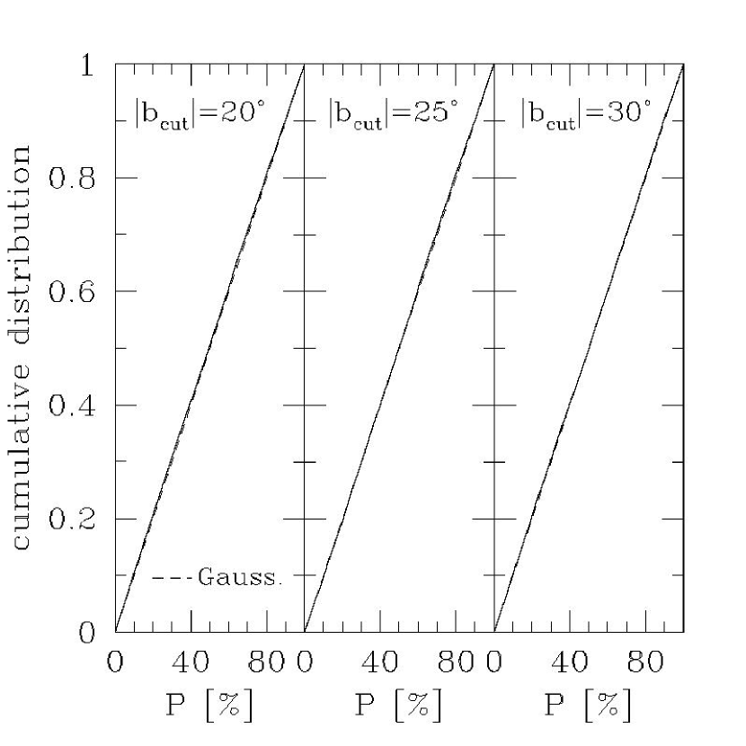
Figure 6.2: KS Test for Gaussianity with Trispectrum I

Cumulative $P$ Distribution (Eq.(6.15)), for which we calculate the KS statistic. $P$ is the probability of the normalized trispectrum, $T^{l_{1}l_{2}}_{l_{3}l_{4}}(L)/\left[(2L+1)C_{l_{1}}C_{l_{2}}C_{l_{3}}C_{l_{4}}\right]^{1/2}$, for the group (a) ($L\neq 0$ and $l_{1}\leq l_{2}<l_{3}\leq l_{4}$), measured on the COBE DMR $53+90~{}{\rm GHz}$ sky map, being larger than those drawn from the Monte–Carlo simulations. There are 16,654 modes. From left to right panels, we use the $20^{\circ}$, $25^{\circ}$, and $30^{\circ}$ Galactic cuts, respectively. The dashed lines show the expectation value for a Gaussian field. The KS statistic gives the probability of the distribution being consistent with Gaussianity as 5.4%, 12%, and 48% for the three Galactic cuts, respectively.

Figure 6.3: KS Test for Gaussianity with Trispectrum II

The same as figure 6.2 but for the group (b) ($l_{2}=l_{3}$, $l_{1}\neq l_{4}$, and $L\neq 0$). There are 4,059 modes. The KS statistic gives the probability of the distribution being consistent with Gaussianity as 38%, 2.5%, and 5.2% for the three Galactic cuts, respectively.