Problems and Progress in Astrophysical Dynamos

Abstract

Astrophysical objects with negligible resistivity are often threaded by large scale magnetic fields. The generation of these fields is somewhat mysterious, since a magnetic field in a perfectly conducting fluid cannot change the flux threading a fluid element, or the field topology. Classical dynamo theory evades this limit by assuming that magnetic reconnection is fast, even for vanishing resistivity, and that the large scale field can be generated by the action of kinetic helicity. Both these claims have been severely criticized, and the latter appears to conflict with strong theoretical arguments based on magnetic helicity conservation and a series of numerical simulations. Here we discuss recent efforts to explain fast magnetic reconnection through the topological effects of a weak stochastic magnetic field component. We also show how mean-field dynamo theory can be recast in a form which respects magnetic helicity conservation, and how this changes our understanding of astrophysical dynamos. Finally, we comment briefly on why an asymmetry between small scale magnetic and velocity fields is necessary for dynamo action, and how it can arise naturally.

1 Introduction

Magnetic fields have played a curious role in astrophysics, being both commonplace and poorly understood. They are ubiquitous in ionized systems, from the interiors of stars to the hot interstellar medium. The magnetic energy density is typically roughly comparable to the turbulent kinetic energy density. In stellar interiors, this means that magnetic fields tend to play a small role. In the interstellar medium, and in stellar coronae, their role is large, and consequently a matter of intense debate. In accretion disks the typical magnetic field energy density is probably an order of magnitude below the ambient gas pressure (e.g. hgb95 ; hgb96 ; shgb96 ; bnst95 ; bnst96 ) but they play a critical role in the outward transfer of angular momentum and the dissipation of orbital energy. Moreover, in optically thin environments the presence of a strong magnetic field can have a dramatic effect on the luminosity and spectrum of an object. A clear understanding of the generation and dynamics of magnetic fields is important to astrophysics in many ways. Unfortunately, their dynamics has not been well understood, at least judging by the diversity of opinions found in the literature cv91 ; p92 ; ka92 ; vpr93 ; bz95 . Consequently, arguments which cite magnetic fields as a dynamically important element in any particular object have tended to rely on phenomenology, rather than any sort of fundamental explanation.

Fortunately, over the last ten years, and especially quite recently, there has been significant progress in this area. First, although direct observations of high conductivity magnetic field dynamics are still restricted to the solar wind and the Sun, improvements in resolution have made it possible to watch magnetic fields evolve in real time khm98 , and to measure the power spectrum of magnetohydrodynamic (MHD) turbulence in the solar wind directly lsnm98 . Second, numerical simulations have reached the point where it is possible to simulate simple MHD systems with $\sim 10^{8}$ cells over many dynamical times. Third, a better understanding has been reached in terms of MHD turbulence theory (for a review see the chapter by Cho, Lazarian & Vishniac in this volume).

These results encourage us to believe that the many remaining problems are ripe for further progress. These problems range from the nature of dynamo processes in stars, accretion disks, and galaxies, to the question of how magnetic fields reconnect on dynamical time scales, with apparent disregard for the constraint due to flux-freezing. To be more precise, in the limit of negligible resistivity, the magnetic field in a fluid medium is frozen, the sense that neither the magnetic flux threading a fluid element, nor the field topology, can change. Magnetic reconnection, the exchange of partners between adjacent field lines violates the second condition, while the generation of a large scale field through dynamo action apparently violates the first.

Conventional mean field dynamo theory (see m78 ; p79 ; kr80 for reviews) allows a large-scale magnetic field to grow exponentially from a seed field (see r88 ; l92 ) at the expense of small-scale turbulent energy through a process of spiral twisting and reconnection, illustrated in Fig. 1.

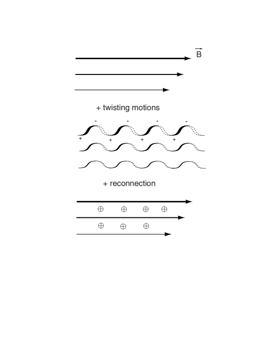
Figure 1: The mean-field dynamo in action. Anisotropic turbulence twists the field lines into spirals. Reconnection restores the original field lines, but a vertical gradient in the strength of the spirals generates a net flux out of the page.

This process starts with a set of large scale parallel field lines pointing in some arbitrary direction. If the underlying turbulence has a tendency to twist the field lines into spirals with a preferred handedness (i.e. the velocity field has some net helicity), then reconnection on two dimensional surfaces between adjacent spirals will produce a new field, at right angles to the old one, provided that there is a systematic gradient in the strength of the spirals. The new field component is at right angles to both the gradient and the old field component. In a differentially rotating system, we can get a dynamo if the original field direction is in the $\hat{\phi}$ direction, and the dynamo process produces a radial field component. Differential shearing of $B_{r}$ will then drive the azimuthal field component, closing the cycle. This is the ‘$\alpha-\Omega$ dynamo’. In the absence of global shear, we need a second round of dynamo action, which gives an $\alpha^{2}$ dynamo. This process can be given a systematic mathematical treatment by a suitable choice of averaging procedures.

There are two ways in which this picture ignores, rather than solves, the difficulties imposed by flux-freezing. The more obvious point is that adjacent spiral field lines are assumed to reconnect quickly. Without this assumption the field will accumulate small scale tangled knots which will quickly suppress dynamo action, and the large scale magnetic field will saturate far below equipartition with the surrounding turbulence. Unfortunately, if reconnection happens at the rate allowed by the generally accepted Sweet-Parker model p57 ; s58 , it is far too slow. However, there are observations which suggest that this represents more of a challenge for theorists than a real constraint on the evolution of magnetic fields. If reconnection is slow, turbulence would cause many magnetic reversals per parsec within the interstellar medium. Observations, on the contrary, show that magnetic field is coherent over the scales of hundreds of parsecs. This fact, as well as direct observations of large and small scale Solar flares d95 , suggest that the rate of reconnection is many orders of magnitude more rapid than allowed by the Sweet-Parker model. As this example shows, the importance of reconnection in astrophysics is not limited to understanding the dynamo process. The process of reconnection is an integral part of the transfer of magnetic energy to fluid and particle motion in stellar coronae and in the interstellar medium. More generally, it is impossible to claim that we understand MHD unless we can predict whether crossing magnetic flux tubes will reconnect or bounce from one another.

A more subtle difficulty arises from the process by which straight field lines are twisted into spirals. This is intuitively appealing if we consider field lines as isolated strings of infinitesimal radius. More realistically, the field occupies a non-zero volume. Twisting a tube into a spiral shape requires that we either allow the ends to slip, or allow parts of the tube to twist in the opposite sense. There is a geometrical constraint which is ignored in the standard picture. This objection can be given a rigorous mathematical form, the conservation of magnetic helicity, which we will describe in §3.

How do numerical simulations of dynamo activity compare to mean-field dynamo theory? Computer simulations of dynamos can be divided into two classes. There are simulations in which some local instability (convection, the Balbus-Hawley instability etc.) is allowed to operate, and there are simulations in which the turbulence is driven externally, usually in such a way as to guarantee the presence of a net fluid helicity. The former simulations are often successful at generating large scale magnetic fields whose energy density is at least as great as the turbulent energy density (e.g.bnst95 ; hb92 ; gr95 ). The latter are less successful, in the sense that the energy density of the large scale magnetic field is often quite modest (e.g. m81 ; b00 ). In particular there are simulations (ch96 ; b01 ) which produce dynamos in a computational box, with forced heliacal turbulence. These dynamos show a steep inverse correlation between the dynamo growth rate and the conductivity. Naively extrapolating to astrophysical regimes suggests that magnetic dynamos driven by fluid helicity would take enormous amounts of time to grow. This conclusion is sharply at odds with evidence for rapid and efficient stellar dynamos.

Here we discuss recent work on the problems of fast reconnection and magnetic helicity conservation in astrophysical dynamos. For reconnection we concentrate on a generic reconnection scheme that appeals to magnetic field stochasticity as the critical property that accelerates reconnection (lv99 , see lv00 for a review). Collisionless plasma effects which may also accelerate magnetic reconnection are addressed in the chapter by Bhattacharjee in this volume. We will typically assume that the evolution of the magnetic field is described by the simplest form of the induction equation

$$\partial_{t}{\bf B}={\bf\nabla\times v\times B}+\eta\nabla^{2}{\bf B},$$ (1)

although we will make reference to work which includes more realistic treatments of collisionless plasma effects.

2 Rates of Magnetic Reconnection

A simple dimensionless measure of the importance of resistivity, $\eta$, in a conducting fluid is the Lundquist number $\equiv V_{A}L/\eta$, where $V_{A}\equiv B/(4\pi\rho)^{1/2}$ is the Alfvén velocity and $L$ is a typical scale of the system. When fluid velocities are of order the Alfvén speed, as is usual in astrophysics, this is a crude estimate of the ratio of the first and second terms in equation (1). Typically this number is very large under most astrophysical circumstances, and flux freezing should be a good approximation. More precisely, the coefficient of magnetic field diffusivity in a fully ionized plasma is $\eta=c^{2}/(4\pi\sigma)=10^{13}T^{-3/2}$ cm² s^-1, where $\sigma=10^{7}T^{3/2}$ s^-1 is the plasma conductivity and $T$ is electron temperature. The characteristic time for field diffusion through a plasma slab of size $L$ is $L^{2}/\eta$, which is large for any “astrophysical” $L$.

What happens when magnetic field lines intersect? Do they deform each other and bounce back or they do change their topology? This is the central question of the theory of magnetic reconnection. In fact, the whole dynamics of magnetized fluids and the back-reaction of the magnetic field depends on the answer.

2.1 The Sweet-Parker Scheme and its Modifications

The literature on magnetic reconnection is rich and vast (see, for example, pf00 and references therein). We start by discussing a robust scheme proposed by Sweet and Parker p57 ; s58 . In this scheme oppositely directed magnetic fields are brought into contact over a region of length $L_{x}$ (see Fig. 2). In general there will be a shared component, of the same order as the reversed component. However, this has only a minor effect on our discussion. The gradient in the magnetic field is confined to the current sheet, a region of vertical size $\Delta$, within which the magnetic field evolves resistively. The velocity of reconnection, $V_{r}$, is the speed with which magnetic field lines enter the current sheet, and is roughly $\eta\approx V_{r}\Delta$. Arbitrarily high values of $V_{r}$ can be achieved (transiently) by decreasing $\Delta$. However, for sustained reconnection there is an additional constraint imposed by mass conservation. The plasma initially entrained on the magnetic field lines must escape from the reconnection zone. In the Sweet-Parker scheme this means a bulk outflow, parallel to the field lines, within the current sheet. Since the mass enters along a zone of width $L_{x}$, and is ejected within a zone of width $\Delta$, this implies

$$\rho V_{rec}L_{x}=\rho^{\prime}V_{A}\Delta~{}~{}~{},$$ (2)

where we have assumed that the outflow occurs at the Alfvén velocity. This is actually an upper limit set by energy conservation. If we ignore the effects of compressibility $\rho=\rho^{\prime}$ and the resulting reconnection velocity allowed by Ohmic diffusivity and the mass constraint is

$$V_{rec,sweet-parker}\approx V_{A}{\cal R}_{L}^{-1/2},$$ (3)

where ${\cal R}_{L}$ is the Lundquist number using the current sheet length. Depending on the specific astrophysical context, this gives a reconnection speed which lies somewhere between $10^{-3}$ (stars) and $10^{-10}$ (the galaxy) times $V_{A}$.

Figure 2: Upper plot: Sweet-Parker scheme of reconnection. Middle plot: illustration of stochastic reconnection that accounts for field line noise. Lower plot: a close-up of the contact region. Thick arrows depict outflows of plasma. From lv00 .

It is well known that using the Sweet-Parker reconnection rate it is impossible to explain solar flares. For the reasons given in the introduction, it is also well known that it is impossible to reconcile dynamo theory with observations without some substantially faster reconnection scheme. Consequently, for forty years discussions of reconnection speeds have tended to focus on mechanisms that might give reconnection speeds close to $V_{A}$, i.e. ‘fast’ reconnection. In general, we can divide schemes for fast reconnection into those which alter the microscopic resistivity, broadening the current sheet, and those which change the global geometry, thereby reducing $L_{x}$. Ultimately, a successful scheme should satisfy basic physical constraints without requiring contrived geometries or boundary conditions. In the near term, we can gain some insight into the likely nature of the solution by considering that reconnection is not always fast. Magnetic field lines in the solar corona and chromosphere which could reach a lower energy configuration through reconnection do not always immediately do so. Furthermore, a solution which relies entirely on collisionless effects, for example, would imply that field lines do not reconnect in dense environments, which would leave a major problem in understanding the nature of stellar dynamos.

Attempts to accelerate Sweet-Parker reconnection are numerous. We start by considering schemes to broaden the current sheet. Anomalous resistivity is known to broaden current sheets in laboratory plasmas. It is present in the reconnection layer when the field gradient is so sharp that the electron drift velocity is of the order of thermal velocity of ions $u=(kT/m)^{1/2}$p79 . In other words, when $j>j_{cr}=Neu$. If the current sheet has a width $\delta$ with a change in the magnetic field $\Delta B$ then $4\pi j=c\Delta B/\delta$. The effective resistivity increases nonlinearly as $j$ becomes greater than $j_{cr}$, thereby broadening the current sheet. We can find an upper limit to this effect by assuming that $j$ never gets very much larger than $j_{cr}$, that is $\delta\approx\frac{c\Delta B}{4\pi Neu}$. Expressing $\delta$ in terms of the ion cyclotron radius $r_{c}=(muc)/(eB_{tot})$, where $B_{tot}$ is the total magnetic field (including any shared component) we find

$$\delta\approx r_{c}\left(\frac{V_{A}}{u}\right)^{2}\frac{\Delta B}{B_{tot}}~{}~{}~{},$$ (4)

which agrees with p79 up to the factor $\Delta B/B_{tot}$, which equals 1 in that treatment. Combining (2) and (4) one gets lv99

$$V_{rec,anomalous}\approx V_{A}\frac{r_{c}}{L_{x}}\left(\frac{V_{A}}{u}\right)^{2}\frac{\Delta B}{B_{tot}}~{}~{}~{}.$$ (5)

Equation (5) shows that the enhanced reconnection velocity is still much less than the Alfven velocity if $L_{x}$ is much greater than the ion Larmor (cyclotron) radius. In general, “anomalous reconnection” is important when the thickness of the reconnection layer in the Sweet-Parker reconnection scheme is less than $\delta$. However, for typical interstellar magnetic fields the Larmor radius $r_{c}$ is $\sim 10^{7}$ cm and anomalous effects are negligible.

Tearing modes are a robust instability connected to the appearance of narrow current sheets fkr63 . The resulting turbulence will broaden the reconnection layer and enhance the reconnection speed. Here we give an estimate of this effect and show that while it represents a significant enhancement of Sweet-Parker reconnection of laminar fields, it leaves reconnection slow. One difficulty with many earlier studies of reconnection in the presence the tearing modes stemmed from the idealized two dimensional geometry assumed for reconnection. In two dimensions tearing modes evolve via a stagnating non-linear stage related to the formation of magnetic islands. This leads to a turbulent reconnection zone ml85 , but the current sheet remains narrow and its effects on the overall reconnection speed are unclear. This nonlinear stagnation stage does not emerge when realistic three dimensional configurations are considered lv99 . In any realistic circumstances field lines are not exactly antiparallel. Consequently, we expect that instead of islands one finds nonlinear Alfvén waves in three dimensional reconnection layers. The tearing instability proceeds with growth rates determined by the linear growth phase while the resulting magnetic structures propagate out of the reconnection region at the Alfvén speed.

The dominant mode will be the longest wavelength mode, whose growth rate will be

$$\gamma\approx{\eta\over\Delta^{2}}\left({V_{A}\lambda_{\|}\over\eta}\right)^{2/5}.$$ (6)

The transverse spreading of the plasma in the reconnection layer will start to stabilize this mode when its growth rate is comparable to the transverse shear $V_{A}/\lambda_{\|}$ bss79 . At this point we have $V_{rec,local}\approx\gamma\Delta$ and lv99

$$V_{rec,tearing}=V_{A}\left({\eta\over V_{A}L_{x}}\right)^{3/10},$$ (7)

which is substantially faster than the Sweet-Parker rate, but still very slow in any astrophysical context. Note that unlike anomalous effects, tearing modes do not require any special conditions and therefore should constitute a generic scheme of reconnection.

Finally, we note that there is a longstanding, but controversial suggestion, that ions tend to scatter about once per cyclotron period, ‘Bohm diffusion’ b49 . Even if this is correct, the effective diffusivity of magnetic field lines would still be only $\eta_{\rm Bohm}\sim V_{A}r_{c}$. While this would be a large increase over Ohmic resistivity, it produces fast reconnection, of order $V_{A}$, only if $r_{c}\sim L_{x}$. It therefore fails as an explanation for fast reconnection for the same reason that anomalous resistivity does.

2.2 X-point Reconnection

The failure to find fast reconnection speeds through current sheet broadening has stimulated interest in fast reconnection through radically different global geometries. Petschek p64 conjectured that reconnecting magnetic fields would tend to form structures whose typical size in all directions is determined by the resistivity (‘X-point’ reconnection). This results in a reconnection speed of order $V_{A}/\ln{\cal R}_{L}$. However, attempts to produce such structures in numerical simulations of reconnection have been disappointing. Typically the X-point region collapses towards the Sweet-Parker geometry as the Lundquist number becomes large b84 ; b86 ; b96 ; wmb96 ; wb96 . One way to understand this collapse is to consider perturbations of the original X-point geometry. In order to maintain this geometry shocks are required in the original (Petschek) version of this model. These shocks are, in turn, supported by the flows driven by fast reconnection, and fade if $L_{x}$ increases. Naturally, the dynamical range for which the existence of such shocks is possible depends on the Lundquist number and shrinks when fluid conductivity increases. The apparent conclusion is that, at least in the collisional regime, reconnection occurs through narrow current sheets.

One may invoke collisionless plasma effects to stabilize the X-point reconnection (for collisionless plasma). For instance, a number of authors sddb98 ; sd98 ; sdrd99 have reported that in a two fluid treatment of magnetic reconnection, a standing whistler mode can stabilize an X-point with a scale comparable to the ion plasma skin depth, $c/\omega_{pi}\sim(V_{A}/c_{s})r_{L}$. The resulting reconnection speed is a large fraction of $V_{A}$, and apparently independent of $L_{x}$, which would suggest that something like Petschek reconnection emerges in the collisionless regime. This possibility is discussed at length in the chapter by Bhattacharjee (this volume). However, these studies have not yet demonstrated the possibility of fast reconnection for generic field geometries, since they assume that there are no bulk forces acting to produce a large scale current sheet. Similarly, those studies do not account for fluid turbulence. Magnetic fields embedded in a turbulent fluid will give fluctuating boundary conditions for the current sheets. On the other hand, boundary conditions need to be fine tuned for a Petschek reconnection scheme pf00 .

Finally, we note that a number of researchers have claimed that turbulence may accelerate reconnection (for example, s88 , where tearing modes are used as the source of the turbulence). The general idea is that turbulent motions can provide an effect transport coefficient $\sim\langle v^{2}\rangle\tau$ p79 . However, a closer examination of this process has convincingly demonstrated that an unrealistic amount of energy is required to mix field lines unless they are almost exactly anti-parallel p92 . In the next section we will discuss a mechanism that, when it works, should produce reconnection under a broad range of field geometries, without regard to the particle collision rate.

2.3 Stochastic Reconnection

Two idealizations were used in the preceding discussion. First, we considered reconnection in only two dimensions. Second, we assumed that the magnetized plasma has laminar field lines. The Sweet-Parker scheme can easily be extended into three dimensions, in the sense that one can take a cross-section of the reconnection region such that the shared component of the two magnetic fields is perpendicular to the cross-section. In terms of the mathematics nothing changes, but the outflow velocity becomes a fraction of the total $V_{A}$ and the shared component of the magnetic field will have to be ejected together with the plasma. This result has motivated researchers to do most of their calculations in 2D, which has obvious advantages for both analytical and numerical investigations.

However, physics in two and three dimensions are very different. This is true, for example, in hydrodynamic turbulence, partly because lines of vorticity have different dynamics when they are free to move around one another. Similarly, the ability of magnetic field lines to move past one another in three dimensions dramtically alters the topolical constraints on their dynamics. In lv99 we considered three dimensional reconnection in a turbulent magnetized fluid and showed that reconnection is fast. This result cannot be obtained by considering two dimensional turbulent reconnection (cf. ml85 ). This point has been the source of significant confusion. Turbulent reconnection has usually been used to refer to reconnection driven by the turbulent transport of magnetic flux, as discussed in the previous subsection. In other words, one looks for a net flux transport term, operating on microscales, that is proportional to magnetic field gradients and has a coefficient which is independent of the resistivity. This process was recently examined, and severely criticized, in kd01 , under the mistaken impression that it the critical physical process in stochastic reconnection. Instead, stochastic reconnection is a geometric effect arising from the appearance of stochastic field line wandering in three dimensions, which gives rise to a broad outflow from the current sheet, but has little effect on the current sheet structure. Below we briefly discuss the idea of stochastic reconnection, while the full treatment of the problem is given in lv99 .

MHD turbulence guarantees the presence of a stochastic field component, although its amplitude and structure clearly depends on the amplitude and the turbulence driving mechanism. Our model of the field line stochasticity also depends on our ability to model generic MHD turbulence. We consider the case in which there exists a large scale, well-ordered magnetic field, of the kind that is normally used as a starting point for discussions of reconnection. This field may, or may not, be ordered on the largest conceivable scales. However, we will consider scales smaller than the typical radius of curvature of the magnetic field lines, or alternatively, scales below the peak in the power spectrum of the magnetic field, so that the direction of the unperturbed magnetic field is a reasonably well defined concept. In addition, we expect that the field has some small scale ‘wandering’ of the field lines. On any given scale the typical angle by which field lines differ from their neighbors is $\phi\ll 1$, and this angle persists for a distance along the field lines $\lambda_{\|}$ with a correlation distance $\lambda_{\perp}$ across field lines (see Fig. 2).

The modification of the mass conservation constraint in the presence of a stochastic magnetic field component is self-evident. Instead of being squeezed from a layer whose width is determined by Ohmic diffusion, the plasma may diffuse through a much broader layer, $L_{y}\sim\langle y^{2}\rangle^{1/2}$ determined by the diffusion of magnetic field lines. (Here ‘$y$’ is the axis perpendicular to the mean field direction. See Fig. 2.) This suggests an upper limit on the reconnection speed of $\sim V_{A}(\langle y^{2}\rangle^{1/2}/L_{x})$. This will be the actual speed of reconnection if the progress of reconnection in the current sheet itself does not impose a smaller limit. The value of $\langle y^{2}\rangle^{1/2}$ can be determined once a particular model of turbulence is adopted, but it is obvious from the very beginning that this value is determined by field wandering rather than Ohmic diffusion, as in the Sweet-Parker model.

What about limits on the speed of reconnection that arise from considering the structure of the current sheet? In the presence of a stochastic field component, magnetic reconnection dissipates field lines not over their entire length $\sim L_{x}$ but only over a scale $\lambda_{\|}\ll L_{x}$ (see Fig. 2), which is the scale over which magnetic field line deviates from its original direction by the thickness of the Ohmic diffusion layer $\lambda_{\perp}^{-1}\approx\eta/V_{rec,local}$. If the angle $\phi$ of field deviation did not depend on the scale, the local reconnection velocity would be $\sim V_{A}\phi$, independent of resistivity. However, for any realistic model of MHD turbulence, $\phi$ ($=\lambda_{\perp}/\lambda_{\|}$, does depend on scale. Consequently, the local reconnection speed $V_{rec,local}$ is given by the usual Sweet-Parker formula but with $\lambda_{\|}$ instead of $L_{x}$, i.e. $V_{rec,local}\approx V_{A}(V_{A}\lambda_{\|}/\eta)^{-1/2}$. Also, it is apparent from Fig. 2 that $\sim L_{x}/\lambda_{\|}$ magnetic field lines will undergo reconnection simultaneously (compared to a one by one line reconnection process for the Sweet-Parker scheme). Therefore the overall reconnection rate may be as large as $V_{rec,global}\approx V_{A}(L_{x}/\lambda_{\|})(V_{A}\lambda_{\|}/\eta)^{-1/2}$. Whether or not this limit is important depends on the value of $\lambda_{\|}$.

The relevant values of $\lambda_{\|}$ and $\langle y^{2}\rangle^{1/2}$ depend on the magnetic field statistics. This calculation was performed in lv99 using the Goldreich-Sridhar model gs95 of MHD turbulence, the Kraichnan model (i63 ; k65 ) and for MHD turbulence with an arbitrary spectrum (limited only some basic physical constraints and which is in rough agreement with observations a95 ; lp00 ; sl02 ). In all the cases the upper limit on $V_{rec,global}$ was greater than $V_{A}$, so that the diffusive wandering of field lines imposed the relevant limit on reconnection speeds. Among these, the Goldreich-Sridhar model provides the best fit to observations (e.g. a95 ; sl02 ) and simulations cva ; cvb . In this case the reconnection speed was

$$V_{rec,up}=V_{A}\min\left[\left({L_{x}\over l}\right)^{\frac{1}{2}},\left({l\over L_{x}}\right)^{\frac{1}{2}}\right]\left({v_{l}\over V_{A}}\right)^{2},$$ (8)

where $l$ and $v_{l}$ are the energy injection scale and turbulent velocity at this scale respectively. We stress that the use of MHD turbulence models here is solely for the purpose of providing a well-defined model of field line stochasticity. The dynamics of the turbulent cascade are largely irrelevant and any process which leads to small scale field line stochasticity (e.g. footpoint motions for solar field lines) is a possible cause of fast reconnection.

In lv99 we also considered other processes that can impede reconnection and find that they are less restrictive. For instance, the tangle of reconnection field lines crossing the current sheet will need to reconnect repeatedly before individual flux elements can leave the current sheet behind. The rate at which this occurs can be estimated by assuming that it constitutes the real bottleneck in reconnection events, and then analyzing each flux element reconnection as part of a self-similar system of such events. This turns out to limit reconnection to speeds less than $V_{A}$, which is obviously true regardless. As the result equation (8) is not only an upper limit on the reconnection speed, but is the best estimate of its value.

Naturally, when turbulence is negligible, i.e. $v_{l}\rightarrow 0$, the field line wandering is limited to the Sweet-Parker current sheet and the Sweet-Parker reconnection scheme takes over. However, in practice this requires an artificially low level of turbulence that should not be expected in realistic astrophysical environments. Moreover, the release of energy due to reconnection, at any speed, will contribute to the turbulent cascade of energy and help drive the reconnection speed upward. This may be relevant to the slow onset, and rapid acceleration, of the reconnection process in solar flares.

We stress that the enhanced reconnection efficiency in turbulent fluids is only present if 3D reconnection is considered. In this case ohmic diffusivity fails to constrain the reconnection process as many field lines simultaneously enter the reconnection region. The number of lines that can do this increases with the decrease of resistivity and this increase overcomes the slow rates of reconnection of individual field lines. It is impossible to achieve a similar enhancement in 2D (see z98 ) since field lines can not cross each other.

There is a limited analogy one can draw between the enhancement of reconnection speeds in X-point models and increased rate of reconnection due to field line stochasticity. In both cases one gets a boost from a reduced parallel length scale. In the case of X-point models this effect is, usually by design, enormous since $L_{x}\rightarrow\Delta$. Stochastic reconnection depends on a relatively modest enhancement, since $L_{x}\rightarrow\lambda_{\|}(\Delta)\gg\Delta$. The bulk of the effect comes from the simultaneous reconnection of many independent flux elements, and the steady diffusion of the ejected plasma away from the current sheet. The main problem with X-point reconnection models, their tendency to collapse to narrow current sheets, is absent in stochastic reconnection, since in the latter case the current sheets stay narrow, and the diverging field lines are separated by other field lines, rather than by unmagnetized plasma.

A more subtle difficulty arises from our prescription for the structure of the stochastic field near the current sheet. We have assumed that we can apply the statistically homogeneous prescription for field line perturbations in a turbulent medium near planes where there is a dramatic change in the structure of the large scale magnetic field. This is not obvious. It may be that the presence of a strong shear in the field acts as a kind of internal surface, producing an altered, and perhaps greatly reduced, level of stochasticity. This kind of internal ‘shadowing’ does not appear in current simulations, but there has been little attempt to look for it, and the issue can only be resolved when detailed numerical simulations of stochastic reconnection are performed. Similarly, one may wonder if the systematic ejection of plasma along the field lines might modify their topological connections. In this case it seems more plausible to suppose that this would lead to an increase in the diffusion rate, rather than a decrease, but again no simulations of this process are available.

2.4 Reconnection in Partially Ionized Gas

A substantial fraction of the ISM in our galaxy is partially ionized, as well as photospheres of most stars. This motivates studies of the effect of neutrals on reconnection and MHD turbulence. The role of ion-neutral collisions is not trivial. On one hand, neutral particles tend to have a substantially longer mean free path, so that drag between the neutrals and ions may truncate the turbulent cascade at a relatively large scale. On the other hand, the ability of neutrals to diffuse perpendicular to magnetic field lines enhances reconnection rates, at least in the Sweet-Parker model.

Reconnection in partially ionized gases has been studied by various authors (nma92 ; zb97 ; vl99 ) in the context of the Sweet-Parker reconnection model. Our comments here are based on vl99 where we studied the diffusion of neutrals away from the reconnection zone. In general, in a partially ionized gas the reconnection zone consists of two distinct regions. A broad region, which width is determined by the ambipolar diffusivity, $\eta_{ambi}\approx V_{A}^{2}/t_{ni}$ where $t_{ni}$ is the neutral-ion collision rate, and a narrow region whose width is determined by the Ohmic diffusivity. Magnetic reconnection takes place in the narrow region, while the broader region allows a more efficient ejection of matter.

If the recombination time is short, then ions and neutrals are largely interchangeable and the reconnection speed is vl99

$$V_{rec}\approx V_{A}\left({V_{A}t_{in}\over L_{x}}\right)^{1/2}.$$ (9)

This is faster than the Sweet-Parker rate, but not fast in the sense of allowing reconnection speeds close to $V_{A}$. In practice, even this rate is typically unachievable. Under typical interstellar conditions the reconnection speed is limited by the recombination rate. That is, the rate at which ions recombine and leave the resistive region determines the speed of the whole process. Consequently, the ambipolar reconnection rates obtained in vl99 are insufficient either for fast dynamo models or for the ejection of magnetic flux prior to star formation. In fact, the increase in the reconnection speed stems entirely from the compression of ions in the current sheet, with the consequent enhancement of both recombination and ohmic dissipation. This effect is small unless the reconnecting magnetic field lines are almost exactly anti-parallel. As above, we expect that including the effects of anomalous resistivity and tearing modes may enhance reconnection speeds appreciably, but not to the extent of producing fast reconnection.

None of this work included the effects of field line stochasticity, which is critical for producing fast reconnection in ionized plasmas. We expect that in this case also the presence of turbulence will lead to substantially higher reconnection speeds. However, whether or not this produces fast reconnection must depend on the nature of the turbulent cascade in a partially ionized gas. Recent work, which is discussed in detail in the chapter by Cho, Lazarian & Vishniac in this volume, show that the magnetic field in a partially ionized gas has a much more complex structure than it is usually assumed. In fact, in clv02 we reported a new regime of MHD turbulence which is characterized by the existence of intermittent magnetic structures below the viscous cutoff scale. The root mean square perturbed magnetic field strength in these structures does not drop at smaller scales. However, the curvature scale (and therefore the divergence rate) for these structures does not decrease significantly as their perpendicular scale decreases. At sufficiently small scales the ions and neutrals will decouple, and a turbulent cascade, extending down close to resistive scales but involving only ions will appear.

The existence of strong magnetic field structures on small scales, and the reappearance of a strong turbulent cascade at very small scales, should lead to fast reconnection speeds through stochastic reconnection. However, it remains to be seen whether or not the intermediate scales, characterized by weak divergence of field lines, will impose a significant bottleneck on the reconnection plasma outflow. If it does, then the implication is that interstellar clouds with small ionized fractions may not allow fast reconnection. This conclusion would not pose any problems with galactic dynamo, but may be extremely important for other essential processes, e.g. star formation. This issue is examined further in lvc02 .

3 The Dynamo Process

3.1 Conventional Theory and its Problems

We start this section by briefly reviewing the standard approach to dynamo theory, and discussing various objections to it. Some of these objections center around the speed of reconnection, and can be safely ignored if reconnection is fast in a turbulent environment. In fact, since stochastic reconnection depends on small scale structure in the magnetic field, the claim that small scale structure tends to accumulate energy faster than the large scale field ka92 can be seen as self-limiting. A disproportionate growth in power on small scales will only continue until the reconnection speed is boosted to large fraction of $V_{A}$. However, as we have already mentioned, some objections to dynamo theory are more subtle and require substantial modification to mean-field dynamo theory.

The usual approach to the dynamo problem is to take equation (1), set $\eta=0$, and divide the velocity field into small scale turbulence and some large scale rotational motion. In order to follow the evolution of the large scale magnetic field, we write

$${\bf B}\equiv\langle{\bf B}\rangle+{\bf b}.$$ (10)

The brackets here denote averaging over scales somewhat larger than the turbulent eddy size. In other words, they indicate a smoothing process which averages out all small scale features. The field $\langle{\bf B}\rangle$ is the ‘mean field’. The dynamo process can be written in mathematical terms by approximating the evolution of the small scale field component, ${\bf b}$, as

$$\partial_{t}{\bf b}\approx{\bf\nabla\times v\times}\langle{\bf B}\rangle,$$ (11)

and substituting the result into the evolution equation for the large scale field,

$$\partial_{t}\langle{\bf B}\rangle={\bf\nabla\times}\langle{\bf v\times b}\rangle.$$ (12)

In a turbulent, incompressible and homogeneous plasma this implies

$$\partial_{t}\langle{\bf B}\rangle={\bf\nabla\times}({\bf\alpha\cdot B})+{\bf\nabla\cdot}({\bf D_{T}\cdot\nabla})\langle{\bf B}\rangle.$$ (13)

Here $\alpha$, the kinetic helicity, and ${\bf D_{T}}$, the turbulent diffusion tensor, are dyads given by

$$\alpha_{il}\equiv\epsilon_{ijk}\langle v_{j}\partial_{l}v_{k}\rangle\tau_{c},$$ (14)

and

$$D_{T,ij}\equiv\langle v_{i}v_{j}\rangle\tau_{c},$$ (15)

where $\tau_{c}$ is the eddy correlation time. The component of the electromotive force along the large scale field direction, $\langle{\bf\hat{B}}\rangle\cdot\langle{\bf v\times b}\rangle$, is the piece that can drive an increase in the large scale magnetic field. (The component perpendicular to $\langle{\bf B}\rangle$ gives an effective large scale field velocity, that is, it affects the transport of the field rather than its generation.) The trace of $\alpha$ divided by $\tau_{c}$ is what is usually referred to as the kinetic helicity, and it is often assumed for convenience that ${\bf\alpha}$ is a scalar times the identity matrix. In symmetric turbulence $\alpha$ vanishes, but ${\bf D_{T}}$ does not. In fact, since a successful dynamo requires non-vanishing diagonal components for $\alpha$, we can see from this expression that a successful dynamo should require symmetry breaking along all three principal axes.

The appearance of $D_{T}$ in equation (13) would seem to vindicate the use of turbulent diffusion in astrophysical MHD. There are two reasons why this is not quite right. First, fast reconnection is implicit in this kind of averaging argument. Rather than appealing to turbulent diffusion as an explanation for fast reconnection, we are actually using our understanding of fast reconnection to explain diffusion. The second point is less formal and more important. Equation (13) is not a realistic description of the evolution of $\langle{\bf B}\rangle$. As noted in §1, twisting magnetic field lines into spirals is not easily accomplished, and numerical simulations do not support the use of equation (13).

3.2 Magnetic Helicity Conservation Constraint

The fundamental problem is that there is an important mathematical constraint that follows from equation (1), which is not respected by equation (13). The magnetic helicity, defined as $H\equiv{\bf A}\cdot{\bf B}$ evolves according to

$$\partial_{t}H=-{\bf\nabla\cdot}\left[{\bf A\times}({\bf v\times B}+{\bf\nabla\Phi})\right]-\eta{\bf B\cdot\nabla\times B},$$ (16)

where $\Phi$ is an arbitrary function of space and time. For the Coulomb gauge, which turns out to be a convenient choice, we require

$$\nabla^{2}\Phi={\bf\nabla\cdot}({\bf v\times B}).$$ (17)

In the limit of vanishing resistivity, this not only implies that the volume integrated magnetic helicity vanishes, it also implies that the magnetic helicity of any individual flux tube is separately conserved t74 .

For a non-zero, but very small, $\eta$, we can transfer magnetic helicity from one flux tube to another. However, since $H$ is of order $LB^{2}$, where $L$ is a characteristic scale of the field, it takes less energy to hold magnetic helicity on large scales than on eddy scales, and a divergent amount on infinitesimal scales. Consequently, in the limit of vanishing resistivity the resistive term in equation (16) does not affect the global conservation of helicity, even in the presence of fast reconnection, as long as reconnection only occurs in an infinitesimal fraction of the plasma volume. On the other hand, the conservation of magnetic helicity for individual flux tubes is completely lost. The implication is that global magnetic helicity conservation is a good approximation for laboratory plasmas, a point that was originally stressed by Taylor t74 , and an even better one for astrophysical systems.

How does this affect dynamo theory? The large scale distribution of magnetic helicity can be divided into a piece carried by large scale magnetic structures and a piece carried by small scale structures, or

$$\langle H\rangle=\langle{\bf A}\rangle\cdot\langle{\bf B}\rangle+\langle{\bf a}\cdot{\bf b}\rangle.$$ (18)

Henceforth we will use $h\equiv\langle{\bf a}\cdot{\bf b}\rangle$. The evolution of the first piece, in a perfectly conducting fluid, is

$$\partial_{t}(\langle{\bf A}\rangle\cdot\langle{\bf B}\rangle)=2\langle{\bf B}\rangle\cdot\langle{\bf v\times b}\rangle-{\bf\nabla\cdot}\left[\langle{\bf A}\rangle{\bf\times}(\langle{\bf v\times b}\rangle+{\bf\nabla}\langle\Phi\rangle)\right].$$ (19)

The second term on the right hand side is the magnetic helicity transport driven by mean-field terms. The first represents the exchange of magnetic helicity between large and small scales. This term is proportional to the component of the electromotive force which drives the dynamo process. In other words, the generation of a large scale magnetic field is a direct consequence of the transfer of magnetic helicity between large and small scales.

The point that MHD turbulence transfers magnetic helicity to the largest available scales, even if that scale is much larger than any eddy scale, is well known f75 ; smg94 ; smo95 . We can estimate the rate at which $h$ is transferred to large scale magnetic field structures by considering its role in biasing the value of the electromotive force vc01 . The inverse cascade rate is

$$\tau_{cascade}^{-1}\sim{V_{A}^{2}\over\langle v^{2}\rangle}\tau_{c}^{-1}.$$ (20)

For a large scale magnetic field in equipartition with the turbulent cascade this implies that magnetic helicity is transferred to the large scale field in one eddy turn over time. This suggests that unless the large scale field is very weak it is reasonable to take

$$H\approx\langle{\bf A}\rangle\cdot\langle{\bf B}\rangle.$$ (21)

Then combining equations (19) and (21) we see that

$$2\langle{\bf B}\rangle{\bf\cdot}\langle{\bf v\times b}\rangle=-{\bf\nabla\cdot}\left[\langle{\bf a\times}({\bf v\times B}+{\bf\nabla}\phi)\rangle\right]\equiv-{\bf\nabla\cdot J}_{H},$$ (22)

where $J_{H}$ is defined as the magnetic helicity current carried by small scale structures, or the anomalous magnetic helicity current. That is, the component of the electromotive force parallel to the large scale magnetic field is given by the divergence of the magnetic helicity current carried by eddy scale structures. If $J_{H}\approx 0$, then it follows from equation (22) that mean-field dynamos are impossible. This argument was advanced by Gruzinov and Diamond gd94 ; gd96 who pointed out that magnetic helicity conservation combined with the assumption of stationary statistics for small scale structure implied almost complete suppression of the kinematic dynamo. We note also that the form of the parallel component of the electromotive force given in equation (22) has been suggested before bh86 , although the interpretation that the relevant current is a magnetic helicity current appeared somewhat later j99 ; kmrs00 . Here we will follow the treatment in vc01 , where the magnetic helicity current was derived for the first time for homogeneous turbulence.

Equations (12) and (22) yield

$$\partial_{t}\langle{\bf B}\rangle={\bf\nabla\times}\left[{-\langle{\bf B}\rangle\over 2\langle B\rangle^{2}}{\bf\nabla\cdot J}_{H}+\langle{\bf v\times b}\rangle_{\perp}\right],$$ (23)

where the second term on the right hand side is the component of the electromotive force perpendicular to the large scale field direction. Evaluating ${\bf J}_{H}$ is necessary to understand the dynamo process. By contrast, attempts to estimate the kinetic helicity only tell us about the dynamo process when the large scale magnetic field is so weak that the transfer of magnetic helicity between scales is unaffected by the extremely limited capacity of the turbulent eddies to store magnetic helicity.

The most direct way to estimate the anomalous magnetic helicity current is to write ${\bf a}$ in terms of the action of the turbulent velocity field on the large scale magnetic field, or

$${\bf a}\approx({\bf v\times B}-{\bf\nabla}\phi)\tau_{c},$$ (24)

where

$${\bf\nabla}^{2}\phi={\bf\nabla\cdot}({\bf v\times B}).$$ (25)

If we substitute this into the definition of the magnetic helicity current we find, after some manipulation, that

$${\bf J}_{H}=-\tau_{c}\int{d^{3}{\bf r}\over 4\pi r}\epsilon_{lmn}\langle B_{k}\rangle\langle B_{l}\rangle\langle\partial_{k}\partial_{m}\langle v_{i}({\bf x})v_{n}({\bf x}+{\bf r})\rangle.$$ (26)

We see that ${\bf J}_{H}$ is parity-invariant, unlike $\alpha$. In completely isotropic turbulence it will also vanish, but the degree of symmetry breaking necessary for a dynamo effect is smaller than in the conventional picture. There will also be contributions to $J_{H}$ driven by the effects of background structure, but for strongly rotating systems these will be smaller than the expression given here.

Equation (26) is not a particularly enlightening expression, but we can gain somewhat more insight by rewriting it as

$${\bf J}_{H}\approx-\lambda_{c}^{2}\tau_{c}\langle\langle{\bf B}\rangle{\bf\cdot\omega}(\langle{\bf B}\rangle{\bf\cdot\nabla}){\bf v}\rangle,$$ (27)

where $\lambda_{c}$ is some suitably averaged eddy size and ${\bf\omega}\equiv{\bf\nabla\times v}$ is the fluid vorticity. This corresponds to twisting a field line in both directions, but then systematically moving right and left handed spiral segments in opposite directions.

In this model, we generate left (or right) handed spirals by separating segments of the same field line with different helicities, moving them in opposite directions, and then reconnecting them (along two dimensional) surfaces, into new field lines. If the flow of magnetic helicity has a non-zero divergence, then the new field lines will have a preferred sense of twisting, and the first step in the usual scheme for the dynamo process will have been completed without violating magnetic helicity conservation. We illustrate this modified version of mean-field dynamo action in Fig. 3.

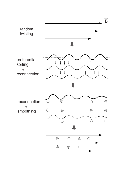
Figure 3: A new version of the mean-field dynamo. Turbulence twists the field lines into spirals, with each field line accumulating regions of right and left handed twisting. The turbulence is biased so that left-handed segments move down and right-handed segments move up. Reconnection, and a gradient in the strength of the spirals gives us new field lines with a net left-handed twist. The last step involves averaging over each field line, which is trivial but not part of the original picture, and reconnection to produce a new orthogonal field component.

In some sense equation (22) gives the minimal change in dynamo theory which respects conservation of magnetic helicity, since it leaves leaving ${\cal E}_{mf\perp}$ unchanged. That is, we assume that the backreaction from small scales affects only the component of the electromotive force along the direction of the large scale mean field. While this may seem unduly optimistic, we note that in the absence of any other large scale vector quantity, symmetry considerations alone should be sufficient grounds for this assumption. However, we are often concerned with circumstances where other large scale vectors are present, for example systems with differential rotation. In this case we are not guaranteed that $\langle{\bf v\times b}\rangle_{\perp}$ is unaffected by the inverse cascade. Obviously this is an important direction for future work.

There is another way in which equation (26) may fail to give the full magnetic helicity current. Equation (24) takes into account the perturbations in the large scale magnetic field driven by small scale velocties. However, fluctuations in the magnetic field also drive the velocity field. In conventional mean-field dynamo theory these considerations lead to replacing equation (14) with

$$\alpha_{il}\equiv\epsilon_{ijk}\left[\langle v_{j}\partial_{l}v_{k}\rangle-{\langle b_{j}\partial_{l}b_{k}\over 4\pi\rho}\rangle\right]\tau_{c}.$$ (28)

In our case equation (26) can be replaced by a symmetrized version, that is

$${\bf J}_{H}=-\tau_{c}\int{d^{3}{\bf r}\over 4\pi r}\epsilon_{lmn}\langle B_{k}\rangle\langle B_{l}\langle\partial_{k}\partial_{m}\left[\langle v_{i}({\bf x})v_{n}({\bf x}+{\bf r})-{b_{i}({\bf x})b_{n}({\bf x}+{\bf r})\over 4\pi\rho}\rangle\right].$$ (29)

This form fails to take into account the effects of shear from a large scale velocity field (like differential rotation). Given perfect symmetry between the dynamics of the velocity and magnetic fields, this term will be zero, regardless of any spatial symmetry-breaking effects. MHD turbulence tends to evolve towards this kind of symmetry. However, on the scale of the largest energy containing eddies, in realistic systems, we expect that differential shear, background gradients, and specific dynamical instabilities may all play a role, and all these effects will not respect the symmetry between magnetic and velocity fields. An example of an instability which will necessarily produce such an asymmetry is the magneto-rotational (or Balbus-Hawley) instability in accretion disks v59 ; c61 ; bh91 , which is discussed below.

Here we summarize some of the more important conclusions from these arguments.

1. The fluid helicity is largely irrelevant to flux generation, except when the field amplitude is very small, although it does affect flux transport.

2. This prescription eliminates turbulent dissipation for currents aligned with the large scale magnetic field, but continues to damp other current components. This is not a qualitative change in the role of turbulent damping for most field configurations, but does imply that force-free large scale fields are protected against turbulent dissipation.

3. The anomalous magnetic helicity current, $j_{H}$, depends on $\langle([{\bf B}\cdot\nabla]{\bf v})({\bf B}\cdot[\nabla\times{\bf v}])\rangle$, which has no particular relationship to the fluid helicity and is parity invariant. Rather than violating spatial symmetry along all three principal axes, a successful dynamo can result from a situation where only two out of three directions have broken symmetries. An example of this is differential rotation in a vertically uniform cylinder.

4. The ‘$\alpha-\Omega$’ dynamo has an analog in this new theory, which gives a similar growth rate, but which does not depend on any background vertical structure. (The analogous effect is provided by vertical gradients in $\langle{\bf B}\rangle$.) In an accretion disk, the success of the dynamo is tied to the outward transport of angular momentum vc01 .

5. The analog of the ‘$\alpha^{2}$’ dynamo of conventional theory has the difficulty that the turbulent dissipation term is of the same order as the driving term resulting from magnetic helicity transport. This does not imply that this kind of dynamo is impossible, but configurations with force-free, or nearly force-free, fields are strongly favored.

6. The analog of the ‘$\alpha-\Omega$ dynamo has a strong vertical magnetic helicity current, which has the same sign as $-\partial_{r}\Omega(r)$, i.e. towards $\hat{z}$ for an accretion disk and $-\hat{z}$ for a star like the Sun. This implies the necessity for magnetic helicity ejection at the system boundaries. While the energy budget for this is small compared to the energy budget of the dynamo in an accretion disk, it represents an unsolved aspect of the dynamo physics.

We note that the ejection of magnetic helicity from rotating systems as a necessary part of the dynamo process has been suggested by other authors bf00a ; bf00b , although the terms of the discussion were somewhat different. In particular, they were concerned with removing the magnetic helicity constraint by removing the magnetic helicity. Although realistic systems can work this way, there is no fundamental reason why the magnetic helicity can’t circulate within a closed system and produce a dynamo effect by being carried by large scale fields in one part of the system and eddy scale fields in another.

4 Applying and Testing the Theory

Both reconnection and the dynamo are the subject of intensive experimental research. Magnetic reconnection is being studied on several dedicated experiments around the world (MRX, TS3/4, SSX, VTF). In each experiment, magnetized loops are generated and merged. At present, the physical scales of such experiments are 0.1 to 1 m and the Lundquist number is about 1000. Sophisticated diagnostics are used to get plasma and magnetic field parameters in these experiments. This enables testing theoretical predictions. The direct relation between those experiments and astrophysics is complicated by the fact that some of the effects that are important in laboratory, e.g. anomalous resistivity, may not be important in conditions of astrophysical plasma, e.g. interstellar gas.

Dynamo experiments, e.g. using liquid sodium, are mostly focused on the reproduction of the dynamo effect for the low Lundquist numbers. In this regime, neither reconnection nor magnetic helicity are expected to provide strong constraints on the evolution of the experiments.

On the other hand, numerical simulations are a valuable source of information for mean-field dynamo theory. We have already discussed their role in undermining the conventional approach to this topic. It is also important to note that there are a large number of simulations which seem to show the operation of a successful dynamo, in the sense that they demonstrate the growth of a magnetic field with a significant component at large spatial scales. These are the simulations of magnetized, ionized accretion disks (e.g. hb91 ; hgb95 ; hgb96 ; shgb96 ; bnst95 ; bnst96 see also bh98 ; hb99 for a review) which are subject to the magneto-rotational instability. These simulations include extremely simplified physics and cover a limited set of spatial scales and geometries. Nevertheless, they agree in a number of important aspects, namely:

1. Any magnetic seed field undergoes substantial amplification to a final state which is (apparently) independent of initial conditions. In this state the magnetic field pressure is a few percent of the gas pressure and the dimensionless ‘viscosity’, $\alpha_{SS}$ is about half of this ratio. A large fraction of the magnetic energy is contained in a large scale field with a domain size which is a large fraction of the simulation box size. This large scale field is not static, but varies on time scales of tens of shearing times, a feature which seen in all of the simulations cited above.

2. The growth in field strength is rapid, i.e. a significant fraction of the shear rate, even when the field is weak. The growth is several times slower for an initially azimuthal field, where the amplification depends on dynamo action, as for an initially vertical field, where the amplification can simply reflect the linear growth of the instability, which generates azimuthal field, but the point remains true in either case.

3. The magnetic field pressure in the saturated state is not a constant fraction of the ambient pressure, but varies from a small fraction at the midplane (for models with vertical structure) to a value comparable to the gas pressure a few scale heights away from the midplane. This effect is particularly dramatic in the recent simulations of Miller and Stone ms00 . This distribution does not seem to be due to magnetic buoyancy shgb96 , that is, the fields are mostly generated locally. The time averaged magnetic stress ($\langle B_{r}B_{\theta}\rangle$) is somewhat more uniform.

4. The dynamo persists when vertical gravity is turned off, although the simulations are slightly different in this case hb92 ; hgb95 .

A possible interpretation of these results is that the simulations are showing a chaotic dynamo b50 ; k67 , in which turbulent stretching of embedded magnetic field lines results in a runaway amplification of the magnetic field. One problem with this is that the accretion disk simulations are unique in generating substantial magnetic field energy on scales much larger than the typical eddy size. Simulations of MHD turbulence in a box typically produce magnetic field structure whose energy spectrum peaks on scales slightly smaller  than a typical eddy scale and with a total energy density which is a (large) fraction of the kinetic energy density. At longer wavelengths the magnetic energy density falls, although slowly. Another point is that the vertical distribution of magnetic energy is not simply a reflection of local conditions, but seems to show some sort of global field evolution. The obvious conclusion is that some sort of large scale dynamo effect is being produced in the simulations, as a consequence of the Balbus-Hawley instability. Since there has been no attempt to look specifically at the flow of magnetic helicity, it is difficult to know whether to ascribe the dynamo effect to a locally produced fluid helicity (in which case the dynamo should slow down as the resolution is increased) or to a turbulently driven magnetic helicity current. The dynamo growth rate does not appear to slow down in the higher resolution studies, but this has not been examined critically. Further study of these simulations should allow testing of the notion that the turbulently driven magnetic helicity current is playing a critical role in these simulations.

There is one indirect test which has already been performed. Equation (27) can be used to show, via integration by parts, that the sign of the magnetic helicity current depends on the direction of angular momentum transport. Reversing the sign of the magnetic helicity current has the effect of turning off the dynamo. One simple numerical experiment is to conduct a simulation in which the angular momentum current flows in the opposite direction. This has been done hgb96 by turning off the centrifugal force term, so that the turbulence is driven only by a kind of magnetized Kelvin-Helmholtz instability. The dynamo effect was suppressed and the magnetic field decayed away, after an initial burst of growth. This simulation had a limited dynamic range, so that all the eddies were dominated by the local shear. Consequently, the elimination of the dynamo effect led to a complete suppression of the magnetic field through azimuthal stretching and radial mixing.

There has been a recent attempt to combine shear with an asymmetrically driven turbulence bbs01 to produce a non-heliacal dynamo. The results were disappointing. The expected correlation between the magnetic helicity flux and the velocity correlation seen in equation (27) was found, but the magnetic helicity flux was largely divergenceless and there was no clear correlation between the its small divergence and the electromotive force. This may have been due to the boundary conditions, which forced a return loop of magnetic flux within the box. Clearly further numerical experiments would be useful.

Assuming that we can understand the conceptual basis of accretion disk dynamos, it should be possible to construct a useful mean-field theory that incorporates transport effects and allows us to predict the dynamics of accretion disk fields. This model will need to incorporate the effects of fluctuations in the electromotive force vb97 . In the conventional mean-field dynamo theory such fluctuations have been shown to be capable of driving a mean-field dynamo in the absence of any average helicity. Their role in the modified version of mean-field dynamo theory is not yet understood. Such a model would be useful for building models of disks that incorporate both realistic local physics and MHD turbulence. A similar effort should be made for stellar dynamos, although there has been, as yet, no progress in this direction. There has been work on the galactic dynamo k02 which incorporates the notion of magnetic helicity current, including the term given in equation (26).

Much less progress has been made in numerical simulations of stochastic reconnection. This is particularly unfortunate since magnetic reconnection is one of the most fundamental properties of the magnetic field dynamics in the conducting fluid, and its applications are not limited to its consequences for astrophysical dynamos. In fact, reconnection is likely to be extremely important for the dynamics of the advection dominated flows, star formation, propagation (see cly02 ) and acceleration (see dl00 ; dl01 ) of cosmic rays, dynamics of charged dust ly02 . Direct study of the reconnection layer is difficult as both very small scales (turbulent microscales comparable to the current sheet thickness) and large scales (the contact region scale) are present in the problem. The requirement that we evolve structures at all scales over the whole broad reconnection region suppress any hope that adaptive mesh codes would be very helpful. Nevertheless, simple diagnostics may be used to distinguish fast stochastic reconnection from the Sweet-Parker model. For instance, using MHD simulations we can measure currents $J$, magnetic fields $B$ and velocities $v$. If we divide $\langle J^{2}[(B\cdot\nabla)B\cdot v]^{2}\rangle$ by $\langle J^{2}(\nabla\times B)^{2}\rangle$ then we have a measure of the rms magnetic field across a typical current sheet times the speed with which it is expelled. An approximate measure of reconnection speed can then be obtained by dividing the result by $\langle(J\times B)^{2}\rangle/\langle J^{2}\rangle$ and taking the square root. Although reconnection rates for low Lundquist numbers are not so different for the Sweet-Parker and stochastic reconnection models, the scaling of the reconnection rates with the Alfven velocity are very different. This gives some hope that the stochastic reconnection model can be tested before long.

5 Discussion and Summary

It is not possible to understand the astrophysical dynamo and dynamics of magnetized astrophysical plasmas without understanding how magnetic fields evade the topological constraints imposed by flux-freezing. This obviously includes the problem of reconnection, but also the more subtle difficulty posed by magnetic helicity conservation. Here we have compared traditional approaches to the problem of magnetic reconnection and the mean-field dynamo with new approaches based on an explicit recognition of the role geometry plays in both these problems. In fact, one of the more striking aspects of stochastic reconnection model lv99 is that the global reconnection speed is relatively insensitive to the actual physics of reconnection. Equation (8) only depends on the nature of the turbulent cascade. In the end, reconnection can be fast because if we consider any particular flux element inside the contact volume, assumed to be of order $L_{x}^{3}$, the fraction of the flux element that actually undergoes microscopic reconnection vanishes as the resistivity goes to zero. This is turn implies that reconnection is not tightly coupled to electron heating. More generally, the results presented here suggest that, in most cases, microphysics is irrelevant to the dynamo process.

Although objections to conventional dynamo theory tend to conflate the issues of reconnection and magnetic helicity conservation, these are, in fact, two separate problems, for which we have proposed two separate resolutions. Taken together, they imply that astrophysical dynamos are capable of operating in a broad range of circumstances. However, it is important to remember that they stand separately. Conventional dynamo theory is not rescued by assuming rapid reconnection, although it requires it. Conversely, the use of equations (22) and (26) to describe dynamo activity do not require stochastic reconnection, but only that some model of fast reconnection work.

Our main conclusions are as follows:

• The rate of magnetic reconnection is increased dramatically in the presence of a stochastic component to the magnetic field. Even when the turbulent cascade is weak the resulting reconnection speed is independent of the Ohmic resistivity. However, it is extremely sensitive to the level of noise. This may explain the variable rates of magnetic reconnection seen in the solar corona. It also implies that laminar flow patterns that drive a magnetic helicity current may still require some level of local turbulence in order to drive a large scale dynamo.

• The argument that the rapid rise of random magnetic field associated with dynamo action results in the suppression of dynamo ka92 is untenable since the increase of the random component of the magnetic field increases the reconnection rate. We conclude that dynamo is a self-regulating process.

• Conventional mean-field dynamo theory, which does not account for the conservation of magnetic helicity is ill-founded. The suggested modification of the mean-field dynamo equations allow us to account for results of numerical sumulations and make the theory, for the first time ever, self-consistent.

Acknowledgements. AL and JC acknowledge the support of NSF grant NSF AST-0125544. ETV acknowledges the support of NSF grant AST-0098615. AL thanks the LOC for the financial support.

References

- (1) J. W. Armstrong, B.J. Rickett, S.R. Spangler: Astrophys. J. 443, 209 (1995)
- (2) S. A. Balbus, J. F. Hawley: Astrophys. J. 376, 214 (1991)
- (3) S. A. Balbus, J. F. Hawley: Rev. Mod. Phys. 70, 1 (1998)
- (4) D. Balsara: Rev.Mex.A.A. 9, 9 (2000)
- (5) G. K. Batchelor: Proc. R. Soc. Lond. A201, 405 (1950)
- (6) A. Bhattacharjee, E. Hameiri: Phys. Rev. Lett. 57, 206 (1986)
- (7) D. Biskamp: Phys. Lett. A 105, 124 (1984)
- (8) D. Biskamp: Phys. Fluids 29, 1520 (1986)
- (9) D. Biskamp: Astrophys. & Sp. Sci. 242, 165 (1996)
- (10) E. G. Blackman, G. B. Field: Astrophys. J. 534, 984 (2000)
- (11) E. G. Blackman, G. B. Field: Mon. Not. R. A. S. 318, 724 (2000)
- (12) D. Bohm, E. H. S. Burhop, H. S. W. Massey: In: The Characteristics of Electrical Discharges in Magnetic Fields, ed. by A. Guthrie & R.K. Wakerling (New York: McGraw Hill 1949) pp. 77-86
- (13) A. Brandenburg: Astrophys. J. 550, 824 (2001)
- (14) A. Brandenburg, Å. Nordlund, R. F. Stein, U. Torkelsson: Astrophys. J. 446, 741 (1995)
- (15) A. Brandenburg, Å. Nordlund, R. F. Stein, U. Torkelsson: Astrophys. J. Lett. 458, 45 (1996)
- (16) A. Brandenburg, E. Zweibel: Astrophys. J. 448, 734 (1995)
- (17) A. Brandenburg, A. Bigazzi, K. Subramanian: Mon. Not. R. Astron. Soc. 325(2), 685 (2001)
- (18) S. V. Bulanov, J. Sakai, S. I. Syrovatskii: Sov. J. Plasma Phys. 5(2), 157 (1979)
- (19) F. Cattaneo, D. W. Hughes: Phys. Rev. E, 54, 4532 (1996)
- (20) F. Cattaneo, S. I. Vainshtein: Astrophys. J. Lett. 376, 21 (1991)
- (21) S. Chandrasekhar: Hydrodynamic and Magnetohydrodynamic Stability(Oxford: Oxford University Press 1961)
- (22) J. Cho, E. T. Vishniac: Astrophys. J. 538, 217 (2000a)
- (23) J. Cho, E. T. Vishniac: Astrophys. J. 539, 273 (2000b)
- (24) J. Cho, A. Lazarian, E. T. Vishniac: Astrophys. J. 564, 291 (2002)
- (25) J. Cho, A. Lazarian, E. T. Vishniac: Astrophys. J. Lett. 566, 49 (2002)
- (26) J. Cho, A. Lazarian, H. Yan: In: Seeing through dust, eds,ASP conf. ser. Russ Taylor, Tom Landecker, and Tony Willis, (2002)
- (27) K. P. Dere: Astrophys. J. 472, 864 (1996)
- (28) E. M. de Gouveia Dal Pino, A. Lazarian: Astrophys. J. 536, 31 (2000)
- (29) E. M. de Gouveia Dal Pino, A. Lazarian: Astrophys. J. 560, 358 (2001)
- (30) U. Frisch, A. Pouquet, J. Leorat, A. Mazure: J. Fluid Mech. 68, 769 (1975)
- (31) H. P. Furth, J. Killeen, M. N. Rosenbluth: Phys. Fluids 6, 459 (1963)
- (32) G. A. Glatzmaier, P. H. Roberts: Nature 377, 203 (1995)
- (33) P. Goldreich, S. Sridhar: Astrophys. J. 438, 763 (1995)
- (34) A. Gruzinov, P. H. Diamond: Phys. Rev. Lett. 72, 1651 (1994)
- (35) A. Gruzinov, P. H. Diamond: Phys. Plasmas 3, 1853 (1996)
- (36) J. F. Hawley, S. A. Balbus: Astrophys. J. 376, 223 (1991)
- (37) J. F. Hawley, S. A. Balbus: Astrophys. J. 400, 610 (1992)
- (38) J. F. awley, S. A. Balbus: Phys. Plasmas 6(12), 4444 (1999)
- (39) J. F. Hawley, C. F. Gammie, S. A. Balbus: Astrophys. J. 440, 742 (1995)
- (40) J. F. Hawley, C. F. Gammie, S. A. Balbus: Astrophys. J. 464, 690 (1996)
- (41) P. Iroshnikov: Astron. Zh. 40, 742 (1963) [Sov. Astron. 7, 566 (1963)]
- (42) H. Ji: Phys. Rev. Lett. 83, 3198 (1999)
- (43) S. R. Kane, K. Hurley, J. M. McTiernan, M. Boer, M. Niel, T. Kosugi, M. Yoshimori: Astrophys. J. 500, 1003 (1998)
- (44) A. P. Kazantsev: JETP 53, 1806 (1967)
- (45) E.-J. Kim, P. H. Diamond: Astrophys. J. 556, 1052 (2001)
- (46) N. Kleeorin, D. Moss, I. Rogachevskii, D. Sokoloff: Astro. & Astrophys. Lett. 361, 5 (2000)
- (47) N. Kleeorin, D. Moss, I. Rogachevskii, D. Sokoloff: Astro. & Astrophys. 387, 453 (2002)
- (48) R. Kraichnan: Phys. Fluids 8, 1385 (1965)
- (49) F. Krause, K. H. Radler: Mean-Field Magnetohydrodynamics and Dynamo Theory (Oxford: Pergamon Press 1980)
- (50) R. M. Kulsrud, S. W. Anderson: Astrophys. J. 396, 606 (1992)
- (51) A. Lazarian: Astron. & Astrophys. 264, 326 (1992)
- (52) A. Lazarian, D. Pogosyan: Astrophys. J. 537, 720 (2000)
- (53) A. Lazarian, E. T. Vishniac: Astrophys. J. 517, 700 (1999)
- (54) A. Lazarian, E. T. Vishniac: Revista Mexicana de Astronomia y Astrofisica 9, 55 (2000)
- (55) A. Lazarian, H. Yan: Astrophys. J. 000, (2002)
- (56) A. Lazarian, E. T. Vishniac, J. Cho: in preparation (2002)
- (57) R. J. Leamon, C. W. Smith, N. F. Ness, W. H. Matthaeus: J. Geophys. Res. 103, 4775 (1998)
- (58) Z. W. Ma, A. Bhattacharjee: J. Geophys. Res. 101, 2641 (1996)
- (59) W. H. Matthaeus, S. L. Lamkin: Phys. Fluids 28, 303 (1985)
- (60) M. Meneguzzi, U. Frisch, A. Pouquet: Phys. Rev. Lett. 47, 1060 (1981)
- (61) K. A. Miller, J. M. Stone: Astrophys. J. 534, 398 (2000)
- (62) H. K. Moffatt: Magnetic Field Generation in Electrically Conducting Fluids, (Cambridge: Cambridge University Press 1978)
- (63) K. Naidu, J. F. McKenzie, W. I. Axford: Ann. Geophysicae 10, 827 (1992)
- (64) E. N. Parker: J. Geophys. Res. 62, 509 (1957)
- (65) E. N. Parker:Cosmical Magnetic Fields (Oxford: Clarendon Press 1979)
- (66) E. N. Parker: Astrophys. J. 401, 137 (1992)
- (67) H. E. Petschek: ‘Magnetic Field Annihilation’ In: The Physics of Solar Flares, ed. by W.H. Hess (Washington, DC, NASA Special Publications 50) pp. 425-439
- (68) E. Priest, T. Forbes: Magnetic Reconnection: MHD Theory and Applications (Cambridge: Cambridge University Press 2000)
- (69) M. Rees: Q. J. Roy. Astr. Soc. 28, 197 (1988)
- (70) M. A. Shay, J. F. Drake: Geophys. Res. Lett. 25(20), 3759 (1998)
- (71) M. A. Shay, J. F. Drake, R. E. Denton, D. Biskamp: J. Geophys. Res. 103, 9165 (1998)
- (72) M. A. Shay, J. F. Drake, B. N. Rogers, R. E. Denton: Geophys. Res. Lett. 26(14), 2163 (1999)
- (73) J. M. Stone, J. F. Hawley, C. F. Gammie, S. A. Balbus: Astrophys. J. 463, 656 (1996)
- (74) S. Stanimirovic, A. Lazarian: Astrophys. J. Lett. 551, 53 (2002)
- (75) H. R. Strauss: Astrophys. J. 326, 412 (1988)
- (76) W. T. Stribling, W. H. Matthaeus, S. Ghosh: J. Geophys. Res. 99, 2567 (1994)
- (77) W. T. Stribling, W. H. Matthaeus, S. Oughton: Phys. Plasmas 2, 1437 (1995)
- (78) P. A. Sweet: ‘The Neutral Point Theory of Solar Flares’. In: IAU Symp. 6, Electromagnetic Phenomena in Cosmical Plasma. ed. by B. Lehnert (New York: Cambridge Univ. Press 1958) pp.123-134
- (79) J. B. Taylor: Phys. Rev. Lett. 33, 1139 (1974)
- (80) S. I. Vainshtein, E. N. Parker, R. Rosner: Astrophys. J. 404, 773 (1993)
- (81) E. P. Velikhov: Sov. Phys. JETP Lett. 35, 1398 (1959)
- (82) E. T. Vishniac, A. Brandenburg: Astrophys. J. 475, 263 (1997)
- (83) E. T. Vishniac, J. Cho: Astrophys. J. 550, 752 (2001)
- (84) E. T. Vishniac, A. Lazarian: Astrophys. J. 511, 193 (1999)
- (85) X. Wang, Z. W. Ma, A. Bhattacharjee: Phys. Plasmas 3(5), 2129 (1996)
- (86) M. Yamada, H. Ji, S. Hsu, T. Carter, R. Kulsrud, F. Trintchouk: Phys. Plasmas 7(5), 1781 (2000)
- (87) E. Zweibel: Phys. Plasmas 5, 247 (1998)
- (88) E. Zweibel, A. Brandenburg: Astrophys. J. 478, 563 (1997)