A FUSE Survey of Interstellar Molecular Hydrogen in Translucent Clouds

Abstract

We report the first ensemble results from the FUSE survey of molecular hydrogen in lines of sight with $A_{V}$ $\gtrsim$ 1 mag. We have developed techniques for fitting computed profiles to the low-$J$ lines of H₂, and thus determining column densities for $J$ = 0 and $J$ = 1, which contain $\gtrsim$99% of the total H₂. From these column densities and ancillary data we have derived the total H₂ column densities, hydrogen molecular fractions, and kinetic temperatures for 23 lines of sight. This is the first significant sample of molecular hydrogen column densities of $\sim$10²¹ cm^-2, measured through UV absorption bands. We have also compiled a set of extinction data for these lines of sight, which sample a wide range of environments. We have searched for correlations of our H₂-related quantities with previously published column densities of other molecules and extinction parameters. We find strong correlations between H₂ and molecules such as CH, CN, and CO, in general agreement with predictions of chemical models. We also find the expected correlations between hydrogen molecular fraction and various density indicators such as kinetic temperature, CN abundance, the steepness of the far-UV extinction rise, and the width of the 2175 Å bump. Despite the relatively large molecular fractions, we do not see the values greater than 0.8 expected in translucent clouds. With the exception of a few lines of sight, we see little evidence for the presence of individual translucent clouds in our sample. We conclude that most of the lines of sight are actually composed of two or more diffuse clouds similar to those found toward targets like $\zeta$ Oph. We suggest a modification in terminology to distinguish between a “translucent line of sight” and a “translucent cloud.”

1 Introduction

Molecular hydrogen is the most abundant molecule in the interstellar medium, dominating the composition of the dense clouds that contain most of the mass. Even in diffuse clouds, H₂ is present, containing from 10^-6 to about half of the total hydrogen nuclei (e.g., Spitzer, Cochran, & Hirshfeld 1974; Shull & Beckwith 1982). Clearly, a full understanding of the physics and chemistry of the ISM requires a detailed knowledge of molecular hydrogen.

As a homonuclear molecule, H₂ has no dipole moment and hence no allowed rotational or vibrational transitions in the radio and infrared spectral regions. With the exception of forbidden quadrupole transitions in the infrared, which can be seen in emission in regions heated by radiation or shocks (Timmermann et al. 1996), or, in rare cases, in absorption when sufficiently high column densities are probed (Lacy et al. 1994), the only way to observe cold interstellar H₂ is through its electronic transitions in the far ultraviolet.

The Lyman (B$\rightarrow$X) and Werner (C$\rightarrow$X) bands lie in the spectral region between about 844 Å and 1126 Å. The moment of inertia for this low-mass molecule is small, resulting in widely separated rotational lines which are easily resolved. As a result, the far-UV spectrum of any reddened star is dominated by a wealth of H₂ absorption bands. For a summary of the spectra of these bands, see Morton & Dinerstein (1976) or Barnstedt et al. (2000).

Previous far-UV observations of H₂ absorption have been conducted by various short-term missions, including sounding rockets (Carruthers 1970 – the first detection of H₂ in space); the Hopkins Ultraviolet Telescope (e.g., Blair, Long, & Raymond 1996); ORFEUS (e.g., Barnstedt et al. 2000); and IMAPS (e.g., Jenkins & Peimbert 1997). But by far the most extensive previous observations of far-UV H₂ absorption were performed by the Copernicus satellite, which provided the first general quantitative studies of interstellar H₂ as well as a wealth of information on its formation, its abundance, and its excitation in space (e.g., Spitzer et al. 1973; Spitzer, Cochran, & Hirshfeld 1974; Spitzer & Zweibel 1974; Jura 1975a,b; for summaries, see Spitzer & Jenkins 1975 and Shull & Beckwith 1982). The Copernicus work culminated in a survey of molecular and atomic hydrogen for 109 stars (Savage et al. 1977; Bohlin, Savage, & Drake 1978).

The Far Ultraviolet Spectroscopic Explorer (FUSE) instrument is well suited for observations of the H₂ bands in absorption, and studies of H₂ have been a longstanding goal of the FUSE mission (Moos et al. 2000). FUSE covers the wavelength region from the Lyman limit at 912 Å to about 1187 Å  with spectral resolving power of about $\lambda$/$\Delta$$\lambda$ $\approx$ 20,000. The throughput of FUSE has been specifically maximized in the middle of the Lyman band (around 1050 Å), providing by far the most sensitive instrument yet available for observing cold H₂ in the ISM. For a full description of the FUSE mission and instrumental performance, see Moos et al. (2000) and Sahnow et al. (2000), respectively.

A subset of the FUSE Science team is conducting a program to study H₂ in the densest clouds accessible, the so-called “translucent clouds” (van Dishoeck & Black 1988). These clouds are defined as being optically thick (with total extinctions A_V $\gtrsim$ 1 mag) yet still sufficiently transparent as to allow optical and UV absorption-line measurements of interstellar atoms, ions, and molecules. The upper limit on extinction for a translucent cloud is usually considered to be about A_V $\approx$ 5 mag; beyond that limit there is usually not enough flux to allow high-resolution visible-wavelength spectroscopy, much less ultraviolet spectroscopy, which is always hindered by the rise in dust extinction at short wavelengths. Hence the goal of our program has been to observe and survey molecular hydrogen in translucent clouds, going as far as possible in the direction of maximum extinction, with the hope of penetrating clouds with A_V as high as 5 magnitudes. In doing so, we planned to extend the Copernicus-based surveys of Savage et al. (1977) and Bohlin et al. (1978) to greater extinctions and denser clouds.

More specifically, the goals of the FUSE translucent cloud H₂ survey include:

$\bullet$ Measuring total gas column densities, to help in determining interstellar gas-phase depletions and chemistry.

$\bullet$ Studying the relationship between H₂ and dust extinction, as an aid in assessing H₂ formation models as well as extending correlations between extinction and H₂ column density, sometimes used to estimate cloud masses.

$\bullet$ Assessing the molecular fraction $f_{\rm H2}$ = 2$N$(H₂)/[2$N$(H₂) + $N$(H I)] and its relationship to dust extinction and other line-of-sight characteristics.

$\bullet$ Measuring gas kinetic temperatures ($T_{01}$) from the ratio of $J$ = 1 to $J$ = 0 rotational states, and assessing the corrrelation of $T_{01}$ with other interstellar quantities.

$\bullet$ Extending direct measurements of the CO/H₂ correlation through UV absorption features of CO. This correlation is widely used to assess total masses of molecular clouds, but is currently based largely on CO abundances derived from mm-wave radio observations which do not necessarily sample the same material as H₂ in absorption, and indirect H₂ abundances estimated from dust extinction measures.

$\bullet$ Assessing cloud physical conditions such as density and radiation field intensity by analyzing the excitation of high rotational states ($J$ = 2 and greater).

$\bullet$ Comparing H₂ absorption measures from FUSE with infrared emission often attributed to complex molecules (e.g., PAHs) as measured by the IRAS mission.

$\bullet$ Measuring the abundance of HD in order to infer information on the D/H ratio.

As will be seen later in this paper, all but the last three goals have now been met. We note also that UV absorption-line CO data do not yet exist for all of our program stars, so more progress on the CO/H₂ correlation will come later.

Two papers on FUSE observations of H₂ in translucent clouds have already been published (Snow et al. 2000 [Paper I]; Rachford et al. 2001 [Paper II]). In addition to our translucent cloud H₂ survey, another subset of the FUSE Science Team is conducting a general survey of molecular hydrogen in diffuse lines of sight, including Galactic stars with relatively little reddening, stars at high Galactic latitude, Magellanic Cloud stars (Tumlinson et al. 2002), and H₂ in the lines of sight toward other extragalactic sources such as AGNs (Shull et al. 2000).

The rest of the paper is organized as follows: in § 2 we describe the criteria for selecting target stars for the FUSE H₂ survey, along with comments on the stars chosen; in § 3 we give details of the observations and data reduction and analysis; in § 4 we summarize the results; and in § 5 we discuss these results and their implications.

2 Target Selection and Stellar Properties

2.1 General Criteria for Selecting Target Stars

Unlike the case of the diffuse H₂ survey, which has been able to use spectra obtained by FUSE for other programs (e.g., the survey of stellar winds in OB stars; the survey of hot gas in the Galactic halo; and the survey of interstellar gas at high latitudes and along lines of sight toward the Magellanic Clouds and other galaxies), our sole source of data comes from stars we observe specifically for our program on translucent cloud lines of sight. No one observes heavily reddened stars unless absolutely necessary, because the dust extinction acts to increase the observing time needed, particularly at short wavelengths. Thus, we had to conserve observing time and be as careful as possible in choosing our target stars while seeking to fulfill our basic criteria.

The result was a list of 45 stars; 31 assigned to FUSE program P116, 4 assigned to Q101, 9 assigned to P216, and one target (HD 24534) added from the personal program of one of us (T.P.S.; P193). Of these 45 stars, 25 had been observed through June 2001, and 23 are included in this paper.

The selection of target stars for the FUSE translucent cloud H₂ survey program was based on several criteria:

$\bullet$ Maximizing the total extinction probed;

$\bullet$ Exploring lines of sight known to have a wide range of extinction characteristics such as $R_{V}$ (the ratio of total to selective extinction) and the extinction parameters defined by Fitzpatrick & Massa (1986, 1988, 1990) on the basis of IUE data;

$\bullet$ Relative simplicity of line-of-sight velocity structure based on high resolution observations of K I, Na I, and CH;

$\bullet$ Availability of (or feasibility of obtaining) ancillary data on optical interstellar lines of atomic and molecular species not observed in the FUSE passband (including ultra-high resolution spectra for velocity structure analysis), and the availability (or feasibility of obtaining) infrared spectra of both gas-phase and solid-state absorption features.

The first of these criteria was the most critical, due to the trade-off between maximizing dust extinction and finding stars with sufficient far-UV flux to be observable with FUSE within reasonable exposure times. Thus, we explored known UV fluxes for candidate stars, in most cases having to extrapolate to shorter wavelengths from the IUE cutoff at about 1170 Å. The extrapolations were based on a combination of the known flux in the IUE band, the spectral type and instrinsic flux distribution of the star, and the shape of the UV extinction curve.

In our initial selection of targets we drew heavily upon the IUE-based ultraviolet extinction curve survey of Fitzpatrick & Massa (1986, 1988, 1990) and several papers on optical interstellar absorption lines, both atomic and molecular (e.g., van Dishoeck & Black 1989; Gredel, van Dishoeck, & Black 1993). We eliminated stars known to have complex line-of-sight Doppler structure due to multiple clouds. However, we found that this distinction was almost futile, as nearly every line of sight turned out to have complex structure when examined at sufficiently high spectral resolution. For example, the star we chose to analyze for our first paper from this program, HD 73882 (Paper I), turned out to have no fewer than 21 identifiable Doppler components in the ultra-high resolution spectra of optical interstellar lines due to K I and Na I.

One of us (D.E.W.) has led a program to obtain very high-resolution optical spectra of our FUSE candidates, and has succeeded in obtaining spectra at resolving powers of $\lambda$/$\Delta$$\lambda$ $\geq$ 150,000 in most cases. The results will appear in a separate paper (D. E. Welty et al. 2002, in preparation) while being made available to us as we analyze the FUSE H₂ spectra. But, these high-resolution spectra are not very important for the current survey, since we include here only the two lowest rotational states of H₂, whose absorption lines are damped and which therefore can be analyzed accurately without concern for the detailed velocity structure. We do, however, reference the optical spectra in a few cases.

Table 2 provides ancillary data, where available, on carbon-based molecular species for the stars listed in Table 1. Additional data regarding the CH component structure will be discussed in § 5.1. We plan to supplement Table 2 by performing our own ground-based observations of various atomic and molecular species. We expect especially to emphasize infrared spectroscopy in this effort, in order to obtain data on both gas-phase and solid-state absorption features such as those due to CO, water ice, and the 3.4-$\micron$ hydrocarbon feature.

2.2 Extinction properties

The fundamental quantities used to categorize dust extinction along a line of sight are $E(B-V)$ and $R_{V}$ = $A_{V}$/$E(B-V)$, where $A_{V}$ is the total visual extinction in magnitudes. Since $E(B-V)$ is also expressed in magnitudes, $R_{V}$ is unitless. The quantity $E(B-V)$, or color excess, represents the amount of reddening along a line of sight and gives a measure of the amount of dust and gas. The quantity $R_{V}$, or total-to-selective extinction ratio, gives a measure of the size of dust grains, and is a convenient single parameter for describing the overall shape of extinction curves (Cardelli, Clayton, & Mathis 1989). The detailed shape of the UV extinction curve also carries considerable information. We discuss these extinction properties in the following sections.

2.2.1 $E(B-V)$

The determination of the $E(B-V)$ color excess is relatively straightforward for early-type stars. The intrinsic $(B-V)_{0}$ colors for O and B stars vary slowly as a function of spectral type, minimizing errors due to inaccurate typing and variations in $R_{V}$. Table 3 gives our adopted values. In most cases, these values come from either an analysis of the upper main sequences of OB associations, or simply from a comparison of the observed colors to tabulated intrinsic colors for a given spectral type. The differences between the various references for a given star are typically only a few hundredths of a magnitude at worst. This is comparable to the differences between different lists of intrinsic colors, and not much greater than the photometric uncertainties themselves. In the case of the Be star HD 110432, the value quoted in Table 3 includes a correction to the observed $E(B-V)$ to allow for the emission line behavior.

2.2.2 $R_{V}$

The situation with regards to $R_{V}$ is not as simple. Whatever the method, measuring $R_{V}$ requires more difficult observations with much greater calibration problems. We will exploit three methods for estimating $R_{V}$ in the present work.

If a star does not show excess infrared emission (e.g. Be stars or other stars with circumstellar material), an extrapolation of infrared color excesses to infinite wavelength yields an estimate of $R_{V}$. In the method developed by Martin & Whittet (1990), the near-infrared extinction curve takes the form,

$$\frac{E_{\lambda-V}}{E_{B-V}}=e\lambda^{-\alpha}-R_{V}.$$ (1)

The infrared extinction in the range 0.9–4.8 $\mu$m has been expressed as

$$\frac{A_{\lambda}}{E_{B-V}}=e\lambda^{-\alpha},$$ (2)

where $e$ is the power-law amplitude, similar to the $c_{4}$ parameter of the UV extinction curves described in § 2.2.3, and $\lambda$ is given in $\mu$m. Martin & Whittet found that the power-law index, $\alpha$, rarely deviates from the average value of 1.8, even for material with $R_{V}$ far from the interstellar average of 3.1. Thus, to within the normalization provided by $e$, all extinction curves in the range $\lambda$ = 0.9–4.8 $\mu$m can be described by this universal curve. With the known quantities $E_{\lambda-V}$/$E_{B-V}$ and $\lambda^{1.8}$ as the ordinate and abscissa, respectively, we can fit a linear relation with slope $e$ and a $y$-intercept of $-R_{V}$. This allows us to apply Eq. 1 to cases where we only have 3 infrared measurements (or even 2 measurements, with much greater uncertainty). We have verified that in the cases where we have 4 or 5 measurements, the full form of Eq. 1 gives results consistent with the linearized form; i.e. $\alpha$ $\approx$ 1.8. Although Eq. 1 and 2 appear to hold for photometric bands from $I$ through $M$, we have limited our fits to the five available bands from $J$ through $M$. As Table 3 indicates, we generally had 3 or 4 bands to work with.

One complication of this method is that the colors of the stars must be corrected for reddening by comparison with a standard relationship as a function of spectral type. In absolute terms, the infrared colors $(J-V)_{0}$, $(H-V)_{0}$, etc. change much more rapidly with changing spectral type than $(B-V)_{0}$. The choice of the appropriate set of intrinsic colors, as well as the spectral type, leads to significant differences in the derived value of $R_{V}$. Many authors have used older intrinsic color-spectral type relationships such as that of Johnson (1966). However, one must interpolate to generate the appropriate $H-V$ colors, and the tables are incomplete for O stars. More recently, Wegner (1994) compiled a more complete set of intrinsic colors for O and B stars, and other similar calibrations exist.

We found infrared photometry in at least 2 filters for 19 of our 23 stars and performed fits to Eq. 1 based on intrinsic colors from both Johnson (1966) and Wegner (1994). In many cases, photometric uncertainties for a specific star were not given. Thus, in our error analysis, we assumed $\sigma$ = 0.03 for $JHK$, $\sigma$ = 0.05 for $LM$, and $\sigma$ = 0.04$E(B-V)$ for $E(B-V)$. The final statistical uncertainties on $R_{V}$ were then close to 0.2 in all cases.

In two cases, HD 110432 and HD 168076, we could not obtain reasonable fits to Eq. 1. HD 110432 is a Be star, so that we would not expect this method to work due to the distorted infrared colors. HD 168076 also shows emission lines. However, several other O stars in our sample also show emission lines, yet the infrared photometry closely follows the expected power law. We have noticed for this star that the infrared photometry from Thé et al. (1990) differs significantly from that given by Aiello et al. (1988), yet neither set of photometry obeys Eq. 1.

For the remaining stars with photometry in 4 or 5 filters and good fits, the differences between the two sets of intrinsic colors are large and systematic. The differences averaged 0.20, and in all cases the values of $R_{V}$ were smaller for the Wegner (1994) intrinsic colors.

For the 7 cases where previous authors have used this or a similar method (BD $+$31^∘ 643, HD 62542, HD 73882, HD 206267, HD 207198, HD 210121, and HD 210839), our values agree nearly exactly when we have used the same set of intrinsic colors. Considering that the differences in $R_{V}$ for the two different sets of intrinsic colors are smallest for the B stars, and that the Wegner (1994) calibration is much more complete for the O stars, we have accepted this calibration as the more accurate overall and give those values in Table 3.

The wavelength of maximum linear polarization generally correlates well with $R_{V}$, following the relationship

$$R_{V}=(5.6\pm 0.3)\lambda_{\rm max},$$ (3)

where $\lambda_{\rm max}$ is given in $\mu$m (Whittet & van Breda 1978). Combined with the uncertainties in determining $\lambda_{\rm max}$ (a few tenths of a percent to several percent), this method produces values of $R_{V}$ accurate to about 5–10%, similar to the uncertainties from the first method.

It is worth emphasizing that the relationship between $R_{V}$ and $\lambda_{\rm max}$ was calibrated in part from infrared photometry, so that this second method is not completely independent of the first. A further complication is that Eq. 3 may not always be satisfied. Recently, Whittet et al. (2001) found deviations from Eq. 3 within the Taurus dark clouds for a number of lines of sight, in the sense of larger than normal $\lambda_{\rm max}$ for normal values of $R_{V}$ derived from IR photometry.

Finally, one can estimate $R_{V}$ by comparing the ultraviolet extinction curves to standard curves. Again, this method requires calibration from other methods of determining $R_{V}$. A comparison of the shapes of extinction curves can be somewhat subjective. However, in an important set of papers, Fitzpatrick & Massa (1986, 1988, 1990) devised a six-parameter description of the ultraviolet curves that could reproduce the entire curve to within the observational errors. We discuss extinction curves in more detail in the following section, but the most useful correlation is between $R_{V}$ and the linear far-UV rise, the “$c_{2}$” parameter. The relationship derived by Fitzpatrick (1999) is

$$c_{2}=-0.824+4.717R_{V}^{-1}.$$ (4)

The typical scatter about this relationship is a few hundredths in $R_{V}^{-1}$, or $\sim$0.2 in $R_{V}$ for small values, and $\sim$0.5 for large values. Larger deviations occur for a few lines of sight. For example, the extinction curve for HD 62542 has an extremely steep far-UV rise, out of proportion with the rest of the curve (Cardelli & Savage 1988).

Unfortunately, in some cases, there are significant disagreements in $R_{V}$ derived from the different methods. However, in most cases the agreement between the methods is reasonable. The most direct method for the determination of $R_{V}$ is the method involving IR photometry, and we have such a determination for a majority of our targets. We have used this method as our primary source for $R_{V}$, using values from polarimetry and the extinction curves in that order to supplement the IR photometry. We then simply derive $A_{V}$ from the product of $R_{V}$ and $E(B-V)$ (Table 3). We have not included specific uncertainties on these values, but as we noted above, the typical statistical uncertainty on the photometric values of $R_{V}$ is 0.2. The resultant statistical uncertainties on $A_{V}$ are then typically 0.1–0.3. Systematic effects may be important as noted above in the discussion of the methods of determining $R_{V}$.

2.2.3 Extinction curves

As mentioned previously, Fitzpatrick & Massa (1986, 1988, 1990) devised a six-parameter scheme to describe the UV extinction curve in the IUE wavelength range, $\sim$1170–3200 Å. The six parameters include three that describe the central wavelength ($x_{0}$), width ($\gamma$), and height ($c_{3}$) of the 2175 Å bump, two that represent a linear background term ($c_{1}$ and $c_{2}$), and one that describes the far-UV curvature ($c_{4}$). With $x\equiv\lambda^{-1}$ in units of $\mu$m^-1, the function describing the extinction curves, $k$, is given by

$$k(x-V)=c_{1}+c_{2}x+c_{3}D(x;\gamma,x_{0})+c_{4}F(x),$$ (5)

where

$$D(x;\gamma,x_{0})=\frac{x^{2}}{(x^{2}-x_{0}^{2})^{2}+x^{2}\gamma^{2}},$$ (6)

and

$$F(x)=\left\{\begin{array}[]{lr}0.5392(x-5.9)^{2}+0.0564(x-5.9)^{3}&x\geq 5.9\\ 0&x<5.9\\ \end{array}\right.$$ (7)

The function $D(x;\gamma,x_{0})$ is the so-called Drude function (the absorption profile of a damped freely oscillating electron) and represents the 2175 Å bump. The far-UV curvature is described by the function $F(x)$. As previously noted, $c_{2}$ correlates well with $R_{V}$, and grain size. Table 4 gives previously published extinction curve parameters for most of our targets. In § 4.5 we will investigate various correlations involving these parameters.

2.3 Special line-of-sight characteristics

Many of the lines of sight are of special interest due to their location and/or environment. We give a brief overview of each line of sight in the following sections, including the mention of particularly interesting values from Tables 1–4.

2.3.1 BD $+$31^∘ 643

The binary system BD $+$31^∘ 643 lies within the cluster IC 348 and interstellar material associated with the cluster. The line of sight is only 8$\arcmin$ from the well studied line of sight toward o Per. However, the latter star lies in the background of IC 348 and its associated material (Sancisi et al. 1974). Snow et al. (1994) found a “composite” extinction curve, with contributions from material having a broad 2175 Å bump and steep far-UV rise, and from material having a narrow bump and shallow far-UV rise. Also, the authors noted very different molecular abundances in the two lines of sight: enhanced CH and CH⁺ column densities toward BD $+$31^∘ 643, and a reduced CN abundance. They concluded that star formation in this cluster has altered the physical and chemical state of the gas. Snow (1993) has argued that the enhanced CH⁺ column density is larger than would be expected from shock formation, and proposed a radiative formation mechanism due to a very strong UV radiation field.

BD $+$31^∘ 643 is surrounded by a circumstellar disk, only the second such disk ever directly imaged (Kalas & Jewitt 1997). Andersson & Wannier (2000) suggest that more then one magnitude (approximately half) of the total visual extinction may arise in this disk. This might lead to a composite extinction curve, and a single $R_{V}$ might not be an appropriate description of the line of sight.

2.3.2 HD 24534

This Be star is more commonly known as X Persei and has an X-ray-bright pulsar companion. However, the line of sight toward the pair intersects a molecular cloud, and the UV flux is among the largest known for a target with $A_{V}$ $>$ 1 mag. In fact, it was (barely) bright enough to be observed with Copernicus (Mason et al. 1976). They found log $N$(H₂) = 21.04, the largest such value obtained with Copernicus. The molecular fraction was also estimated to be very large (Snow et al. 1998), albeit the H₂ column density was rather uncertain.

2.3.3 HD 27778

This binary star lies within or just behind the Taurus-Auriga molecular cloud complex (Kenyon, Dobrzycka, & Hartmann 1994), sampling relatively low-extinction material in this complex (Whittet et al. 2001). Although fit parameters have not been published for the extinction curve, the curve depicted in Joseph et al. (1986) indicates greater-than-normal far-UV extinction, and a shallower-than-normal 2175 Å bump, characteristic of a “dense cloud” environment.

We note that while Joseph et al. (1986) reported an H I column density log $N$ = 21.59$\pm$0.11 from measurement of the Ly$\alpha$ line, at spectral type B3 V the Lyman-series interstellar lines will be strongly contaminated by stellar lines (Savage & Panek 1974; Shull & van Steenberg 1985; Diplas & Savage 1994).

2.3.4 HD 62542

HD 62542 lies in or just beyond the Gum nebula, and the line of sight passes through an isolated ridge of molecular material (Cardelli et al. 1990; O’Donnell, Cardelli, & Churchwell 1992). Despite a normal value of $R_{V}$, Cardelli & Savage (1988) found that the UV extinction curve is peculiar in two important respects. The far-UV portion of the curve is unusually steep, and the 2175 Å bump is weak and strongly shifted to 2110 Å. Combined with the following additional observations, Cardelli et al. (1990) concluded that the line of sight contains very high density material. First, optical maps of the Gum nebula complex indicate small, dark globules scattered through the ridge of material through which the light from HD 62542 passes. Second, the CN excitation temperature is considerably larger than the temperature of the cosmic background radiation, indicating significant collisional excitation. Finally, the column densities for CN and CH are exceptionally large given the relatively small visual extinction. The conclusion reached by Cardelli et al. (1990) was a remarkably high density of $n$ $\sim$ 10⁴ cm^-3, and a cloud with thickness $d$ $\sim$ 0.2 pc and mass $m$ $\sim$ 1 M_☉.

Other density diagnostics suggest less extreme conditions, i.e., C₂ excitation implies $n$ $\sim$ 500–1000 cm^-3 (Gredel et al. 1991, 1993), and CN observations also imply $n$ $\sim$ 500 cm^-3 (Black & van Dishoeck 1991). With this value, the cloud size is larger, i.e., 0.5–1.0 pc (Snow et al. 2002). In any case, the presence of such high densities in a cloud with relatively small extinction is unusual.

Despite the large column densities of CN and CH, the CH⁺ column density is remarkably small. If shocks are the main formation mechanism for CH⁺, this result would be consistent with high-density material. However, as discussed in § 4.1 the formation mechanism of CH⁺ is still in question.

2.3.5 HD 73882

Molecular hydrogen has been studied in some detail for this line of sight in Paper I. We take advantage of additional data obtained subsequent to this paper, but this information does not alter the original conclusions. The extinction is among the largest in the present study. The extinction curve shows a shallow 2175 Å bump with steeper than normal far-UV extinction, characteristics common to “dense cloud” curves. However, the overall conclusion of Paper I was that the line of sight appeared to be similar to diffuse clouds, and may contain a collection of several clouds.

2.3.6 HD 96675, HD 102065, HD 108927

These three targets all lie within or just beyond the Chameleon dark clouds. Although the color excesses are among the smallest of the present sample, the column density of the CH radical toward HD 96675 and HD 102065 suggests a considerable molecular content (Gry et al. 1998). High-velocity atomic gas is also seen toward these two stars (Gry et al. 1998). Gry et al. (2002) have studied H₂ toward these lines of sight and concluded that a component of the high-$J$ excitation comes from collisional excitation in regions of warm gas.

Despite their relative proximity, the three lines of sight sample material with strongly differing dust properties, as indicated by IRAS photometry, the UV extinction curves, and $R_{V}$ (Boulanger et al. 1994). Unfortunately, the methods for the determination of $R_{V}$ given in Table 3 show exceptional disagreement.

2.3.7 HD 110432

This line of sight has been studied in detail in Paper II. The main conclusion was that the line of sight was similar to $\zeta$ Oph, based on the column densities in the $J$ = 0–7 levels, as well as chemical modeling. The CN column density is quite small relative to our present sample, but is comparable to that seen toward $\zeta$ Oph.

2.3.8 HD 154368

This star is one of the few with sufficient flux to be observed by FUSE through 2.5 magnitudes of visual extinction. The component structure appears to be dominated two components, and many species have been well studied with HST (Snow et al. 1996). The extinction curve is more or less normal, but tends slightly towards the “dense cloud” curves (Snow et al. 1996). They concluded that the line of sight contains extended regions of moderately dense gas, as opposed to one or more dense cloud cores.

2.3.9 HD 167971

This target is actually an eclipsing binary pair, with a third supergiant component which is the most luminous member of the group (Leitherer et al. 1987). The three stars may represent a Trapezium-type system or possibly a chance alignment. All three stars are likely members of the Serpens OB2 association, and at least the supergiant star lies within the cluster NGC 6604. Serpens OB2 is physically related to the H II region Sharpless 54. This target has the largest color excess and visual extinction of the present sample.

2.3.10 HD 168076

This star lies within the cluster NGC 6611, which in turn is associated with the dusty H II region M16. At type O4, this star is the earliest target included in our survey. The cluster stars in NGC 6611 show significant intracluster and/or foreground differential reddening (Orsatti, Vega, & Marraco 2000). These authors found evidence for a slightly larger value of the wavelength of maximum polarization, $\lambda_{max}$, than in the general ISM. However, the line of sight toward HD 168076 did not conclusively show this effect.

2.3.11 HD 170740

Although a bright target in both the optical and ultraviolet, there have been relatively few studies of this line of sight. The column densities reported in Table 2 are unremarkable and the UV extinction curve was judged normal by Witt, Bohlin, & Stecher (1984).

2.3.12 HD 185418

This line of sight is not well studied. Fitzpatrick & Massa (1986, 1988, 1990) included the target in their extinction curve survey. The extinction curve shows a stronger than normal 2175 Å bump, along with less than normal far-UV extinction.

2.3.13 HD 192639

HD 192639 lies within the cluster NGC 6913. Nichols-Bohlin & Fesen (1993) studied the complex interstellar environment centered on the Wolf-Rayet star HD 192163, lying just one degree away from HD 192639 and at nearly the same distance. The authors found evidence for a supernova shell surrounding HD 192163, and perhaps HD 192639. Most of the lines of sight toward hot stars in the vicinity showed high-velocity components (primarily at negative velocities) including HD 192639, indicative of the multiple superbubble structure surrounding the Cyg OB1 and OB3 associations.

P. Sonnentrucker et al. (2002; in preparation) have undertaken a detailed study of abundances along this line of sight, combining the FUSE data with high-resolution HST spectroscopy. Based on the inferred low particle density, complex component structure, and chemical depletions, they concluded that the line of sight is a collection of diffuse clouds.

2.3.14 HD 197512

This is another line of sight from the Fitzpatrick and Massa (1986, 1988, 1990) sample that otherwise has not been well studied. The extinction curve shows greater extinction than the standard curve at all wavelengths, suggesting a possible miscalibration with $E(B-V)$ or spectral type of the comparison target.

2.3.15 HD 199579

This is the second target in the present survey for which $N$(H₂) was also derived from Copernicus observations. The star contributes to the excitation of the North America Nebula (NGC 7000), but is not the primary excitation source (Neckel, Harris, & Eiroa 1980). The extinction curve shows larger than normal far-UV extinction, but the 2175 Å bump is normal. The line-of-sight CN column density is unusually small.

2.3.16 HD 203938

The extinction curve for this line of sight is similar to that for HD 197512 in the sense that the extinction is greater than normal at all wavelengths (Fitzpatrick & Massa 1990). However, the effect is not as great for this target. Otherwise, the line of sight is not well studied.

2.3.17 HD 206267

HD 206267 is a Trapezium-like quadruple star system (Abt 1986) within the cluster Trumpler 37. The cluster is associated with the H II region IC 1396, and the hottest star of the group, HD 206267A, is the main exciting source for the region. The FUSE observation contains contributions from components A and B. The cluster and H II region have been well studied. Morbidelli et al. (1997) found relatively uniform extinction across the cluster both in terms of total extinction and the total-to-selective extinction ratio. Clayton & Fitzpatrick (1987) derived UV extinction curves and found that HD 206267AB, like most early-type members of the cluster, shows a normal 2175 Å bump and stronger than normal far-UV extinction. The uniformity of extinction and extinction curves for the cluster stars led to the interpretation that most of the extinction toward HD 206267AB is foreground with a small contribution from IC 1396 (Clayton & Fitzpatrick 1987; Morbidelli et al. 1997).

More recently, however, variations in the column densities of individual velocity components over spatial scales of $\sim$10,000–40,000 AU have been observed toward the HD 206267 system (Lauroesch & Meyer 1999; Pan, Federman, Welty 2001). The most striking variations appeared for CN, the most density sensitive of the species studied.

2.3.18 HD 207198

The extinction curve derived by Jenniskens & Greenberg (1993) indicates much stronger than normal far-UV extinction, and the other indicators of $R_{V}$ also indicate that this is an unusual line of sight. In this regard, it is similar to the line of sight toward HD 210121, but less extreme (see below).

2.3.19 HD 207538

The polarization data suggest that this line of sight may be similar to HD 207198 and HD 210121, with a small value of $R_{V}$. However, the line of sight is otherwise poorly studied, and we are unaware of a published extinction curve that might verify the unusual extinction.

2.3.20 HD 210121

HD 210121 lies within or behind the remarkable high-latitude molecular cloud DBB 80 (Désert, Bazell, & Boulanger 1988; de Vries & van Dishoeck 1988), and this is the only high-latitude line of sight in the present survey. The UV extinction curve exhibits one of the steepest far-UV rises ever observed (Welty & Fowler 1992), consistent with the exceptionally small total-to-selective extinction ratio, $R_{V}$ = 2.1. In addition, the 2175 Å bump is very weak, such that all available extinction parameters suggest dense material. This line of sight is especially important as it is the only one known with such extreme extinction that is bright enough for FUSE observations. While HD 62542 has a similar far-UV rise, it does not have the corresponding extreme $R_{V}$. Welty & Fowler (1992) also found a small ratio between the 100 $\mu$m flux and the total hydrogen column density, suggesting a smaller than average incident radiation field consistent with the cloud’s location 150 pc from the Galactic plane.

Grain models suggest an excess of small grains and a deficiency of large grains relative to the average interstellar medium (Larson et al. 2000). Li & Greenburg (1998) have modeled the extinction, polarization, and emission in the molecular cloud by including a contribution from grains which have undergone erosion and thus have thinner mantles.

2.3.21 HD 210839

Also known as $\lambda$ Cephei, this is the third and final target in our list for which $N$(H₂) was also derived from Copernicus observations. As the optically brightest target in the present survey, many ground-based studies have been performed. However, the column densities of the various species (Table 2) are generally normal. Bless & Savage (1972) published a partial UV extinction curve out to 1800 Å which indicates a nearly normal 2175 Å bump.

Jenkins & Tripp (2001) found two main components in high resolution observations of C I lines (with possible structure within each component). The two components were separated by about 23 km s^-1. The weaker red component, presumably associated with the expanding Cepheus bubble, contains high-pressure gas ($p$/$k$ = 10^4.8 cm^-3 K), as derived from C I and O I fine-structure excitation. This component would be a good candidate for the presence of H₂. While the 23 km s^-1 separation could be resolved in weak H₂ lines in our FUSE spectra, saturation broadening in lines with $J$ $\leq$ 4 (and the strongest lines with $J$ = 5) overwhelms any potential weak red-shifted component. In the weaker lines with $J$ = 5–7 we do not see resolved component structure. Based on the strong CH (and CH⁺) absorption seen by Crane, Lambert, & Sheffer (1995) at the same velocity as the blue components of C I and O I seen by Jenkins & Tripp (2001), we assume that all the observed H₂ is also associated with this component.

3 Observations and data analysis

Table 5 gives information on our FUSE observations. This survey is based on a total of 288 ksec of integration time on 23 targets, taken over the course of 20 months. Our targets are generally relatively faint, and only HD 24534, HD 110432, HD 170740, HD 199579, and HD 210839 were bright enough to require spectral-image mode (Moos et al. 2000).

BD+31^∘ 643 and HD 73882 were observed during the “early release observation” phase of the mission, and were subsequently reobserved due to incomplete data coverage. The first half of the initial observation of HD 207538 was lost due to a software problem onboard the spacecraft, and this target was also reobserved. In several cases, the steepness of the extinction curve and/or the faintness of the target prevents us from having usable data in the shortest wavelength segments (SiC 1B and 2A). However, the wavelengths below 980 Å are not used in the present H₂ analysis.

As we are fitting very broad profiles and our earliest datasets have poor S/N, we have not made an attempt to re-process all of the data sets with the most recent version of the CALFUSE pipeline. We have, however, applied the most appropriate version of the wavelength calibration to each dataset.

In all cases, each observation is broken into two or more individual integrations. Before combining the individual spectra, we perform a cross-correlation analysis on a cluster of narrow lines near the center of each data segment to co-align the spectra. Since the spectra are highly oversampled (one resolution element corresponds to about 9 pixels), we only applied integral pixel shifts, so that the data are never interpolated or resampled. The pixel-by-pixel uncertainties are propagated through the co-additions, and each of the 8 detector segments is processed separately. Significant differences in flux calibration, line spread function, and wavelength solutions conspire to make useful co-additions of data from different segments difficult. Despite these differences, we do find generally good agreement between segments; however, the differences are larger than the formal uncertainties within each segment, as discussed in the following section.

We have reported per-pixel values of S/N in Table 5. With the typical 9 pixel resolution element, the S/N for one resolution element could be 3 times as large. The true S/N for a resolution element for our highest quality observations may be limited by fixed-pattern noise and the lack of a flat-fielding correction. However, thermal motions present in the mirrors and gratings help to dither the spectral image across the detectors over the course of multiple integrations and help smooth out the fixed-pattern noise. Thus, in most cases our estimated S/N for a resolution element is close to the optimum value. More information concerning the on-orbit performance of FUSE is given by Sahnow et al. (2000).

3.1 Data Analysis

3.1.1 Overview of the problem

A description of our analysis procedures is given in Paper II. However, in the present paper we expand upon several issues involved with fitting these complex spectra. This discussion is based on a long period of experimentation with various analysis techniques on spectra with a wide range of S/N and column densities. These techniques were also used by Tumlinson et al. (2002), with appropriate modifications to allow for the presence of both Galactic and Magellanic Cloud components in the overall H₂ spectrum.

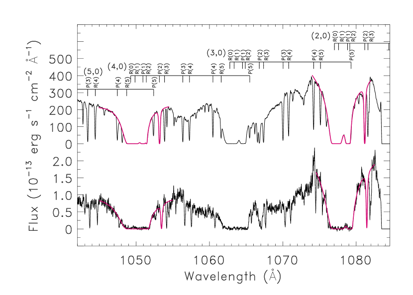
Figure 1: Sample spectra at high and low S/N. Top - HD 210839 (peak S/N $\approx$ 24 per pixel); bottom - HD 154368 (S/N $\approx$ 2). Both spectra have been smoothed to resolution ($\sim$9 pixels) for presentation. This spectral region includes the Lyman series (4,0), (3,0), and (2,0) vibrational bandheads of H₂ (from left to right), as well as broad stellar features at 1057 Å and 1073 Å. A less obvious stellar feature lies near 1067 Å. The numerous narrow lines are mostly due to rotationally excited H₂, as indicated by the series of tickmarks above the spectra; exceptions include Ar I $\lambda\lambda$ 1048,1067 and Fe II $\lambda$1055. Profile fits to the (4,0) and (2,0) bands are shown.

Figure 1 shows sample spectra for a high S/N target (HD 210839) and a low S/N target (HD 154368). The equivalent widths of the undamped $J$ $\geq$ 3 lines can generally be measured individually without regard to the specifics of the unresolved component structure along the line of sight, and then a curve of growth analysis can be performed. We are performing such an analysis, and these results will be presented at a later date. However, to determine the total H₂ column density we must perform profile fits on the highly damped $J$ = 0 and 1 profiles. In addition, since the R(2) lines are blended with the main $J$ = 0 and 1 profiles, we must include $J$ = 2 in the profile fits. Fortunately, the P(2) lines are sufficiently isolated to constrain the $J$ = 2 column densities for our present purposes.

The $J$ = 0 and 1 lines themselves are too heavily damped to be sensitive to the detailed component structure (or $b$-value if a single absorbing cloud is assumed). The $J$ = 2 lines are somewhat sensitive to this choice, and in turn the blending between the P(1) and R(2) lines can affect the derived $J$ = 1 column density. However, we have found that a change in $b$-value of a factor of 2 typically changes log $N$(1) by just 0.01 dex, even with a much greater change in $N$(2).

The steep extinction curves in these heavily reddened lines of sight and the overlap between Lyman and Werner bands of H₂ and the Lyman H I lines prevent us from reliably using H₂ bands near and shortward of Ly$\beta$. Thus, we have considered Lyman bands of H₂ from (0,0) through (4,0).

The continuum radiation from the background hot stars is punctuated by photospheric lines. If these lines lie in the far wings of the damped profiles, they can be easily divided out of the spectra. If they lie near the zero-intensity cores of the profiles, these lines do not affect the overall H₂ spectrum. However, contamination of portions of the H₂ profiles with normalized intensities of $\sim$0.5 is both difficult to remove and can cause significant disruption of the H₂ spectrum. In Paper II we noted that fits of the Lyman (0,0) band in HD 110432 exhibited such contamination, and that the (3,0) band fits were also possibly affected. Further exploration of this issue in additional spectra indicate that contamination of these bands is common. While detailed modeling of the stellar spectra is beyond the scope of this work, we note that the (1,0), (2,0), and (4,0) bands appear to be the cleanest of the long wavelength bands in hot star spectra observed through less H₂. In the interest of producing a uniform measurement of H₂ column densities across our sample, we are limiting our $J$ = 0 and 1 analysis to these bands. These bands appear a total of nine times on five different detector segments.

A final problem is the wide range in data quality. As seen in Table 5, the per-pixel S/N varies from unity to nearly 30. Our data analysis techniques have to work well across this large range.

3.1.2 Fitting techniques

Our goal is to match a model spectrum of the low-$J$ lines to the data by varying the $J$ = 0, 1, and 2 column densities, a quadratic continuum, and a zero-point wavelength shift. We have applied two distinct fitting methods to our data to minimize the squared difference between the model and the data, non-linear least squares (i.e., the Levenburg-Marquardt “CURFIT” algorithm from Bevington & Robinson 1992), and the “downhill simplex method” (the “AMOEBA” algorithm from Press et al. 2000). The non-linear least squares method has the advantage of producing formal uncertainties on each fit parameter from the covariance matrix when using the appropriate weighting scheme. In addition, it is much less computationally intensive. However, this method also requires the evaluation of partial derivatives with respect to each parameter, but our modeled profiles do not have analytical derivatives. The downhill simplex method works to minimize a quantity, in this case the difference between the model and the data, weighted in some manner. The method is more computationally intensive but only requires function evaluations and not derivatives. It can also be much more robust, particularly when dealing with a large number of fit parameters.

We have experimented with several weighting schemes for the data, including “instrumental” (1/error²), “signal-to-noise” (data/error), and “uniform”. Instrumental weighting has the advantage of producing genuine $\chi^{2}$ values and appropriate statistical error bars on each fit parameter, and is the usual choice for astronomical data. However, we have many data sets with very poor data quality (per-pixel S/N of a few or less). In these cases, the generally Poissonian errors can not be reasonably approximated by a normal distribution. This fact tends to skew the weighted fits toward the pixels with smaller values instead of bisecting the data points. Thus, in the poorest quality observations in the present sample, the instrumentally weighted fits do not provide a good match to the data. If we re-bin the data to increase the S/N, this becomes less of a problem. However, such re-binning has its own set of problems. Signal-to-noise weighting is somewhat less susceptible to this problem, although this weighting method is rarely used. A uniformly weighted fit removes this effect completely, but gives limited information on the uncertainties of the fit parameters. In the uniformly weighted fit we are in effect assuming that the perfect model should bisect the data points in a given range for any S/N.

We have tested the various combinations of fitting techniques and weighting schemes. As an example, in Table 6 we show the results of a suite of fits of the (1,0), (2,0), and (4,0) bands from the LiF 1A and LiF 2A segments for HD 199579. This is a high-quality spectrum with S/N of 20 per-pixel at the maxima between the H₂ bandheads, and we would expect to see good agreement among the various methods. The values in Table 6 show that this expectation is verified. Thus, we can choose the fitting technique and weighting scheme most appropriate for our poor-quality data without sacrificing the accuracy of the fits to the good-quality data.

As we observed in Paper II, the largest variation in the fit parameters occurs when comparing one band to another. In addition, the formal uncertainties we derive for the high-quality data sets through both the CURFIT method are less than 0.01 dex. We also performed Monte Carlo simulations whereby we either added noise to synthetic profiles matching the data, or added additional noise to the data itself, and again the changes in the column densities were much smaller than the band-to-band and segment-to-segment differences. From these findings, we confirm our conclusion in Paper II that the largest source of errors in the low-$J$ column densities are from effects other than Poisson noise. These effects include low-level contamination from stellar lines, fixed-pattern noise, wavelength-dependent errors in the flux calibration, and other factors.

3.1.3 Summary of the fitting technique

Based on the previous discussion we now describe our revised fitting technique in full. Before fitting the spectra we identify all visible atomic lines and all visible H₂ lines with $J$ $\geq$ 3, model them with Gaussian profiles, divide the lines out of the spectrum, and exclude from further fitting the cores of the removed lines if they dropped below half of the local continuum level. We also remove obvious stellar lines with a similar procedure. This leaves only seven fit parameters: a quadratic polynomial continuum, logarithmic column densities for $J$ = 0, 1 and 2, and a zero-point wavelength shift. In Paper II, we included the high-$J$ and atomic lines in our fits instead of an outright removal of the lines. Our choice in this matter has little effect on the quality of the fits, but the reduction in fit parameters if we remove the lines reduces the computational time, and tends to make CURFIT as robust as AMOEBA. Also, the number of individual lines that must be modeled is reduced, again reducing the computational time. During the line-removal phase, we also select the appropriate wavelength ranges for the fitting of each band. We make these ranges as uniform as possible from target-to-target and for fits of the same band in different detector segments of the same observation.

We assign a single $b$-value to represent the overall component structure, which only affects the modeling of the $J$ = 2 lines. As stated previously, this value need not be very accurate, and we have used preliminary values from our curve-of-growth analysis of the high-$J$ lines, combined with the high-resolution ground-based data described in § 1.

While there must be unresolved velocity structure in nearly all cases, we do not see evidence for resolved structure in H₂ in any of the 23 targets. The velocity separation we could detect varies from target to target due to S/N issues and differences in strength and saturation level of the high-$J$ lines. However, typical values are 20–30 km s^-1.

We model the line-spread function of the spectrograph with a Gaussian of FWHM corresponding to a resolution, $R$ $\approx$ 17,000. This corresponds to the typical resolution of our spectra which were all observed through the largest available slit (30$\arcsec$ $\times$ 30$\arcsec$). In many cases we are achieving greater resolving power, but even the $J$ = 2 lines are considerably broadened beyond the instrumental profile, and the $J$ = 0 and 1 profiles are not affected by the choice of the line-spread function for any reasonable value.

The H₂ model itself includes the R(0), R(1), P(1), R(2), and P(2) lines of the band being fitted, as well as the R(0), R(1), and P(1) lines of adjacent bands. We must include the latter lines to account for the overlapping damping wings of the $J$ = 0 and 1 lines from adjacent bands. We use line parameters from Abgrall et al. (1993). Once this large model spectrum is calculated on a somewhat finer wavelength grid than the actual spectrum, it is convolved with the line-spread function, the zero-point shift is applied, and the model spectrum is rebinned to the grid of wavelengths from the actual spectrum.

The final fits we report use the CURFIT routine with uniform weighting. In some cases the data quality is too poor at the shorter wavelengths and we can not adequately perform fits of the (4,0) band. Also, the SiC channels have poorer S/N in our range of interest, so in some cases we can obtain fits in the LiF channels but not SiC. A more subtle problem also occurs with the (4,0) band in certain cases. Considerable information is carried by the “bump” between the cores of the R(1) and P(1) lines. This small non-zero section in the spectrum at the saturated core of the vibrational bandheads is very sensitive to the $J$ = 1 column density, and somewhat sensitive to the $N$(1)/$N$(0) ratio, yet it is usually weak enough to be insensitive to issues such as continuum placement. Due to the smaller $f$-values of the lines in the (2,0) and (1,0) bands, the bump is very prominent. But in the (4,0) band, a combination of large column density, poor data quality, and the larger $f$-values can totally eliminate the bump. This situation leaves the fitting routine with only the blue and red wings of the overall $J$ = 0 and 1 profile to constrain the column densities and still accurately define the continuum. In some cases, this leads to unreasonable fits where the continuum will be strongly parabolic instead of relatively flat, and the column density may disagree with other bands by factors of 5–10.

3.2 Error analysis

In the ideal case we have 9 independent measurements of the column densities per observation. (For HD 73882 and HD 206267, the multiple observations give us more measurements.) Since the formal errors on the fits are smaller than the fit-to-fit differences, we adopt the same error analysis as in Paper II, and use as 1-$\sigma$ errors the sample standard deviation of the individual fits. For this choice to be appropriate, the individual fit parameters must be more-or-less normally distributed. We have 16 datasets for which we could obtain all 9 possible column density measurements, and we have used these datasets to search for systematic differences between the individual band/segment combinations. We determined the quantity

$$d=\frac{\log N(J)_{i}-\langle\log N(J)\rangle}{\sigma_{n-1}}$$

for each of the measurements; i.e., the normalized deviation from the line-of-sight mean. If there are no systematic differences, the distribution of $d$ should be normal. Then we found the average of the 16 $d$-values for each band/segment combination, along with the error of the mean.

Table 7 gives the results of this analysis, along with the results for the same band in all segments, and all bands in all segments (whose average must be zero). We immediately see that there are a few systematic differences. The largest difference occurs for the LiF 1A (2,0) $J$ = 0 fits which average nearly 1.5 standard deviations below the overall mean. The red wing of this profile is at the very edge of the detector segment which may affect the continuum determination. There are also relatively large systematic effects in the positive sense for both (1,0) band fits for $J$ = 0, which effectively cancels out LiF 1A (2,0) in the overall average. The source of these effects is consistent with the presence of a very weak stellar line in the blue wing of some of the (1,0) profiles, and an inspection of the fits does suggest that this is the case. In contrast with $J$ = 0, the $J$ = 1 values show much more subtle differences.

Overall, it appears that while systematic differences do indeed occur, they do not have a large effect on the overall results. For example, if we were to exclude the LiF 1A (2,0) fits from the averages, the logarithmic column densities would only change by a few hundredths. We also note that since we have excluded the (3,0) band we do not see band-to-band differences as large as those reported in Paper II. Interestingly, while the cases where we have the fewest individual measurements involve bands with large systematic differences (i.e., LiF 1A (2,0), LiF 1A (4,0), and LiF 2A (1,0)), these systematic effects almost exactly cancel each other out when looking at the ensemble for $J$ = 0, and are small in any case for $J$ = 1. For these reasons, we have included all of these bands in the final averages and uncertainties, i.e. the mean and sample standard deviation of the column densities from the (up to) 9 fits.

4 Results

Table 8 summarizes the measured and derived quantities relating to our H₂ observations, which we will discuss individually in the following sections. We have generally used atomic hydrogen column densities from the literature, derived from IUE observations of the Ly$\alpha$ line. In two cases, we report a new determination of $N$(H I) from our own profile fits of IUE data. For stars later than about spectral type B2, the contribution from the stellar Ly$\alpha$ line becomes large enough to seriously contaminate the interstellar line (§ 2.3.3). Thus, for six lines of sight we have estimated $N$(H I) from the relationship between $E(B-V)$ and $N$(H_tot) (see § 4.2).

Our fundamental observed quantities are $N$($J$=0) and $N$($J$=1), from which we can derive the total molecular hydrogen column density (§ 4.1), total hydrogen column density (§ 4.2), kinetic temperature (§ 4.3), and hydrogen molecular fraction (§ 4.4). In addition, we can assess correlations between H₂ parameters and extinction curve parameters (§ 4.5). The plots in these sections include lines of sight for which $N$(H₂) was measured by Copernicus (Savage et al. 1977). For these targets, we used $N$(H I) from Diplas & Savage 1994 (IUE) and Bohlin et al. 1978 (Copernicus), in order of preference, with most values coming from the former.

4.1 Molecular hydrogen column density

While most of our targets have never been observed at moderate resolution in the far-UV, three targets in our present program were observed by Copernicus, providing measurements of $N$(0) and $N$(1), or at least $N$(H₂). Table 9 compares those values with our new values. The difference for $N$(1) for HD 24534 is quite large, but on the whole the differences are reasonable, given the much larger uncertainties on the Copernicus measurements due to poorer S/N. We also note that we have analyzed several Copernicus targets with our fitting techniques and find very close agreement with the published values.

With the exception of the uncertain measurement of $N$(H₂) toward HD 24534 (X Per) by Mason et al. (1976), which we have refined, all but six of our present H₂ column densities are larger than any observed with Copernicus. In four cases, our column density is larger than the revised value for X Per. We have thus provided the first significant sample of lines of sight with log $N$(H₂) $\approx$ 21.

Figure 2 shows $N$(H₂) as a function of color excess for log $N$(H₂) $>$ 20. Although the column density appears to level off at large color excess, much of this leveling is due to our semi-logarithmic presentation and the linear relationship between total hydrogen column density and color excess described in the following section. Interestingly, most of the scatter in $N$(H₂) for large color excess is due to scatter in $N$(0), as $N$(1) remains nearly constant at 10^20.5 cm^-2. For the 14 FUSE targets with $E(B-V)$ $>$ 0.4, the standard deviation of $N$(0) is 0.21 dex as compared with 0.11 dex for $N$(1), and 0.15 dex for $N$(H₂). This finding is unchanged if we only consider values with uncertainty of 0.1 dex or less. However, it is not clear if this apparent threshold at 10^20.5 cm^-2 is meaningful.

Given our new H₂ measurements, we can extend the range of column densities in exploring correlations with other molecules. In Figure 3 we show the relationships between $N$(H₂) and $N$(CH), $N$(CH⁺), $N$(CN), and $N$(CO). For the Copernicus H₂ targets we took column densities from the compilations of Welty & Hobbs (2001) and Federman et al. (1994) for CH, Allen (1994) for CH⁺, and Federman et al. (1994) again for CN and CO. We have only included absorption measurements since that step gives the best guarantee that we are sampling the same material as in the H₂ measurements.

The excellent relationship between CH and H₂ seen in previous investigations continues to be reflected when adding our new data. The relationship is nearly linear, in agreement with Danks, Federman, & Lambert (1984). Chemical models predict a linear relationship between $N$(CH) and $N$(H₂), with some scatter due to variations in density (Danks et al. 1984; van Dishoeck & Black 1988, 1989).

We also find a linear relationship between CH⁺ and H₂, with some outlying points and considerable scatter. The primary formation reaction for CH⁺ is endothermic, and thus shocks have been proposed as an energy source for the reaction (Elitzur & Watson 1978). Lambert & Danks (1986) found a good correlation between “warm” gas as measured by the rotational excitation of H₂ for $J$=3–5, and $N$(CH⁺), supporting the shock hypothesis. Our future measurements of rotationally excited H₂ may shed additional light on this issue.

Allen (1994) previously found that log $N$(CH⁺) increases with $E(B-V)$ up to about 0.6, then levels off. However, this primarily occurs due to the semi-logarithmic axes and this relationship actually remains more or less linear up through $E(B-V)$ = 1.2. Gredel (1997) also found linear relationships between $N$(CH⁺) and extinction ($A_{V}$) within individual OB associations. In addition, Gredel found a correlation between $N$(CH⁺) and $N$(CH). Gredel concluded that the dissipation of turbulence may be an important production mechanism.

Another statistically significant relationship appears between CN and H₂, similar to that found by Danks et al. (1984). The CN radical is highly density sensitive in the range of column densities studied here (Federman, Danks, & Lambert 1984). We also see a strong correlation between CN and molecular fraction (§ 4.2), and we would expect the latter quantity to also be correlated with density. The chemical models of van Dishoeck & Black (1988, 1989) appear to trace only the upper envelope of the observed CN abundances, but this model is for $n$ $\sim$ 500 cm^-3. Low- and high-density models of Federman et al. (1984) appear to bracket our new data as they did for the Federman et al. dataset.

Finally, we see that CO and H₂ are also highly correlated. The slope of the relationship appears to become more gradual at the highest column densities. At log $N$(H₂) $\sim$ 20.5, the CO column density begins to increase more rapidly than H₂. However, this is also the point where saturation effects become very important in assessing $N$(CO) and in several cases a small $b$-value ($\sim$1 km s^-1) has been assumed which may not be appropriate if multiple components exist. Even a modest increase in the $b$-value can result in a decrease in column density of an order of magnitude if the line lies on the flat part of the curve of growth.

On the other hand, chemical models do predict a rapid increase in CO column density relative to $N$(H₂) within the range of column densities studied in the present work. The models from van Dishoeck & Black (1988, 1989) show good agreement with the limited data. Absorption-line measurements of CO are difficult within the FUSE bandpass as the rotational structure is poorly resolved and the lines are often saturated. HST observations of the A–X series of CO lines will be crucial for extending the CO/H₂ ratio.

We note that while the correlations between the line-of-sight quantities are generally strong, some caution is necessary. As we discuss in § 5.2, we can not assess the true distribution of the majority of the H₂ along the line of sight. Thus, in cases where the various molecules are distributed across a range of velocities, the line-of-sight correlations may not be physically meaningful. In particular, the column density of CN is sensitive to particle density and is expected to only trace the densest cloud cores.

4.2 Total hydrogen column density

First, we can look at the relationship between the total hydrogen column density, $N$(H_tot) = 2$N$(H₂) + $N$(H I), and color excess; i.e., the gas-to-dust ratio. Bohlin et al. (1978) found a linear relationship from Copernicus data, $N$(H_tot) = (5.8 $\times$ 10²¹ cm^-2) mag^-1 $E(B-V)$. In Figure 4, we have plotted the Copernicus/IUE dataset, along with our present FUSE sample. The new data fit the old relationship remarkably well, and the FUSE data alone give a slope of 5.6 $\times$ 10²¹ cm^-2 mag^-1. There are a few disagreements larger than the error bars, but the largest deviation for $E(B-V)$ $>$ 0.3 is for the Copernicus/IUE observations of $\rho$ Oph A ($E(B-V)$ = 0.47, log $N$(H I) = 21.7). This deviation still occurs with the revised IUE H I measurement (Diplas & Savage 1994) even though it represents a significant downward revision of the original Copernicus value.

This enhanced gas-to-dust ratio for $\rho$ Oph A has been interpreted as due to a preponderance of large grains within the $\rho$ Oph cloud (Bohlin et al. 1978). These large grains are less efficient at producing visual reddening, and thus the $E(B-V)$ color excess underestimates the actual quantity of dust. The unusual dust properties also lead to an unusual extinction curve and a very large value of $R_{V}$. We note that we have only a single line of sight in our present sample with $R_{V}$ $>$ 4 (HD 102065) and we do not have an independent measurement of $N$(H I) for this target.

4.3 Kinetic temperature

In deriving the temperature of the gas, $T_{01}$, we assume that the density and column density are high enough such that thermal proton collisions dominate over other processes in determining the ratio $N$(1)/$N$(0), and that the observed populations obey the Boltzmann relation. In textual form, we will refer to this temperature as the “kinetic temperature”, while symbolically we will use $T_{01}$ to emphasize the source of this temperature. In addition, we emphasize that this temperature is a “column-averaged” temperature, while the actual temperature will vary throughout the cloud(s) in the line of sight.

With a ratio of statistical weights, $g_{1}$/$g_{0}$ = 9, the population ratio is simply

$$\frac{N(1)}{N(0)}=9e^{-E_{01}/kT_{01}},$$ (8)

where $E_{01}$/$k$ = 171 K. With column densities expressed as base-10 logarithms (as in Table 8), the kinetic temperature (in K) can then be written

$$T_{01}=\frac{74}{\log N(0)-\log N(1)+0.954}.$$ (9)

In calculating the uncertainties in kinetic temperature, we take the combination of 1-$\sigma$ errors that gives the largest deviation from the best value, such that the errors on the derived values are more conservative. Furthermore, in deriving these errors, we have taken 0.04 dex as the minimum possible error on a column density, even when we have derived a smaller error. This corresponds to 10% and while this choice is arbitrary we feel that it is a reasonable guess for the magnitude of any systematic effects.

The average kinetic temperature derived from Copernicus observations of 61 lines of sight with log $N$(H₂) $>$ 18.0 was 77 $\pm$ 17 K (Savage et al. 1977). A similar calculation for the 9 Copernicus lines of sight with log $N$(H₂) $>$ 20.4, comparable to the present survey, gives 55 $\pm$ 8 K. Our FUSE sample gives an intermediate value, 68 $\pm$ 15 K. However, we note that our sample has a somewhat unusual distribution, with three lines of sight having $T_{01}$ $\geq$ 94 K, but none in the range 75–93 K. In any case, our average value is similar to that found previously for lines of sight where H₂ is self-shielded.

Despite extending the range of color excess by a factor of 2, Figure 5 shows that the kinetic temperature in our sample does not change with increasing $E(B-V)$. We have also searched for a correlation between $T_{01}$ and $R_{V}$ and found none. We might expect the kinetic temperature to be anti-correlated with density indicators, and we see such a relationship between $T_{01}$ and $N$(CN) (Figure 6). The slope of the relationship is quite small and there are a few outlying points, but given the small range in the observed temperatures, the relationship is quite good.

4.4 Molecular fraction

The hydrogen molecular fraction, $f_{\rm H2}$, gives the fraction of hydrogen atoms in molecular form. In terms of the column densities of H I and H₂,

$${f_{\rm H2}}=\frac{2N(H_{2})}{2N(H_{2})+N(HI)}$$ (10)

The tabulated uncertainties for molecular fraction follow the same procedure described in the previous section.

The Copernicus data showed an interesting trend of molecular fraction with increasing color excess (Savage et al. 1977). Below $E(B-V)\approx 0.08$, the molecular fraction is quite small, typically less than 10^-4, while above this point the fraction is generally greater than 10^-2, with few points lying in between. This abrupt boundary occurs due to increased self-shielding of H₂ near $N$(H₂) $\sim$ 10¹⁶ cm^-2, corresponding to $f_{\rm H2}$ $\sim$ 10^-5.

In Figure 7, we show molecular fraction versus color excess for the Copernicus data and our FUSE data. The boundary at $E(B-V)\approx 0.08$ is not visible because we have chosen a linear scale for the ordinate. The FUSE data mostly overlap values found previously, but we have greatly increased the number of lines of sight with at least moderately high molecular fraction. Even in the range of overlap of the two samples, the FUSE sample shows larger molecular fractions, but this is probably a selection effect. We do not see an increase in molecular fraction with increasing extinction within the FUSE sample.

Figure 8 shows the molecular fraction versus the total-to-selective extinction ratio, $R_{V}$, for the FUSE dataset. Previous results have suggested an anti-correlation between the two quantities for diffuse clouds, consistent with idea that grain coagulation reduces the available surface area for H₂ formation at larger $R_{V}$ (Cardelli 1988). However, our data do not show a statistically significant relationship between the two quantities. We do not presently have good coverage of large values of $R_{V}$, but several lines of sight with $R_{V}$ $>$ 4 remain to be observed as part of the FUSE translucent cloud program.

Although little-mentioned, the Copernicus data show a good correlation between molecular fraction and kinetic temperature. Figure 9 shows both data sets, and while the FUSE data themselves show only a weak relationship, those points still follow the general trend. There are lines of sight with small molecular fraction at all kinetic temperatures, but lines of sight with large molecular fraction are preferentially associated with small kinetic temperature. This relationship is not surprising as both large molecular fraction and small kinetic temperature should be associated with denser cloud cores. In a similar sense, we also see a correlation between molecular fraction and the density-sensitive CN abundance (Figure 10).

4.5 Extinction curve parameters

With six extinction curve parameters and four column-density related quantities ($f_{\rm H2}$, $N$(CH)/$N$(H_tot), $N$(CH⁺)/$N$(H_tot), $N$(CN)/$N$(H_tot)), we have 24 potential correlations. In addition to our FUSE data points, we have included the handful of points from the Fitzpatrick & Massa (1986, 1988, 1990) and Jenniskens & Greenburg (1993) extinction curve surveys for which we have the ancillary data. We have evaluated the Spearman rank correlation coefficient for each of these relationships. In 11 cases the correlation is not significant at the 1$\sigma$ level, while 10 correlations are significant at the 2$\sigma$ level. Thus, we generally either find no correlation or a good correlation in the statistical sense. The 2$\sigma$ group includes $N$(CN)/$N$(H_tot)) vs. both $c_{1}$ and $c_{2}$; $N$(CH⁺)/$N$(H_tot) vs. $c_{3}$; $f_{\rm H2}$, $N$(CH)/$N$(H_tot), and $N$(CN)/$N$(H_tot)) vs. both $c_{4}$ and $\gamma$; and $N$(CH)/$N$(H_tot) vs. $\lambda_{0}^{-1}$. Since the main focus of this paper is H₂, we will consider the two strong correlations involving $f_{\rm H2}$ in detail.

The strongest (3.7$\sigma$) and most intriguing correlation is that between molecular fraction and the width of the 2175 Å bump, $\gamma$ (Figure 11). In fact, of all the parameters we have considered in the present work, $\gamma$ appears to be the best predictor of molecular fraction. The larger molecular fractions appear to be associated with regions of larger density. Thus, our findings suggest that the width of the 2175 Å bump is closely related to density. Fitzpatrick & Massa (1986) reported a similar finding in a qualitative sense; dense quiescent regions such as dark clouds and reflection nebulae were associated with broad bumps, and diffuse clouds and star-forming regions were associated with narrower bumps. They found a good correlation between $\gamma$ and $E(B-V)$/$r$, where $r$ is the distance to the star, even with the biases associated with this density indicator. Our observed correlation between $f_{\rm H2}$ and $\gamma$ shows much less scatter and could well be taken as linear. The single outlying point, $\zeta$ Oph, showed the largest difference in $\gamma$ between the two methods used by Fitzpatrick & Massa (1986, 1990). We have used the final value of Fitzpatrick & Massa (1990) based on the overall extinction curve fits, but the initial value, based on just the region around the bump, would lie much closer to the rest of the points. The authors attributed this large difference to the relative shallowness of the bump and the resultant uncertainty in separating the bump from the rest of the extinction curve.

Ignoring $\zeta$ Oph, an unweighted linear fit of the rest of the points gives the relation,

$$f_{\rm H2}=1.44\gamma-1.04$$ (11)

corresponding to a minimum value of $\gamma$ of 0.72, and a maximum value of 1.42. (If we include $\zeta$ Oph in the fit, the allowed range is 0.67–1.51.) In fact, the extrema in $\gamma$ in the entire Fitzpatrick & Massa (1990) and Jenniskens & Greenberg (1993) samples of more than 100 curves are 0.76 and 1.383 (or 1.25 if we ignore $\zeta$ Oph).

While the bump width appears to be a good predictor of molecular fraction in our sample, this relationship may not hold in all environments. For example, many lines of sight in the SMC have no discernible 2175 Å bump at all (Gordon & Clayton 1998). On the other hand, in a survey of 30 Galactic lines of sight selected to sample low-density gas, Clayton, Gordon, & Wolff (2000) found small values of $\gamma$ ($\lesssim$1.0). This finding is consistent with the likelihood that the lines of sight sample gas with low molecular content. Thus, a strong correlation between molecular fraction and bump width may apply in most Galactic environments, albeit the relationship may not be linear.

The strength of the far-UV curvature, $c_{4}$, exhibits the other strong correlation with $f_{\rm H2}$, at the 2.6$\sigma$ level (Figure 12). The extrema in $c_{4}$ are HD 102065 and HD 62542, and these points show up as outliers in the relationship. Although neither line of sight has a well-determined value of $f_{\rm H2}$ it is highly unlikely that our reported values are so inaccurate as to match the apparently linear trend with $c_{4}$ seen in the other points. The presence of this correlation is consistent with the previously noted tendency for a steep far-UV rise to be associated with a broad 2175 Å and the observed correlation between the bump width and molecular fraction.

An alternative explanation for the correlations between molecular fraction and both the bump width and far-UV curvature concerns the properties of the dust grains. Increased far-UV curvature is thought to be associated with smaller than normal dust grains (Cardelli, Clayton, & Mathias 1989). The 2175 Å bump is most likely associated with small carbonaceous grains (Désert, Boulanger, & Puget 1990), and perhaps smaller grains lead to broader bumps.

Grain size is also thought to be smaller in lines of sight with small $R_{V}$, and Cardelli (1988) found an inverse correlation between molecular abundances and $R_{V}$. He attributed this correlation to the effects of these smaller grains and their effect on H₂ formation and destruction. With similar total grain masses, the smaller grains will provide greater surface area, yielding a greater H₂ formation rate, and a smaller photodissociation rate via the increased far-UV extinction. We recall, however, that in the present work, we do not find a good correlation between molecular fraction and $R_{V}$.

5 Discussion

In this section, we will mainly focus on what our findings say about the nature of our present lines of sight relative to diffuse clouds. The overall line-of-sight characteristics of most of our present sample satisfy the criterion to be considered “translucent”, i.e. $A_{V}$ $\gtrsim$ 1. Implicit in the definition of a translucent cloud is that we are considering a single molecular cloud, and not a collection of several diffuse clouds. For the purposes of this discussion, we adopt a definition of a “translucent cloud” similar to that envisioned by van Dishoeck & Black (1988); i.e. $f_{\rm H2}$ $\gtrsim$ 0.9, $T_{01}$ $\lesssim$ 40 K, and $A_{V}$ $\gtrsim$ 1. Such a cloud may be an isolated cloud, a skin around a dense cloud, or a core located within significant diffuse material.

If a line of sight is dominated by one of these clouds, we would expect this situation to be reflected in several of our measured quantities. Specifically, the observed molecular fraction should be large, while the kinetic temperature should be small. As shown in Figure 9, these two quantities do indeed show an anti-correlation, with considerable scatter. Despite the scatter, all of the lines of sight where $N$(H₂) $>$ $N$(H I) ($f_{\rm H2}$ $>$ 2/3) show small kinetic temperatures. In fact, there appears to be a distinct group of 10 lines of sight centered near $T_{01}$ = 55 K and $f_{\rm H2}$=0.7 that is separated from the rest of the sample. This is even more apparent if we ignore the FUSE data points without direct measurements of $N$(H I).

However, there are several lines of sight with similar or even smaller kinetic temperatures than this group of 10. In addition, while the molecular fractions are relatively large, they do not closely approach unity as we might expect. Also, the extinctions for several of these lines of sight are less than or equal to one magnitude, barely satisfying the rather loose definition of a translucent cloud we have adopted. To further assess the question of whether we are seeing individual translucent clouds, we need to consider the distribution of material along the line of sight (§ 5.1). We also consider evidence from studies of chemical depletions (§ 5.2). Finally, we consider the question of why we see few, if any, translucent clouds in our lines of sight (§ 5.3).

5.1 Multiple clouds and “hidden” translucent clouds

Arguing in favor of the hypothesis that we are seeing at least a few translucent clouds is the fact that the overall line-of-sight column densities can be greatly affected by the particular distribution of material. Even if highly molecular material exists, there could be a skin of diffuse material surrounding this cloud, or additional diffuse clouds along the line of sight. In these cases, the observed integrated molecular fraction could be considerably less than unity and the kinetic temperature could be affected as well. Thus, even a line of sight with only a moderately high molecular fraction could harbor a translucent cloud.

Chemical modeling of the lines of sight can, in principle, help constrain the distribution of material. Models have been constructed which reproduce the column densities of a variety of species in diffuse clouds, including H₂ (e.g., van Dishoeck & Black 1986). In some lines of sight, the models have difficulty reproducing the high-$J$ column densities of H₂ (e.g., Paper II).

Part of our group has developed a new code to study the formation, destruction, radiative transfer, and ro-vibrational excitation of H₂ (Browning et al. 2002). Several lines of sight with published high-$J$ column densities for H₂ have been modeled with this code, including HD 110432 and HD 73882. In many cases, it was difficult to model a line of sight as a single cloud without invoking extreme conditions, such as a radiation field 10–100 times the Galactic mean, which is unrealistic in most cases. Better matches require multiple clouds and/or multiple pathways for incoming UV radiation. In addition, changes in one physical parameter can mask changes in another such that a group of models corresponding to a range of physical conditions will all match the column densities for an individual line of sight. Ensembles of models, combined with large samples of lines of sight, can provide more definitive results, such as in the LMC/SMC (Tumlinson et al. 2002).

We can also observationally study the possibility that the H₂ along these lines of sight lies in several distinct clouds, with corresponding smaller extinctions for each cloud. The very high resolution ground-based data show that most lines of sight have numerous components in Na I and K I, and the strongest components usually lie within a 10 km s^-1 velocity range (D. E. Welty et al. 2002, in preparation). Data for the CH radical show similar behavior. Given the good correlations between $N$(H₂) and these species, we might expect the H₂ to also be distributed among several components.

We can assess the distribution of H₂ indirectly, in several ways. Equivalent width data allow us to perform a curve-of-growth analysis of the high-$J$ lines. Most simply, we can construct a best-fit single-component curve of growth via fitting techniques and determine the best values for the column densities of each $J$-level as well as the optimum “effective” $b$-value of the distribution. However, we can not always assume that the actual component structure is well approximated by a single $b$-value. Our program of high-resolution spectroscopy allows us to better constrain the component structure with the assumption that some or all of the components seen in Na I and/or K I and/or CH contain H₂, with perhaps a scaling of the $b$-values of the individual components, and possible variation in the ratios of the ground-based species to H₂ from component to component. As we have seen, for the overall lines of sight, there is a nearly one-to-one correspondence between CH and H₂, and strong correlations also appear for Na I and K I (Welty & Hobbs 2001).

In our preliminary investigations of the high-$J$ H₂ lines, we often find a better match with “effective” $b$-values greater than can be obtained with the CH component structure. We would then have to use additional components observed in K I or Na I — including some of the weaker components, as compared with only using the strongest. Thus, even with a “simple” component structure, the H₂ still appears to be distributed among several closely-spaced velocity components. Despite the small separations, the components are resolved in the very high resolution optical spectra, which suggests discrete components and not just material more-or-less uniformly distributed in velocity space. With the additional components that may contribute at least small amounts of H₂ to the overall observed column densities, the quantity of H₂ available in each component is further diluted.

One important caveat to this discussion of the component structure is that in looking at the high-$J$ lines we are considering only 1% or less of the total H₂. We have little hope of directly assessing the true component structure of the extremely strong $J$ = 0–1 lines. In addition, the $J$ = 2 lines are also very strong and heavily saturated or even damped, and will not always provide constraints to the component structure. We expect the material containing the low-$J$ lines to mostly be located in the self-shielded cloud core(s), while the material containing the high-$J$ lines may be more physically widespread along the line of sight. Thus, the component structure corresponding to $J$ = 0 and 1 may be simpler than that for the high-$J$ lines.

There is a tendency for the lines of sight with the largest molecular fractions to have the simplest component structures when looking at CH or the strong Na I and K I components that are most likely to also contain H₂ (D. E. Welty et al. 2002, in preparation). In Table 10 we give preliminary information on the CH component structures observed at high resolution. We caution that the 4 cases with a single component are for observations at the lowest resolutions. The typical spacing between components is 3–5 km s^-1, so there may be unresolved structure, as indicated in higher resolution K I spectra in these 4 cases. In fact, we find more complex structure in the K I spectra in all lines of sight in Table 10. It is more difficult to detect weak components or resolve closely spaced components in CH observations due to $\Lambda$-doubling, the small atomic weight, and the relatively weak spectral lines. In the CH data with resolution of less than 2 km s^-1, the lines of sight with more material in the strongest component and/or fewer components have larger molecular fractions. These lines of sight presumably have less contamination from foreground clouds of atomic gas. Yet, in all cases where we have this “very high” resolution data, there are multiple components, with no more than $\sim$75% of the molecules in the dominant component.

Given the relatively close spacing of the CH components we have to consider whether they represent small knots of material within a single cloud, or distinct clouds along the line of sight. If we are dealing with knots of material within a single cloud, we still might consider this cloud to be a translucent cloud due to the large overall extinction and high molecular content. Also, within a single cloud, the extreme widths of the H₂ $J$ = 0 and 1 lines effectively self-shield the entire range of velocities. If we are dealing with multiple distinct clouds at the even closer spacing suggested by the K I data, the amount of molecular material within the most abundant cloud core will generally be even less than indicated in Table 10 (or in our mathematical analysis below and in Table 11). This suggests that these lines of sight are simply collections of many diffuse clouds with small extinction, albeit with large molecular fractions and presumably relatively high densities.

An indirect method for assessing the quantity of H₂ and H I in each component comes from the study of chlorine. The chemistry of chlorine is intimately connected to that of H₂ because of the large reaction rate with Cl II. With a first ionization potential of 13.01 eV, chlorine will be primarily ionized in H I gas, and primarily neutral in association with H₂ (Jura 1974; Jura & York 1978). Thus, observations of Cl I and Cl II lines (in the UV) can constrain the hydrogen molecular fraction. P. Sonnetrucker et al. (2002, in preparation) have used this technique to infer that the true molecular fraction in the dominant area of H₂ toward HD 192639 is as large as twice the line-of-sight value (2/3 vs. 1/3). High-resolution measurements of the the Cl I $\lambda$1347 line may provide important constraints on the molecular fractions of individual velocity components toward our lines of sight.

While detailed physical and chemical modeling of these lines of sight will appear in a later paper or papers, we can perform a feasibility analysis on the H₂ column densities in each line of sight to assess the possible presence of translucent clouds. I.e., we know the overall line of sight parameters, and we also know approximately what a translucent cloud should look like. Thus, we can add the expected observed properties of putative translucent clouds to diffuse cloud material in various combinations that produce the observed total line of sight quantities. While not a physical model of the clouds, it does provide interesting constraints on the observable quantities.

We define translucent material as having $f_{\rm H2}$ = 0.9 and $T_{01}$ = 30 K, comparable to the parameters used in the translucent cloud models of van Dishoeck & Black (1988). To constrain the total column density of the translucent cloud and the remaining material, we assume that the previously discussed relationship between $E(B-V)$ and $N$(H_tot) still applies for highly molecular clouds. We then mathematically create the largest embedded translucent cloud that is still consistent with the line of sight totals, and that produces realistic parameters for the remaining “diffuse” material, i.e. $T_{01}$ $<$ 200 K. If the line of sight molecular fraction is small and the temperature is large, only a small amount of material could possibly be locked up in a cold, highly molecular cloud, and vice versa.

In Table 11 we give our results for this breakdown of material into translucent and diffuse clouds. From this simulation, we see little evidence for individual translucent clouds along our lines of sight. In two directions, HD 73882 and HD 154368, translucent clouds with $A_{V}$ $\sim$ 1 could exist. The remaining diffuse material still has a molecular fraction appropriate for the color excess. HD 62542 is the only direction where more than half of the material could be translucent.

If we were to relax the criteria for a “translucent” cloud to something like $f_{\rm H2}$ = 0.8 and $T_{01}$ = 40 K, comparable to the most extreme line of sight values we actually see, we would then have many more cases where there is as much translucent material as diffuse. Not coincidentally, this larger list of lines of sight with as least as much translucent material as diffuse is identical to the list of FUSE targets in the upper left-hand portion of Figure 9 discussed at the beginning of § 5. However, we would still not have additional translucent clouds with $A_{V}$ $>$ 1.

We have assumed a gas-to-dust ratio of 5.8 $\times$ 10²¹ cm ^-2 mag^-1 based on the excellent match we see in Figure 4. The observed scatter could support variations on either side of this relationship for our FUSE targets, albeit not as large as seen for $\rho$ Oph. However, we would need large (and unrealistic) differences in the dust characteristics between the “diffuse” and “translucent” material to modify our conclusions in the previous paragraphs.

5.2 Evidence from chemical depletions

As noted in § 2.3.13, chemical depletions can be used as an indicator of the presence of translucent clouds. For HD 192639, the depletions of about a dozen species indicate similar conditions to diffuse clouds (P. Sonnentrucker et al. 2002, in preparation). We have also undertaken a study of Fe II depletions in most of our FUSE targets (Snow, Rachford, & Figoski 2002). Snow et al. found that the depletion of iron is more or less uniform for the FUSE lines of sight. There is little evidence for increased depletion with increasing extinction, molecular fraction, or $N$(H_tot)/$r$, within the range of $E(B-V)$ and $A_{V}$ covered by FUSE. The new observations did not extend the trends of increasing depletion with increasing density found by Savage & Bohlin (1979) and Jenkins, Savage, & Spitzer (1986). Such increased depletions are expected to occur at some point within the translucent clouds (Snow et al. 1998). Given the moderate resolution of the FUSE Fe II observations, we can not rule out the possibility of large depletions for individual components, which become “smoothed out” in the line-of-sight values.

Two of our FUSE targets with particularly large molecular fraction, HD 24534 and HD 154368, have been observed at high resolution with HST to search for increased depletions in several additional species. The results for HD 24534 show a very slight, and probably not statistically significant, increase in carbon depletion relative to diffuse clouds (Sofia, Fitzpatrick, & Meyer 1998). Snow et al. (1998) did not find increased oxygen depletion toward HD 24534. Snow et al. (1996) studied many species toward HD 154368 and also did not find increased depletions. They concluded that the line of sight toward HD 154368 contained extended regions of moderate-density gas instead of one or more dense cloud cores, despite $A_{V}$ $\approx$ 2.5.

5.3 Where are the translucent clouds?

While each of techniques we have discussed has limitations, we are forced to conclude that with few exceptions there is little evidence for individual translucent clouds within our lines of sight, based on the definition given at the beginning of this section. For HD 24534, HD 154368, and HD 192639 we have considerable information that leads to this conclusion, while the evidence for the rest of the lines of sight is more circumstantial. There are several possible reasons why we have not found such clouds:

1. Translucent clouds are just beyond our FUSE range.
Very few stars have enough UV flux to be observed with FUSE through $A_{V}$ $>$ 2, and our present sample includes only seven such targets. Many interesting targets were rejected from the original potential target list for being too faint. Several of these targets have $A_{V}$ = 2–4 (e.g. HD 80077, HD 169454) and lie behind molecular clouds. When combined with the fact that many, if not most, lines of sight will have contaminating diffuse material, we may need to reach $A_{V}$ $\sim$ 3–5 to find evidence for individual clouds with molecular fractions near unity and $A_{V}$ $\sim$ 1–2.

Chemical models suggest that several important transitions involving carbon take place in clouds in the range $A_{V}$ $\sim$ 1–3, such as increased CO abundance and a dramatically larger C I/C II ratio (e.g., van Dishoeck & Black 1988, 1989). There is also evidence for changes in grain conditions at $A_{V}$ $\sim$ 3. For example, Whittet et al. (2001) find an increase in $R_{V}$ in the Taurus dark clouds for $A_{V}$ $>$ 3. The 3-$\mu$m water-ice feature begins to appear at this point as well, lending support for the idea that grain mantle growth becomes important here.

2. $\zeta$ Oph-type lines of sight are indeed “translucent.”
As we have mentioned, large molecular fractions do seem to be correlated with not only simpler component structures, but also low kinetic temperatures, large column densities of density-sensitive species such as CN, and the environment-sensitive 2175 Å bump width and far-UV extinction curvature. If we were to relax the requirement for large $A_{V}$, we could consider all 10 lines of sight discussed in the preamble to this section as containing “translucent clouds.” However, we note that even within this group, the already small $A_{V}$ is sometimes broken up into even smaller clouds (such as toward $\zeta$ Oph). We are reluctant to accept this possibility without a confirmation that we do not see large molecular fractions in appropriate targets with large $A_{V}$.

3. There is no distinction between “diffuse” and “translucent” except larger $A_{V}$.
This possibility is the simplest. However, there is significant evidence listed above to support the idea of at least a gradual transition in physical parameters through $A_{V}$ = 1–5, if not more abrupt transitions. Again, we feel that we need to cover a larger range of $A_{V}$ before we could accept this possibility.

We feel that the first possibility is the most likely one based on our present findings. The ubiquity of interstellar clouds makes it difficult to find lines of sight that only sample a single cloud, or stars that are still observable through an ensemble of several clouds that might contain a translucent cloud.

A more definitive answer to the question posed in this section would require H₂ observations of several lines of sight with $A_{V}$ $>$ 2 where the neutral atoms and simple carbon-containing molecules show relatively simple velocity structure such as HD 169454 (Jannuzi et al. 1988; Crawford 1997). Even in this case, the Na I component structure is more complicated (Federman & Lambert 1992). A more serious problem is that FUSE is barely capable of this observation, and is incapable of observing several other promising targets such as HD 80077. We note that while the decrease in observed UV flux due to increasing H₂ absorption plays a role in limiting the number of targets we can access, it is a very small role. For instance, we can calculate model H₂ absorption spectra and compare the height of the peaks between the vibrational bandheads for N(H₂) = 1 $\times$ 10²¹ (present sample) and 5 $\times$ 10²¹ cm^-2 (a highly molecular cloud with $A_{V}$ $\approx$ 5–6). For this extreme example, the intensity relative to the continuum at the peaks on either side of the (4,0) bandhead is $\approx$0.85 for the low-column case, and $\approx$0.45 for the high-column cases. However, the effect at the (2,0) and (1,0) bandheads is much smaller since these bands are weaker, i.e., $\approx$0.95 versus $\approx$0.75. This is a trivial effect relative to the increased dust extinction, and indicates that our dataset is not significantly biased against high-column lines of sight through selection effects.

As a final note, we emphasize that there is a subset of lines of sight with relatively small extinction, but extreme line of sight characteristics. These include HD 62542 and HD 210121, both of which appear to have a large molecular fraction, and are among the best candidates for having translucent clouds based on Table 10. We may eventually find lines of sight with larger $A_{V}$ that indeed contain individual clouds similar to those toward HD 62542 and HD 210121 and thus the latter would be considered translucent clouds.

6 Summary

We have completed the first FUSE survey of molecular hydrogen in lines of sight with $A_{V}$ $\gtrsim$ 1. The survey includes observations toward 23 early-type stars, which sample gas in a range of environments. Through profile fitting of three vibrational bandheads, we have directly measured the H₂ column densities in the $J$ = 0 and $J$ = 1 states. Combined with ancillary data, we have then derived the total H₂ column density, hydrogen molecular fraction, and kinetic temperature. In addition, we have compiled a set of extinction parameters for our lines of sight.

With this information we have investigated many important relationships between parameters. We have extended previous correlations between $N$(H₂) and $N$(CH), $N$(CH⁺), $N$(CN), and $N$(CO). While the formation of CH⁺ is still an open question, the other correlations closely match predictions from chemical models, despite possible differences in the distribution of these species. We find a potentially powerful combination in assessing the H₂ content of a line of sight based on ground-based measurements and IUE or HST mid-UV observations. The excellent relationship between $N$(H₂) and $N$(CH) gives a good estimate of $N$(H₂), while the measurement of the width of the 2175 Å bump gives a good estimate of molecular fraction.

We find a generally self-consistent picture of these lines of sight in the sense that various indicators of density correlate well with each other; i.e., molecular fraction, kinetic temperature, CN abundance, and extinction curve parameters.

While our sample has a relatively large average molecular fraction, we have not found lines of sight with molecular fractions greater than 0.8. We have identified a subset of 7 lines of sight (plus 3 lines of sight observed by Copernicus) with large molecular fraction and small kinetic temperature which represent the best candidates for the presence of “translucent cloud” material. However, the possible quantities of material that could be associated with translucent clouds generally corresponds to $A_{V}$ $<$ 1 mag, the nominal lower limit for such clouds, and in no case do we see evidence for highly molecular material corresponding to $A_{V}$ $\gtrsim$ 1.5 mag. In addition, in most cases we see evidence for multiple velocity components for H₂, which would further divide up the extinction when considering the individual clouds. Thus, our conclusion is that for the present sample we are observing only a few individual translucent clouds. Rather, we are mostly seeing combinations of diffuse clouds. We suggest that without specific evidence to indicate individual translucent clouds, lines of sight with $A_{V}$ $\gtrsim$ 1 should be called “translucent lines of sight” and the term “translucent cloud” should be avoided.

An ongoing analysis of the high-$J$ lines of H₂ in these lines of sight, combined with a detailed modeling program similar to that for the Magellanic Clouds (Tumlinson et al. 2002), will allow us to better assess the physical conditions in the clouds. This will be the first large study of high-$J$ excitation of H₂ to incorporate very high resolution ground-based observations of species such as K I, Na I, and CH to help assess the unresolved component structure of H₂. Also, we are undertaking detailed analysis of all available species in selected individual lines of sight (e.g. P. Sonnentrucker, et al. 2002, in preparation, for HD 192639), combining FUSE data with recently obtained HST data. Further studies with HST in the lines of sight with the largest molecular fractions will also be useful.

Finally, several additional lines of sight from the FUSE translucent cloud survey have already been observed since the cut-off date for inclusion in the present work (June 2001), and we anticipate that most of the 21 remaining targets will be observed. Several very important targets such as HD 37903 and HD 147889 are part of the program. These additional observations will double the number of lines of sight studied, and should improve and/or extend the results of the present work.

Figure 2: Molecular hydrogen column density vs. color excess. Symbols - crosses: FUSE; diamonds: Copernicus

Figure 3: H₂ column density vs. other molecular column densities. Symbols as in Figure 2. Solid curves in panels a), b), and d) are translucent cloud models from van Dishoeck & Black (1989). Dotted lines in the bottom right corner of each panel correspond to unit slope for that panel.

Figure 4: Symbols as in Fig. 2. The six FUSE points with no independent measurement of $N$(H I) are not included. The solid line corresponds to the relation $N$(H_tot) = (5.8 $\times$ 10²¹ cm^-2 mag^-1)$E(B-V)$ given by Bohlin et al. (1978).

Figure 5: Kinetic temperature vs. color excess. Symbols - crosses: FUSE; diamonds: Copernicus points with $N$(H₂) $>$ 10²⁰ cm^-2; squares: Copernicus points with $N$(H₂) $<$ 10²⁰ cm^-2.

Figure 6: Kinetic temperature vs. fractional CN abundance. Symbols as in Figure 5. (Note the particularly large error bar for BD $+$31^∘ 643 on this expanded vertical scale.)

Figure 7: Molecular fraction vs. color excess. Symbols - crosses: FUSE; asterisks: FUSE points with no independent measurement of N(H I); diamonds: Copernicus points with $N$(H₂) $>$ 10²⁰ cm^-2; squares: Copernicus points with $N$(H₂) $<$ 10²⁰ cm^-2.

Figure 8: Molecular fraction vs. total-to-selective extinction. Symbols as in Figure 5.

Figure 9: Molecular fraction vs. kinetic temperature. Symbols as in Figure 7.

Figure 10: Molecular fraction vs. fractional CN abundance. Symbols as in Figure 7.

Figure 11: Molecular fraction vs. 2175 Å bump width. Symbols as in Figure 7; note though that there are no Copernicus points with $N$(H₂) $<$ 10²⁰ cm^-3.

Figure 12: Molecular fraction vs. far-UV extinction curvature. Symbols as in Figure 7; note though that there are no Copernicus points with $N$(H₂) $<$ 10²⁰ cm^-3.

Table 1: Target list

Star	$\ell$	$b$	Assoc.	$V$	MK type	Ref
BD $+$31∘ 643	160.49	$-$17.80	Per OB2	8.51	B5 V	01
HD 024534	163.08	$-$17.14	Per OB2	6.10	B0 Ve	02
HD 027778	172.76	$-$17.39	Tau-Aur	6.49	B3 V	03
HD 062542	255.92	0$-$9.24		8.04	B3 V	04
HD 073882	260.18	0$+$0.64	Vel OB1	7.24	O8.5 Vn	05
HD 096675	296.62	$-$14.57		7.67	B7 V	06
HD 102065	300.03	$-$18.00		6.61	B9 IV	07
HD 108927	301.92	$-$15.36		7.78	B5 V	07
HD 110432	301.96	0$-$0.20		5.24	B1 IIIe	08
HD 154368	349.97	0$+$3.22		6.13	O9.5 Iab	05
HD 167971	018.25	0$+$1.68	Ser OB2	7.50	O8 Ib(f)p	09
HD 168076	016.94	0$+$0.84	Ser OB1	8.21	O4V((f))	05
HD 170740	021.06	0$-$0.53		5.76	B2 V	10
HD 185418	053.60	0$-$2.17		7.45	B0.5 V	11
HD 192639	074.90	0$+$1.48	Cyg OB1	7.11	O7Ib(f)	12
HD 197512	087.89	0$+$4.63	Cyg OB7	8.57	B1 V	12
HD 199579	085.70	0$-$0.30	Cyg OB7	5.96	O6 V((f))	12
HD 203938	090.56	0$-$2.33	Cyg OB7	7.09	B0.5 V	12
HD 206267	099.29	0$+$3.74	Cep OB2	5.62	O6.5V((f))	12
HD 207198	103.14	0$+$6.99	Cep OB2	5.96	O9.5Ib-II	12
HD 207538	101.60	0$+$4.67	Cep OB2	7.31	O9 V	12
HD 210121	056.88	$-$44.46		7.67	B3 V	13
HD 210839	103.83	0$+$2.61	Cep OB2	5.05	O6 Infp	12

References. — (1) Harris, Morgan, & Roman 1954; (2) Roche et al. 1997 (3) Kenyon et al. 1994; (4) Whittet et al. 1993; (5) Walborn 1973; (6) Vrba & Rydgren 1984; (7) Houk 1975; (8) Slettebak 1982; (9) Walborn 1972; (10) Murphy 1969; (11) Abt 1985; (12) Garmany & Stencel 1992; (13) Welty & Fowler 1992.

Table 2: Carbon-based molecular abundances

Star	log $N$(CH)	Ref	log $N$(CH+)	Ref	log $N$(CN)	Ref	log $N$(CO)	Ref
	(cm-2)		(cm-2)		(cm-2)		(cm-2)
BD $+$31∘ 643	13.72	1	string13.92	1	$<$12.04	1
HD 024534	13.57	2	string13.22	3	string12.87	2	string16.00	4
HD 027778	13.48	5	string12.85	5	string13.18	5	string15.82	6
HD 062542	13.55	7	$<$11.83	7	string13.41	7	string16.30	8
HD 073882	13.57	9	string13.38	9	string13.58	10	string16.48	8
HD 096675	13.34	11	string13.45	11			$>$15.00	11
HD 102065	12.78	11	string13.08	11			string13.85	11
HD 108927
HD 110432	13.19	12	string13.25	12	string12.20	10	string14.30	13
HD 154368	13.80	2	string13.67	3	string13.26	2	string16.00	8
HD 167971	13.53	3	string13.73	3
HD 168076
HD 170740	13.64	9	string13.26	9	string12.78	9
HD 185418	13.12	2	string13.10	2
HD 192639	13.45	2	string13.61	2
HD 197512
HD 199579	13.36	14	string13.01	14	string12.09	15
HD 203938	13.61	2	string13.68	3	string13.31	2
HD 206267	13.41	16	string13.02	17	string12.91	2
HD 207198	13.56	2	string13.18	17	string12.65	2	string15.41	18
HD 207538	13.63	2			string12.96	2	string15.15	19
HD 210121	13.48	20	string12.78	21	string13.09	10	string15.48	20
HD 210839	13.31	22	string13.17	22	string12.57	2	string15.15	18

References. — (1) Snow et al 1994; (2) D. W. Welty, et al. 2002, in prep.; (3) Allen 1994; (4) Kaczmarczyk 2000; (5) Meyer & Roth 1991; (6) Joseph et al. 1986; (7) Cardelli et al 1990; (8) van Dishoeck et al 1991; (9) Gredel, van Dishoeck, & Black 1993; (10) Gredel, van Dishoeck, & Black 1991; (11) Gry et al. 1998; (12) Crawford 1995; (13) Paper II; (14) Jenniskens et al. 1992; (15) Joseph, Snow, & Seab 1989; (16) Federman et al. 1994; (17) Chaffee & Dunham 1979; (18) Federman & Lambert 1988; (19) Dickman et al. 1983; (20) Welty & Fowler 1992; (21) de Vries & van Dishoeck 1988; (22) Crane, Lambert, & Sheffer 1995;

Table 3: Extinction parameters

			$R_{V}$
Star	$E(B-V)$	Ref	Phot.	Filters	Ref	Polar.	Ref	E.C.	Ref	Adopted	$A_{V}$
BD $+$31∘ 643	0.84	01	3.19	$HKL$	02	3.75	03	3.46	01	3.19	2.68
HD 024534	0.45	04				3.47	05	3.20	04	3.47	1.56
HD 027778	0.38	06	2.65	$JK$	06					2.65	1.01
HD 062542	0.37	07	2.90	$JHKL$	07	3.27	08	2.14	09	2.90	1.07
HD 073882	0.72	10	3.16	$JHKL$	11	3.51	08	2.93	10	3.16	2.28
HD 096675	0.31	12	3.45	$JHKL$	12	2.80	13	4.02	12	3.45	1.07
HD 102065	0.17	12	4.24	$JHKL$	12			3.36	12	4.24	0.72
HD 108927	0.23	12	2.66	$JHK$	12			3.73	12	2.66	0.61
HD 110432	0.40	14		$JHKL$	11	3.30	15			3.30	1.32
HD 154368	0.82	16	3.02	$JHK$	17			3.14	16	3.02	2.48
HD 167971	1.04	18	3.30	$JHKL$	18					3.30	3.43
HD 168076	0.79	19		$JHKL$	19	3.19	20	3.62	21	3.19	2.86
HD 170740	0.48	22	2.61	$JHKL$	11	3.08	15			2.61	1.25
HD 185418	0.51	23						3.98	10	3.98	2.03
HD 192639	0.66	24	2.83	$JHKLM$	25					2.83	1.87
HD 197512	0.33	24						2.56	10	2.56	0.84
HD 199579	0.36	24	2.79	$KL$	26			2.74	10	2.79	1.00
HD 203938	0.72	24	3.04	$KLM$	26			3.00	10	3.04	2.19
HD 206267	0.52	24	2.63	$JHK$	27					2.63	1.37
HD 207198	0.62	24	2.20	$JK$	19	2.30	28	2.66	21	2.20	1.36
HD 207538	0.64	24				2.23	08			2.23	1.43
HD 210121	0.38	29	2.10	$JHKL$	29	2.13	29	2.01	09	2.10	0.80
HD 210839	0.56	24	2.80	$JHKLM$	25	2.86	30			2.80	1.57

.

References. — (1) Snow et al. 1994; (2) Strom, Strom, & Carrasco 1974; (3) Andersson & Wannier 2000; (4) Snow et al. 1998; (5) Roche et al. 1997; (6) Kenyon, Dobrzycka, & Hartmann 1994; (7) Whittet et al. 1993; (8) Martin, Clayton, & Wolff 1999; (9) Welty & Fowler 1992; (10) Fitzpatrick & Massa 1990; (11) Whittet & van Breda 1978; (12) Boulanger et al. 1994; (13) Whittet et al. 1994; (14) Paper II; (15) Serkowski, Mathewson, Ford 1975; (16) Snow et al. 1996; (17) Thé, Wesselius, & Jannsen 1986; (18) Leitherer et al. 1987; (19) Aiello et al. 1988; (20) Orsatti, Vega, & Marraco 2000; (21) Jenniskens & Greenberg 1993; (22) Clayton & Mathis 1988; (23) Sūdžias & Bobinas 1984; (24) Garmany & Stencel 1992; (25) Castor & Simon 1983; (26) Sneden et al. 1978; (27) Morbidelli et al. 1997; (28) Anderson et al. 1996; (29) Larson, Whittet, & Hough 1996; (30) McDavid 2000

Table 4: Extinction curve parameters

Target	$\lambda_{0}^{-1}$	$\gamma$	c1	c2	c3	c4	Ref.
	($\mu$m-1)	($\mu$m-1)
BD $+$31∘ 643	4.613	1.280	string0.390	0.510	5.370	string0.580	1
HD 024534		1.180				string0.552	2
HD 027778
HD 062542	4.723	1.174	$-$2.416	1.383	1.949	string1.206	3
HD 073882	4.576	1.192	$-$0.412	0.788	3.341	string0.540	4
HD 096675	4.630	1.100	string0.990	0.350	4.310	string0.580	5
HD 102065	4.590	1.190	$-$1.500	0.810	8.000	$-$0.210	5
HD 108927	4.670	1.050	string1.480	0.440	4.000	string0.650	5
HD 110432
HD 154368	4.581	1.150	$-$0.010	0.680	4.419	string0.807	6
HD 167971
HD 168076	4.595	0.930	string0.570	0.480	2.850	string0.460	1
HD 170740
HD 185418	4.579	0.927	string1.266	0.362	3.941	string0.381	4
HD 192639
HD 197512	4.585	1.006	$-$1.043	1.021	4.659	string0.438	4
HD 199579	4.606	0.997	$-$0.725	0.898	2.923	string0.453	4
HD 203938	4.589	1.016	string0.087	0.747	3.647	string0.306	4
HD 206267
HD 207198	4.596	0.940	$-$0.910	0.950	3.130	string0.660	1
HD 207538
HD 210121	4.603	1.085	$-$2.493	1.528	2.405	string0.873	3
HD 210839

References. — (1) Jenniskens & Greenberg 1993; (2) Snow et al. 1998; (3) Welty & Fowler 1992; (4) Fitzpatrick & Massa 1990; (5) Boulanger et al. 1994; (6) Snow et al. 1996

Table 5: FUSE observations

Target	Date	Nint	tint	S/N
			(ksec)
BD $+$31∘ 643	1999 Nov 13	17	37.5	01.0
…	2000 Oct 26	13	34.7	01.1
HD 024534	2000 Sep 12	08	08.3	24.3
HD 027778	2000 Oct 27	04	09.7	10.8
HD 062542	2000 Jan 25	05	11.0	03.1
HD 073882	1999 Oct 30	11	25.5	05.1
…	2000 Jan 24	06	11.9	04.7
…	2000 Mar 19	08	13.6	04.6
HD 096675	2000 Apr 10	09	10.2	08.4
HD 102065	2000 May 28	06	06.8	07.3
HD 108927	2000 May 27	02	06.5	11.2
HD 110432	2000 Apr 4	05	03.6	28.5
HD 154368	2000 Jul 14	08	12.5	02.3
HD 167971	2000 May 16	03	09.5	02.0
HD 168076	2000 May 16	02	06.6	05.9
HD 170740	2001 Apr 27	05	02.9	08.8
HD 185418	2000 Aug 10	03	04.4	14.9
HD 192639	2000 Jun 12	02	04.8	08.1
HD 197512	2001 Jun 6	03	08.2	10.9
HD 199579	2000 Jul 19	08	04.3	29.2
HD 203938	2000 Jul 20	04	07.8	03.5
HD 206267	2000 Jul 21	03	04.9	10.2
HD 207198	2000 Jul 23	03	13.2	11.2
HD 207538	1999 Dec 8	07	07.7	06.2
…	2000 Jul 21	10	11.2	07.1
HD 210121	2000 Jun 29	05	13.8	02.9
HD 210839	2000 Jul 22	10	06.1	24.0

Table 6: Fitting test for HD 199579

Segment	Band	Method	Weights	log $N$(0)	log $N$(1)
				(cm -2)	(cm -2)
LiF 1A	(2,0)	CURFIT	None	20.291	20.155
LiF 1A	(2,0)	AMOEBA	None	20.290	20.154
LiF 1A	(2,0)	CURFIT	S/N	20.286	20.154
LiF 1A	(2,0)	AMOEBA	S/N	20.285	20.153
LiF 1A	(2,0)	CURFIT	$\chi^{2}$	20.308	20.157
LiF 1A	(2,0)	AMOEBA	$\chi^{2}$	20.306	20.155
LiF 1A	(4,0)	CURFIT	None	20.319	20.106
LiF 1A	(4,0)	AMOEBA	None	20.319	20.105
LiF 1A	(4,0)	CURFIT	S/N	20.314	20.092
LiF 1A	(4,0)	AMOEBA	S/N	20.314	20.091
LiF 1A	(4,0)	CURFIT	$\chi^{2}$	20.336	20.134
LiF 1A	(4,0)	AMOEBA	$\chi^{2}$	20.335	20.132
LiF 2A	(1,0)	CURFIT	None	20.314	20.138
LiF 2A	(1,0)	AMOEBA	None	20.316	20.141
LiF 2A	(1,0)	CURFIT	S/N	20.323	20.144
LiF 2A	(1,0)	AMOEBA	S/N	20.321	20.141
LiF 2A	(1,0)	CURFIT	$\chi^{2}$	20.297	20.123
LiF 2A	(1,0)	AMOEBA	$\chi^{2}$	20.289	20.116

Table 7: Band-to-band variation

Segment	Band	$d_{0}$	$d_{1}$
LiF 1A	(2,0)	$-$1.44$\pm$0.15	$-$0.39$\pm$0.21
LiF 1A	(4,0)	$+$0.52$\pm$0.17	$-$0.40$\pm$0.23
LiF 2A	(1,0)	$+$0.93$\pm$0.16	$-$0.36$\pm$0.25
LiF 2B	(4,0)	$-$0.29$\pm$0.16	$+$0.40$\pm$0.18
SiC 1A	(2,0)	$-$0.12$\pm$0.17	$+$0.24$\pm$0.26
SiC 1A	(4,0)	$-$0.30$\pm$0.17	$+$0.38$\pm$0.17
SiC 2B	(1,0)	$+$0.68$\pm$0.22	$-$0.40$\pm$0.20
SiC 2B	(2,0)	$-$0.14$\pm$0.20	$+$0.55$\pm$0.25
SiC 2B	(4,0)	$+$0.17$\pm$0.17	$-$0.03$\pm$0.24
All	(1,0)	$+$0.80$\pm$0.13	$-$0.38$\pm$0.16
All	(2,0)	$-$0.56$\pm$0.13	$+$0.15$\pm$0.14
All	(4,0)	$+$0.02$\pm$0.09	$+$0.09$\pm$0.11
All	All	string0.00$\pm$0.08	string0.00$\pm$0.08

Table 8: Molecular and atomic hydrogen parameters

Target	Bands	log $N$(H2)	log $N$(0)	log $N$(1)	Tkin	log $N$(H I)	Ref	fH2
		(cm-2)	(cm-2)	(cm-2)	(K)	(cm-2)
BD $+$31∘ 643	03	21.09$\pm$0.19	20.82$\pm$0.16	20.76$\pm$0.24	073$\pm$48	21.38$\pm$0.30	1	0.51$\pm$0.26
HD 024534	09	20.92$\pm$0.04	20.76$\pm$0.03	20.42$\pm$0.06	057$\pm$04	20.73$\pm$0.06	2	0.76$\pm$0.05
HD 027778	09	20.79$\pm$0.06	20.64$\pm$0.05	20.27$\pm$0.10	055$\pm$07	20.98$\pm$0.30	1	0.56$\pm$0.20
HD 062542	03	20.81$\pm$0.21	20.74$\pm$0.21	19.98$\pm$0.14	043$\pm$11	20.93$\pm$0.30	1	0.60$\pm$0.28
HD 073882	10	21.11$\pm$0.08	20.99$\pm$0.08	20.50$\pm$0.07	051$\pm$06	21.11$\pm$0.15	3	0.67$\pm$0.13
HD 096675	09	20.82$\pm$0.05	20.63$\pm$0.04	20.37$\pm$0.08	061$\pm$07	20.66$\pm$0.30	1	0.74$\pm$0.18
HD 102065	09	20.50$\pm$0.06	20.25$\pm$0.06	20.15$\pm$0.06	070$\pm$09	20.54$\pm$0.30	1	0.65$\pm$0.21
HD 108927	09	20.49$\pm$0.09	20.30$\pm$0.09	20.03$\pm$0.09	060$\pm$10	20.86$\pm$0.30	1	0.46$\pm$0.21
HD 110432	09	20.64$\pm$0.04	20.40$\pm$0.03	20.27$\pm$0.04	068$\pm$05	20.85$\pm$0.15	4	0.55$\pm$0.11
HD 154368	07	21.16$\pm$0.07	21.04$\pm$0.05	20.54$\pm$0.15	051$\pm$08	21.00$\pm$0.05	5	0.74$\pm$0.06
HD 167971	04	20.85$\pm$0.12	20.64$\pm$0.10	20.44$\pm$0.15	064$\pm$17	21.60$\pm$0.30	6	0.26$\pm$0.22
HD 168076	09	20.68$\pm$0.08	20.44$\pm$0.08	20.31$\pm$0.09	068$\pm$13	21.65$\pm$0.23	2	0.18$\pm$0.12
HD 170740	07	20.86$\pm$0.08	20.60$\pm$0.05	20.52$\pm$0.11	070$\pm$13	21.15$\pm$0.15	2	0.51$\pm$0.13
HD 185418	09	20.76$\pm$0.05	20.34$\pm$0.04	20.56$\pm$0.05	101$\pm$14	21.11$\pm$0.15	3	0.47$\pm$0.11
HD 192639	09	20.69$\pm$0.05	20.28$\pm$0.05	20.48$\pm$0.05	098$\pm$15	21.32$\pm$0.12	2	0.32$\pm$0.09
HD 197512	09	20.66$\pm$0.05	20.27$\pm$0.05	20.44$\pm$0.05	094$\pm$14	21.26$\pm$0.15	3	0.33$\pm$0.11
HD 199579	09	20.53$\pm$0.04	20.28$\pm$0.03	20.17$\pm$0.03	070$\pm$05	21.04$\pm$0.11	2	0.38$\pm$0.09
HD 203938	06	21.00$\pm$0.06	20.72$\pm$0.05	20.68$\pm$0.08	074$\pm$09	21.48$\pm$0.15	3	0.40$\pm$0.11
HD 206267	09	20.86$\pm$0.04	20.64$\pm$0.03	20.45$\pm$0.05	065$\pm$05	21.30$\pm$0.15	6	0.42$\pm$0.11
HD 207198	09	20.83$\pm$0.04	20.61$\pm$0.03	20.44$\pm$0.04	066$\pm$05	21.34$\pm$0.17	2	0.38$\pm$0.12
HD 207538	18	20.91$\pm$0.06	20.64$\pm$0.07	20.58$\pm$0.05	073$\pm$08	21.34$\pm$0.12	2	0.43$\pm$0.10
HD 210121	05	20.75$\pm$0.12	20.63$\pm$0.11	20.13$\pm$0.15	051$\pm$11	20.63$\pm$0.15	7	0.73$\pm$0.11
HD 210839	09	20.84$\pm$0.04	20.57$\pm$0.04	20.50$\pm$0.04	072$\pm$06	21.15$\pm$0.10	2	0.49$\pm$0.08

References. — (1) Present work; $N$(H I) = 5.8$\times$10²¹$E(B-V)$ – 2$N$(H${}_{2})$; (2) Diplas & Savage 1994; (3) Fitzpatrick & Massa 1990; (4) Paper II; (5) Snow et al. 1996; (6) Present work; Ly$\alpha$ profile fitting; (7) Welty & Fowler 1992; 21-cm emission measurement with possible systematic errors relative to the absorption measures

Table 9: Comparison with Copernicus results

Target	Satellite	log $N$(H2)	log $N$(0)	log $N$(1)	Ref.
		(cm-2)	(cm-2)	(cm-2)
HD 024534	FUSE	20.92$\pm$0.04	20.76$\pm$0.03	20.42$\pm$0.06
…	Copernicus	21.04$\pm$0.13	20.78$\pm$0.11	20.70$\pm$0.13	1
HD 199579	FUSE	20.53$\pm$0.04	20.28$\pm$0.03	20.17$\pm$0.17
…	Copernicus	20.36$\pm$0.18	20.08$\pm$0.18	20.04$\pm$0.18	2
HD 210839	FUSE	20.84$\pm$0.04	20.57$\pm$0.04	20.50$\pm$0.04
…	Copernicus	20.78			3

References. — (1) Mason et al. 1976; (2) Savage et al. 1977; (3) Bohlin et al. 1978

Table 10: CH component structure

Target	R	Ncomp	Maxcomp	$f_{\rm H2}$
	(km s-1)
BD $+$31∘ 643	3.6	1	1.00	0.51
HD 024534	1.7	2	0.72	0.76
HD 027778	1.3	2	0.53	0.56
HD 073882	3.6	1	1.00	0.67
HD 110432	0.3	2	0.68	0.55
HD 154368	1.5	4	0.78	0.74
HD 167971	1.5	4	0.47	0.26
HD 170740	2.5	1	1.00	0.51
HD 185418	1.7	2	0.59	0.47
HD 192639	1.7	2	0.56	0.32
HD 199579	1.7	5	0.64	0.38
HD 203938	1.7	3	0.45	0.40
HD 206267	1.3	3	0.50	0.42
HD 207198	1.3	3	0.74	0.38
HD 207538	2.0	4	0.39	0.43
HD 210121	3.6	1	1.00	0.73
HD 210839	0.6	2	0.62	0.49

Table 11: Separation into “translucent” and “diffuse” components

Target	$E(B-V)$	Htot	$f_{\rm H2}$	$T_{01}$	log $N$(H I)	log $N$(H2)	log $N$(0)	log $N$(1)
		(cm-2)		(K)	(cm-2)	(cm-2)	(cm-2)	(cm-2)
BD+31 643	0.20/0.64	21.06/21.57	0.90/0.38	30/187	20.06/21.36	20.72/20.85	20.70/20.19	19.19/20.75
HD 024534	0.20/0.25	21.06/21.02	0.90/0.60	30/185	20.06/20.62	20.72/20.50	20.70/19.84	19.19/20.39
HD 027778	0.15/0.23	20.94/21.12	0.90/0.35	30/158	19.94/20.94	20.59/20.36	20.58/19.75	19.07/20.24
HD 062542	0.20/0.17	21.06/20.99	0.90/0.25	30/107	20.06/20.87	20.72/20.09	20.70/19.63	19.19/19.90
HD 073882	0.35/0.37	21.31/21.26	0.90/0.41	30/163	20.31/21.04	20.96/20.58	20.95/19.96	19.43/20.46
HD 096675	0.14/0.17	20.91/20.99	0.90/0.61	30/160	19.91/20.58	20.56/20.47	20.55/19.86	19.04/20.35
HD 102065	0.05/0.12	20.46/20.84	0.90/0.54	30/140	19.46/20.50	20.12/20.28	20.10/19.74	18.59/20.14
HD 108927	0.06/0.17	20.54/21.00	0.90/0.30	30/119	19.54/20.84	20.19/20.18	20.18/19.68	18.67/20.01
HD 110432	0.08/0.32	20.67/21.05	0.90/0.41	30/191	19.67/20.82	20.32/20.36	20.31/19.69	18.79/20.26
HD 154368	0.40/0.42	21.37/21.20	0.90/0.51	30/196	20.37/20.89	21.02/20.60	21.01/19.92	19.49/20.50
HD 167971	0.14/0.90	20.91/21.66	0.90/0.15	30/166	19.91/21.59	20.56/20.54	20.55/19.91	19.04/20.42
HD 168076	0.08/0.71	20.67/21.70	0.90/0.11	30/142	19.67/21.65	20.32/20.43	20.31/19.86	18.79/20.30
HD 170740	0.12/0.36	20.84/21.34	0.90/0.38	30/175	19.84/21.13	20.50/20.62	20.48/19.97	18.97/20.51
HD 185418	0.04/0.47	20.37/21.34	0.90/0.43	30/158	19.37/21.10	20.02/20.68	20.01/20.07	18.49/20.56
HD 192639	0.04/0.62	20.37/21.45	0.90/0.27	30/172	19.37/21.32	20.02/20.59	20.01/19.95	18.49/20.48
HD 197512	0.04/0.29	20.37/21.40	0.90/0.28	30/165	19.37/21.25	20.02/20.55	20.01/19.93	18.49/20.44
HD 199579	0.06/0.30	20.54/21.15	0.90/0.26	30/192	19.54/21.03	20.19/20.26	20.18/19.59	18.67/20.16
HD 203938	0.15/0.57	20.94/21.62	0.90/0.29	30/165	19.94/21.47	20.59/20.79	20.58/20.16	19.07/20.67
HD 206267	0.14/0.38	20.91/21.42	0.90/0.27	30/170	19.91/21.28	20.56/20.55	20.55/19.91	19.04/20.43
HD 207198	0.13/0.49	20.88/21.44	0.90/0.25	30/174	19.88/21.32	20.53/20.45	20.52/19.89	19.00/20.42
HD 207538	0.13/0.51	20.88/21.49	0.90/0.31	30/177	19.88/21.32	20.53/20.68	20.52/20.03	19.00/20.57
HD 210121	0.15/0.23	20.94/20.83	0.90/0.50	30/138	19.94/20.53	20.59/20.23	20.58/19.67	19.07/20.09
HD 210839	0.11/0.45	20.80/21.33	0.90/0.37	30/170	19.80/21.13	20.46/20.60	20.44/19.97	18.93/20.49

References

- (1)
- (2) Abgrall, H., Roueff, E., Launay, F., Roncin, J.-Y., & Subtil, J.-L. 1993, A&AS, 101, 273
- (3) Abt, H. A. 1985, ApJS, 59, 95
- (4) Abt, H. A. 1986, ApJ, 304, 688
- (5) Aiello, S., Barsella, B., Chlewicki, G., Greenberg, J. M., Patriarchi, P., &, Perinotto, M. 1988, A&AS, 73, 195
- (6) Allen, M. M. 1994, ApJ, 424, 754
- (7) Anderson, C. M. et al. 1996, AJ, 112, 2726
- (8) Andersson, B.-G., & Wannier, P. G. 2000, ApJ, 491, L103
- (9) Barnstedt, J., Gringel, W., Kappelmann, N., & Grewing, M. 2000, A&AS, 143, 193
- (10) Bevington, P. R. & Robinson, K. R. 1992, Data Reduction and Error Analysis for the Physical Sciences (2nd Ed.; New York: McGraw-Hill)
- (11) Blair, W. P., Long, K. S., & Raymond, J. C. 1996, ApJ, 468, 871
- (12) Black, J. H., & van Dishoeck, E. F. 1991, ApJ, 369, L9
- (13) Bless, R. C., & Savage, B. D. 1972, ApJ, 171, 293
- (14) Bohlin, R. C., Savage, B. D., & Drake, J. F. 1978, ApJ, 224, 132
- (15) Boulanger, F., Prévot, M. L., Gry, C. 1994, A&A, 284, 956
- (16) Browning, M. K., Tumlinson, J., & Shull, J. M. 2002, ApJ, submitted
- (17) Cardelli, J. A. 1988, ApJ, 335, 177
- (18) Cardelli, J. A., Clayton, G. C., & Mathis, J. S. 1989, ApJ, 345, 245
- (19) Cardelli, J. A., & Savage, B. D. 1988, ApJ, 325, 864
- (20) Cardelli, J. A., Suntzeff, N. B., Edgar, R. J., & Savage, B. D. 1990, ApJ, 362, 551
- (21) Carruthers, G. 1970, ApJ, 161, L81
- (22) Castor, J. I., & Simon, T. 1983, ApJ, 265, 304
- (23) Clayton, G. C., & Fitzpatrick, E. L. 1987, AJ, 92, 157
- (24) Clayton, G. C., Gordon, K. D., & Wolff, M. J. 2000, ApJS, 129, 147
- (25) Clayton, G. C., & Mathis, J. S. 1988, ApJ, 327, 911
- (26) Chaffee, F., & Dunham, T. 1979, ApJ, 233, 568
- (27) Crane, P., Lambert, D. L., & Sheffer, Y. 1995, ApJS, 99, 107
- (28) Crawford, I. A. 1995, MNRAS, 277, 458
- (29) Crawford, I. A. 1997, MNRAS, 290, 41
- (30) Danks, A. C., Federman, S. R., & Lambert, D. L. 1984, A&A, 130, 62
- (31) Désert, F. X., Bazell, D., & Boulanger, F. 1988, ApJ, 334, 815
- (32) Désert, F. X., Boulanger, F. & Puget, J. L. 1990, A&A, 237, 215
- (33) de Vries, C. P. & van Dishoeck, E. F. 1988, A&A, 203, L23
- (34) Dickman, R. L., Somerville, W. B., Whittet, D. C. B., McNally, D., & Blades, J. C. 1983, ApJS, 53, 55
- (35) Diplas, A., & Savage, B. D. 1994, ApJS, 93, 211
- (36) Elitzer, M., & Watson, W. D. 1978, ApJ, 222, 141
- (37) Federman, S. R., Danks, A. C., & Lambert, D. L. 1984, ApJ, 287, 219
- (38) Federman, S. R., & Lambert, D. L. 1988, ApJ, 328, 777
- (39) Federman, S. R., & Lambert, D. L. 1992, AJ, 104, 691
- (40) Federman, S. R., Strom, C. J., Lambert, D. L., Cardelli, J. A., Smith, V. V., & Joseph, C. L. 1994, ApJ, 424, 772
- (41) Fitzpatrick, E. L. 1999, PASP, 111, 63
- (42) Fitzpatrick, E. L., & Massa, D. 1986, ApJ, 307, 286
- (43) Fitzpatrick, E. L., & Massa, D. 1988, ApJ, 328, 734
- (44) Fitzpatrick, E. L., & Massa, D. 1990, ApJS, 72, 163
- (45) Garmany, C. D., & Stencel, R. E. 1992, A&AS, 94, 211
- (46) Gordon, K. D., & Clayton, G. C. 1998, ApJ, 500, 816
- (47) Gredel, R. 1997, A&A, 320, 929
- (48) Gredel, R., van Dishoeck, E. F., & Black, J. H. 1991, A&A, 251, 625
- (49) Gredel, R., van Dishoeck, E. F., & Black, J. H. 1993, A&A, 269, 477
- (50) Gry, C., Boulanger, F., Falgarone, E., Pineau des Forêts, G. & Lequeux, J. 1998, A&A, 331, 1070
- (51) Gry, C., Boulanger, F., Nehmé, C., Pineau des Forêts, G. Habart, E., & Falgarone, E. 2002, A&A, submitted
- (52) Harris, D. L., Morgan, W. W., & Roman, N. G. 1954, ApJ, 119, 622
- (53) Houk, N., & Cowley, A. P. 1975, Michigan Catalogue of Two-dimensional Spectral Types for the HD Stars, Ann Arbor, University of Michigan
- (54) Jannuzi, B. T., Black, J. H., Lada, C. J., & van Dishoeck, E. F. 1988, ApJ, 332, 995
- (55) Jenkins, E. B., & Peimbert, A. 1997, ApJ, 477, 265
- (56) Jenkins, E. B., Savage, B. D., & Spitzer, L. 1986, ApJ,
- (57) Jenkins, E. B., & Tripp, T. M. 2001, ApJS, 137, 297 301, 355
- (58) Jenniskens, P., Ehrenfreund, P., & Déset, F.-X. 1992, A&A, 265, L1
- (59) Jenniskens, P., & Greenburg, J. M. 1993, A&A, 274, 439
- (60) Johnson, H. L. 1996, ARA&A, 4, 193
- (61) Joseph, C. L., Snow, T. P., & Seab, C. G. 1989, ApJ, 340, 314
- (62) Joseph, C. L., Snow, T. P., Seab, C. G, & Crutcher, R. M. 1986, ApJ, 309, 771
- (63) Jura, M. 1974, ApJ, 190, L33
- (64) Jura, M. 1975a, ApJ, 197, 575
- (65) Jura, M. 1975b, ApJ, 197, 581
- (66) Jura, M., & York, D. G. 1978, ApJ, 219, 861
- (67) Kaczmarczyk, G. 2000, MNRAS, 316, 875
- (68) Kalas, P., & Jewitt, D. 1997, Nature, 386, 52
- (69) Kenyon, S. J., Dobrzycka, D., & Hartmann, L. 1994, AJ, 108, 1872
- (70) Lacy, J. H., Knacke, R., Geballe, T. R., & Tokunaga, A. T. 1994, ApJ, 428, L69
- (71) Lambert, D. L., & Danks, A. C. 1986, ApJ, 303, 401
- (72) Larson, K. A., Whittet, D. C. B., & Hough, J. H. 1996, ApJ, 472, 755
- (73) Larson, K. A., Wolff, M. J., Roberge, W. G., Whittet, D. C. B. 2000, ApJ, 532, 1021
- (74) Leitherer, C. et al. 1987, A&A, 185, 121
- (75) Lauroesch, J. T., & Meyer, D. M. 1999, ApJ, 519, L181
- (76) Martin, P. G., Clayton, G. C., & Wolff, M. J. 1999, ApJ, 510, 905
- (77) Martin, P. G., & Whittet, D. G. B. 1990, ApJ, 357, 113
- (78) Mason, K. O., White, N. E., Sanford, P. W., Hawkins, F. J., Drake, J. F., York, D. G. 1976, 176, 193
- (79) McDavid, D. 2000, AJ, 119, 352
- (80) Meyer, D. M., & Roth, K. C. 1991, ApJ, 376, L49
- (81) Moos, H. W. et al. 2000, ApJ, 538, L1
- (82) Morbidelli, L., Patriarchi, P., Perinotto, M., Barbaro, G., & Di Bartolomeo, A. 1997, A&A, 327, 125
- (83) Morton, D. C., & Dinerstein, H. L. 1976, ApJ, 204, 1
- (84) Murphy, R. E. 1969, AJ, 74, 1082
- (85) Neckel, T., Harris, A. W., & Eiroa, C. 1980, A&A, 92, L9
- (86) Nichols-Bohlin, J., & Fesen, R. A. 1993, ApJ, 105, 672
- (87) O’Donnell, J. E., Cardelli, J. A., & Churchwell, E., AJ, 104, 2161
- (88) Orsatti, A. M., Vega, E. I., & Marraco, H. G. 2000, A&AS, 144, 195
- (89) Pan, K., Federman, S. R., & Welty, D. E. 2001, ApJ, 558, 105
- (90) Press, W. H., Flannery, B. P., Teukolsky, S. A., Vetterling, W. T., 2000, Numerical Recipes In C, Cambridge, Cambridge University Press
- (91) Rachford, B. L. et al. 2001, ApJ, 555, 839 (Paper II)
- (92) Roche, P. et al. 1997, A&A, 322, 139
- (93) Sahnow, D. J. et al. 2000, ApJ, 538, L7
- (94) Sancisi, R., Goss, W. M., Andersson, C., Johansson, C., & Winnberg, A. 1974, A&A, 35, 445
- (95) Savage, B. D., & Bohlin, R. C. 1979, ApJ, 229, 136
- (96) Savage, B. D., Bohlin, R. C., Drake, J. F., & Budich, W. 1977, ApJ, 216, 291
- (97) Savage, B. D., & Panek, R. J. 1974, ApJ, 191, 659
- (98) Serkowski, K., Mathewson, D. L., & Ford, V. L. 1975, ApJ, 196, 261
- (99) Shull, J. M., & Beckwith, S. 1982, ARA&A, 20, 163
- (100) Shull, J. M., & van Steenberg, M. E. 1985, ApJ, 294, 599
- (101) Shull, J. M. et al. 2000, ApJ, 538, L73
- (102) Slettebak, A. 1982, ApJS, 50, 55
- (103) Sneden, C., Gehrz, R. D., Hackwell, J. A., York, D. G., Snow, T. P. 1978, ApJ, 233, 168
- (104) Snow, T. P. 1993, ApJ, 402, L73
- (105) Snow, T. P., Black, J. H., van Dishoeck, E. F., Burks, G., Crutcher, R. M., Lutz, B. L., Hanson, M. M., & Shuping, R. Y. 1996, ApJ, 465, 245
- (106) Snow, T. P., Hanson, M. M., Black, J. H., van Dishoeck, E. F., Crutcher, R. M., & Lutz, B. L. 1998, ApJ, 496, L113
- (107) Snow, T. P., Hanson, M. M., Seab, C. G., & Saken, J. M. 1994, ApJ, 430, 632
- (108) Snow, T. P., Rachford, B. L., Figoski, L. 2002, ApJ, 573, in press
- (109) Snow, T. P. et al. 2000, ApJ, 538, L65 (Paper I)
- (110) Sofia, U. J., Fitzpatrick, E., & Meyer, D. M. 1998, ApJ, 504, L47
- (111) Spitzer, L., Cochran, W. D., & Hirshfeld, A. 1974, ApJS, 28, 373
- (112) Spitzer, L., Drake, J. F., Jenkins, E. B., Morton, D. C., Rogerson, J. B., & York, D. C. 1973, ApJ, 181, L116
- (113) Spitzer, L., & Jenkins, E. B. 1975, ARA&A, 13, 133
- (114) Spitzer, L., & Zweibel, E. G. 1974, ApJ, 191, L127
- (115) Strom, S. E., Strom, K. A., & Carrasco, L. 1974, PASP, 86, 798
- (116) Sūdžias, J. & Bobinas, V. 1994, BaltA, 3, 158
- (117) Thé, P. S., de Winter, D., Feinstein, A., & Westerlund, B. E. 1990, A&AS, 82, 319
- (118) Thé, P. S., Wesselius, P. R., & I. M. H. H. Janssen 1986, A&AS, 66, 63
- (119) Timmermann, R., Bertoldi, F., Wright, C. M., Drapatz, S., Draine, B. T., Haser, L., Sternberg, A. 1996, A&A, 315, L281
- (120) Tumlinson, J. et al. 2002, ApJ, in press
- (121) van Dishoeck, E. F., Black, J. H., Phillips, T. G., & Gredel, R., 1991, ApJ, 366, 141
- (122) van Dishoeck, E. F., & Black, J. H. 1986, ApJS, 62, 109
- (123) van Dishoeck, E. F., & Black, J. H. 1988, ApJ, 334, 771
- (124) van Dishoeck, E. F., & Black, J. H. 1989, ApJ, 340, 273
- (125) Vrba, F. J., & Rydgren, A. E. 1984, ApJ, 283, 123
- (126) Walborn, N. R. 1972, AJ, 77, 312
- (127) Walborn, N. R. 1973, AJ, 78, 1067
- (128) Wegner, W. 1994, MNRAS, 270, 229
- (129) Welty, D. E., & Fowler, J. R. 1992, ApJ, 393, 193
- (130) Welty, D. E., & Hobbs, L. M. 2001, ApJS, 133, 345
- (131) Whittet, D. C. B., Gerakines, P. A., Carknet, A. L., Hough, J. H., Martin, P. G., Prusti, T., Kilkenny, D. 1994, MNRAS, 268, 1
- (132) Whittet, D. C. B., Gerakines, P. A., Hough, J. H., Shenoy, S. S. 2001, 547, 872
- (133) Whittet, D. C. B., Martin, P. G., Fitzpatrick, E. L., & Massa, D. 1993, 408, 573
- (134) Whittet, D. C. B., Prusti, T., Franco, G. A. P., Gerakines, P. A., Kilkenny, D., Larson, K. A., & Wesselius, P. R. 1997, A&A, 327, 1194
- (135) Whittet, D. C. B., & van Breda, I. G. 1978, A&A, 66, 57
- (136) Witt, A. N., Bohlin, R. C., & Stecher, T. P. 1984, ApJ, 279, 698
- (137)