The Anisotropy of the Microwave Background to $\ell=3500$: Mosaic Observations with the Cosmic Background Imager

Abstract

Using the Cosmic Background Imager, a 13-element interferometer array operating in the 26–36 GHz frequency band, we have observed 40 deg² of sky in three pairs of fields, each $\sim 145\arcmin\times 165\arcmin$, using overlapping pointings (mosaicing). We present images and power spectra of the cosmic microwave background radiation in these mosaic fields. We remove ground radiation and other low-level contaminating signals by differencing matched observations of the fields in each pair. The primary foreground contamination is due to point sources (radio galaxies and quasars). We have subtracted the strongest sources from the data using higher-resolution measurements, and we have projected out the response to other sources of known position in the power-spectrum analysis. The images show features on scales $\sim 6\arcmin$–$15\arcmin$, corresponding to masses $\sim 5$–$80\times 10^{14}M_{\sun}$ at the surface of last scattering, which are likely to be the seeds of clusters of galaxies. The power spectrum estimates have a resolution $\Delta\ell\approx 200$ and are consistent with earlier results in the multipole range $\ell\lesssim 1000$. The power spectrum is detected with high signal-to-noise ratio in the range $300\lesssim\ell\lesssim 1700$. For $1700\lesssim\ell\lesssim 3000$ the observations are consistent with the results from more sensitive CBI deep-field observations. The results agree with the extrapolation of cosmological models fitted to observations at lower $\ell$, and show the predicted drop at high $\ell$ (the “damping tail”).

1. Introduction

The Cosmic Background Imager (CBI) is a 13-element radio interferometer array designed to image the cosmic microwave background radiation (CMB) and measure its angular power spectrum in the 26–36 GHz frequency band. The power of accurate measurements of the CMB power spectrum to constrain cosmological models and obtain precise estimates of critical cosmological parameters has been demonstrated by many theoretical and observational studies. The most recent experiments – the BOOMERANG (Netterfield et al., 2002) and MAXIMA (Lee et al., 2001) balloon-borne bolometers and the DASI interferometer array at the South Pole (Halverson et al., 2002) – have measured the power spectrum at multipoles $\ell\lesssim 1000$ (angular scales $\gtrsim 20\arcmin$). The CBI has the potential to extend these measurements to $\ell\sim 3500$.

This paper is the third in a series reporting results from the CBI. Preliminary results were presented by Padin et al. (2001, hereafter Paper I). The accompanying paper (Mason et al., 2003, hereafter Paper II) presents our estimate of the power spectrum for $\ell\lesssim 3500$ from observations of three pairs of $45\arcmin$ (FWHM) deep fields made in our first observing season, 2000 January–December. The present paper (Paper III) presents complementary results from first-season observations of three pairs of mosaic fields each about $145\arcmin\times 165\arcmin$ (total $\approx 40$ deg²), using the mosaicing method. These observations have higher resolution in $\ell$ than those of Paper II, and they have greater sensitivity at low $\ell$ owing to the reduced cosmic variance, but they are less sensitive at high $\ell$. Further observations made in 2001, which are currently being analyzed, will increase the sensitivity and improve the resolution of our power spectrum estimate. The method we use for extracting power spectrum estimates from interferometry data is described by Myers et al. (2003, hereafter Paper IV).

This paper is organized as follows. In § 2 we summarize the important properties of the CBI and introduce the mosaic technique. In § 3 we describe the observations that are presented in this paper and present images of the three pairs of mosaic fields. In § 4 we describe the maximum-likelihood method for estimating the power spectrum from visibility measurements and present our power-spectrum estimates. We pay particular attention to the contaminating effects of foreground point sources. Finally, in § 5 we discuss some of the implications of our results and summarize our conclusions. A full discussion of the implications for cosmology will be the subject of two further papers (Sievers et al. 2003, hereafter Paper V; Bond et al. 2003, hereafter paper VI).

2. The Cosmic Background Imager

Theoretical models of the CMB predict its angular power spectrum,

$$C_{\ell}=\langle|a_{\ell m}|^{2}\rangle,$$ (1)

where $a_{\ell m}$ are the coefficients in a spherical-harmonic expansion of the CMB temperature distribution as a function of direction $x$,

$${T(\mbox{\boldmath{$x$}})-T_{0}\over T_{0}}=\sum_{\ell=0}^{\infty}\sum_{m=-\ell}^{\ell}a_{\ell m}Y_{\ell m}(\mbox{\boldmath{$x$}}),$$ (2)

and $T_{0}\approx 2.725$ K is the mean CMB temperature (Mather et al., 1999). The angle brackets indicate the expectation value (ensemble average). In this paper, as in most work, the quantity presented in the figures is the power per unit logarithmic interval in $\ell$,

$${\cal C}_{\ell}\equiv\ell(\ell+1)C_{\ell}/2\pi,$$ (3)

scaled by $T_{0}^{2}$ to put it in temperature units ($\mu$K²).

Measurement of the CMB power spectrum with interferometers has been discussed in several papers (e.g., Hobson, Lasenby, & Jones, 1995; Maisinger, Hobson, & Lasenby, 1997; White et al., 1999a, b; Ng, 2001; Hobson & Maisinger, 2002), and details of the method that we have used are presented in Paper IV. A single-baseline interferometer is sensitive to a range of multipoles $\ell\approx 2\pi u\pm\Delta\ell/2$ where $u$ is the baseline length in wavelengths, and $\Delta\ell$ is the FWHM of the visibility window function, which is proportional to the square of the Fourier transform of the primary beam (antenna power pattern). For a circular Gaussian primary beam of FWHM $\theta_{\rm FWHM}$ rad, $\Delta\ell=4\sqrt{2}\ln 2/\theta_{\rm FWHM}$.

The CBI is a 13 element interferometer in which all 78 antenna pairs are cross-correlated (for a detailed description, see Padin et al. 2002). Its 26–36 GHz band is split into ten channels each 1 GHz wide, which are correlated separately, giving a total of 780 complex visibility measurements in each integration. The antennas are arranged with a common axis on a flat platform. The platform mount is steered in altitude and azimuth so that all the antennas track the same point on the celestial sphere; in addition, the platform is rotated about the axis to track parallactic angle, so that each baseline keeps a constant orientation relative to the field of view. The 78 baselines range in length from 1.0 m to about 5.5 m, depending on the antenna configuration on the platform. During the observations reported here, we used several different configurations. The antennas respond to left circular polarization (LCP), although for part of the observations one antenna was configured for right circular polarization (RCP). Data from the 12 cross-polarized baselines have not been used for this paper, but they will be used to place limits on CMB polarization (J. K. Cartwright et al., in preparation).

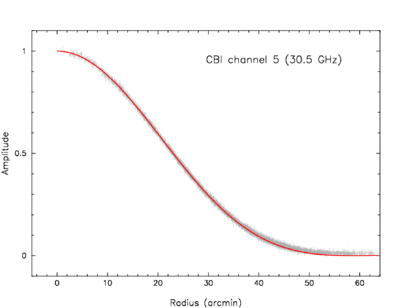
Figure 1.— Radial profile of the CBI primary beam in one of the ten frequency channels; data from all 78 baselines are superimposed. The observations (error bars) were made on 2000 Nov 12; Tau A was observed for about 20 s at each point on a $13\times 13$ grid in azimuth and elevation. The grid points were separated by 7′, so the grid extended to $\pm 42\arcmin$. Measurements within 45′ of the central position were used to fit for the amplitude scale and pointing offset (3 parameters) for each of the 780 datasets (78 baselines $\times$ 10 channels). The red curve shows the adopted profile, which was computed by taking the square of the Fourier transform of the aperture illumination pattern, assumed to be circularly symmetric. Taking the outer radius of the aperture (0.45 m) as $r=1$, the inner part $r<0.172$ is blocked by the secondary and is assumed to have zero illumination. The illumination is tapered from center to edge: we approximate this as a Gaussian $\exp[-(r/r_{0})^{2}]$. The parameter $r_{0}=0.683$ was chosen to give the best fit to all ten channels. It corresponds to an edge taper of $-18.6$ dB and a beam FWHM of $\theta_{\rm FWHM}=45\farcm 2\times(31\,{\rm GHz}/\nu)$. The 13 antennas have very similar beams, but they have relative pointing offsets of 1–2′, up to 5′ in the worst case.

The CBI Cassegrain antennas have a diameter of 0.90 m and a measured primary beam width $\theta_{\rm FWHM}=45\farcm 2\times(31\,{\rm GHz}/\nu)$ at frequency $\nu$, so that $\Delta\ell\approx 300$. The primary beam is quite close to a circular Gaussian, but we have adopted a more accurate model of the radial profile (see Fig. 1) and used this model when making images and estimating the CMB power spectrum.

In observations from a single pointing (as in Paper I and Paper II), the resolution in $\ell$ of the power spectrum is limited to $\sim\Delta\ell$, which is insufficient to resolve the expected structure in the spectrum. To improve the resolution in $\ell$, which is inversely proportional to the angular size of the imaged region, we make mosaiced observations in which we map a larger area of sky using several closely-spaced pointings. This method is in widespread use for making images of extended regions with radio interferometers (e.g., Cornwell, 1988; Sault, Staveley-Smith, & Brouw, 1996). In the observations reported here, we mapped three separate mosaic fields in this way, using 42 pointings for each in a rectangular grid of 7 rows separated by $20\arcmin$ in declination and 6 columns separated by $1\mbox{${}^{\mathrm{m}}$}20\mbox{${}^{\mathrm{s}}$}\approx 20\arcmin$ in right ascension. This allows us to improve the resolution in $\ell$ to $\Delta\ell\approx 100$.

Although the CBI antennas were designed to have low sidelobes and crosstalk (Padin et al., 2000), emission from the ground contaminates the data, especially on short baselines (Padin et al. 2002; Paper I; Paper II). The ground signal is stable on time-scales of many minutes, so if we observe two nearby fields under similar ground conditions, the difference of the visibilities of the two fields is unaffected by the ground. Differencing also eliminates any constant or slowly varying instrumental offsets. We observe a field (the lead field) for about 8 min and then switch to a reference field (trail field), at the same declination but 8 min later in right ascension, for the next 8 min, and form the difference of corresponding $8.4$ s integrations. One such “scan” consists of up to 50 differenced integrations, the exact number depending on how much time is lost to slewing and calibration. The two fields are observed over the same range of azimuth and elevation, so they have nearly identical ground contributions. All the results presented in this paper are derived from the differenced visibilities. The images show the difference of intensity between a region of sky and one 8 min later in right ascension; and the differencing is included in the covariance matrices used for power-spectrum estimation.

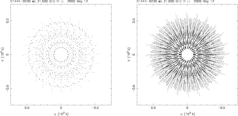
Figure 2.— Typical $(u,v)$ sampling obtained for a single pointing (C1444$-$0230). For this observation only 12 antennas were used. Left: sampling for a single frequency channel. Right: sampling with 10 channels; a separate dot has been used for each channel. The different channels are sensitive to slightly different angular scales.

For each pointing incorporated in the mosaics we obtained approximately 16 such 8 min lead-trail scans, although the exact number varied from one pointing to another. Between scans, we rotated the platform to change its orientation relative to the hour circle, thus improving the sampling of the $(u,v)$ plane. This also reduces the effect of any residual ground contamination: the ground signal does not add coherently when the visibilities from different baselines measuring the same $(u,v)$ point are combined, because the antennas have different far sidelobe responses. An example of the $(u,v)$ plane sampling obtained for a single pointing is shown in Figure 2. No attempt was made to obtain identical sampling for all the pointings.

3. Observations

3.1. Summary of the dataset

In this paper we present observations of three mosaic fields (identified as 02^h, 14^h, and 20^h) separated by about 6^h in right ascension at a declination of about $-3\fdg 5$. The fields were chosen to have IRAS 100 $\mu$m emission less than 1 MJy sr^-1, low synchrotron emission, and no point sources brighter than a few hundred mJy at 1.4 GHz (Condon et al., 1998). Details of the fields observed are given in Table 3. Two of the individual pointings comprising our mosaics have been observed to much greater depth, and our data for these two pointings are a subset of the data analyzed in Paper II.

Data acquisition, calibration, and editing were performed in the manner described in Paper II; we give only a summary here. Observations were made at elevations $>42\arcdeg$, at night, and more than $60\arcdeg$ from the moon. The amplitude scale was based on nightly observations of calibration sources (Jupiter, Saturn, Tau A [3C 144, the Crab Nebula], and Vir A [3C 274]); the primary calibrator was Jupiter, for which we assumed an effective temperature of $152\pm 5$ K at 32 GHz (Mason et al., 1999). We estimate that the overall calibration uncertainty is $5\%$ rms, equivalent to $10\%$ in CMB power. A small fraction of the data were discarded owing to instrumental problems. Most of these problems were detected by real-time monitoring of the receivers; a few hardware problems in the correlators were indicated by unusually high correlation between the real and imaginary parts of the visibility. A few nights were affected by bad weather, and we deleted all data taken at times when atmospheric noise was visible on the short baselines.

As mentioned above, all the data were taken in pairs of 8 min scans on a lead and a trail field, separated by 8 min in RA. The field separation on the sky varied with declination, but for our declinations, $\approx-3\fdg 5$, it was very close to $2\arcdeg$. Individual 8.4 s integrations in the two scans were matched in hour angle and differenced, and unmatched integrations were discarded. We estimated the noise in each scan from the rms of the differenced integrations, and compared it with the expected rms noise level in either the real or imaginary visibility:

$$\sigma={\sqrt{2}k_{\rm B}T_{\rm sys}\over A\eta_{Q}\sqrt{\Delta\nu\tau}},$$ (4)

where $k_{\rm B}$ is Boltzmann’s constant, $T_{\rm sys}$ is the system temperature, $A$ is the effective area of each antenna, $\eta_{Q}$ is the correlator efficiency, $\Delta\nu$ is the channel bandwidth, and $\tau$ is the integration time (Thompson, Moran, & Swenson, 2001). Under good conditions the measured noise, $\sigma\approx 4.7$ Jy s^1/2, is consistent with the estimated system temperature $\approx 30$ K. The rms noise in the differenced data should be $\sqrt{2}\sigma$. When the rms exceeded 2.6 times the expected rms, we discarded the entire scan-pair. This eliminated almost all of the data affected by the atmosphere. A final visibility estimate for each channel of each baseline in each orientation of the antenna platform was computed by a weighted average of the individual scan visibilities, and the uncertainty in this estimate was computed from the scan rms’s, taking into account a bias introduced by the fact that the scan rms’s are themselves estimated from the data (see Paper II).

The final edited and calibrated dataset is summarized in Table 3, which reports the total integration time (averaged over baselines) on each of the lead and trail fields comprising the mosaics. Owing to the vagaries of the weather and the telescope, some fields were observed to greater depths than others, and a few were missed altogether; this is reflected in the variation of sensitivity across each mosaic (see § 3.3).

3.2. Foreground Point Sources

In the 26–36 GHz band, the dominant confusing foreground is the emission from discrete radio galaxies and quasars, which we refer to as “point sources” (they are virtually unresolved by the CBI). The contribution of point sources to the visibilities must be removed in order to obtain a reliable estimate of the CMB power spectrum. A random distribution of point sources has a power spectrum $C_{\ell}={\rm constant}$, while for the CMB $C_{\ell}$ decreases rapidly with increasing $\ell$, so discrete sources dominate at high $\ell$.

To remove most of the point-source contamination in our data, we measured the flux densities of a large number of known point sources in the mosaic fields using a new dual-beam 31 GHz HEMT receiver with a beamwidth of $81\arcsec$ on the 40-meter telescope at the Owens Valley Radio Observatory (OVRO). The observations followed standard methods (see, e.g., Myers, Readhead, & Lawrence 1993); details will be presented elsewhere (B. S. Mason et al., in preparation). A total of 2225 sources brighter than 6 mJy at 1.4 GHz in the NRAO VLA 1.4 GHz Sky Survey (NVSS; Condon et al. 1998) were observed, as described in Paper II. For each source detected above a $4\sigma$ threshold, the expected visibility (assuming a point source at the NVSS position with the OVRO flux density attenuated by the CBI primary beam) was subtracted from the CBI visibility data. The survey is 90% complete for $S_{31\,\rm GHz}>16$ mJy and 99% complete for $S_{31\,\rm GHz}>21$ mJy. A total of 70 sources were subtracted from the 02^h data, 63 from the 14^h data, and 68 from the 20^h data. To estimate the response in each CBI frequency channel, we used the two-point spectral index $\alpha$ (1.4–31 GHz) for steep-spectrum sources ($\alpha<-0.5$ where $S_{\nu}\propto\nu^{\alpha}$) and an average spectral index $\alpha=-0.23$ for the remainder, which may be variable; but as we are only extrapolating $\pm 16\%$ in frequency the results are not very sensitive to the choice of $\alpha$.

By making images before and after source subtraction (see § 3.3) we have verified that the CBI and OVRO measurements are consistent. The resulting images are dominated by the CMB. However, source subtraction is not sufficient for accurate power-spectrum estimation, because there may be small residuals and there will also be unmeasured sources that have not been accounted for. When estimating the CMB power spectrum, we have adopted a more powerful method than source subtraction: we have projected out the known point sources (following Halverson et al. 2002) (see § 4.2). Although we subtracted the sources measured at OVRO, we also projected them out, so errors in the OVRO flux-density measurements should not affect the power spectrum estimates.

3.3. Images

The quantity of primary cosmological interest, the power spectrum, is best estimated directly from the visibility data, as discussed in § 4 below. However, we can also make images of the CMB (convolved with the instrumental point-spread function) by Fourier-transforming the visibilities. The images provide a good check for the presence of non-gaussian features in the CMB or instrumental errors in the data, such as calibration errors (which would show up as residuals after point-source subtraction).

We have used standard aperture-synthesis techniques (Taylor, Carilli, & Perley, 1999) to make images from each pointing. The images are formed from linear combinations of the measured visibilities and we have not done any deconvolution or “cleaning.” The “dirty” image $I_{D}$ is the Fourier transform of the sampled visibilities,

$$I_{D}(\mbox{\boldmath{$x$}})={\sum_{k}w_{k}\left\{V_{k}^{R}\cos[2\pi\mbox{\boldmath{$u$}}_{k}\cdot\mbox{\boldmath{$x$}}]-V_{k}^{I}\sin[2\pi\mbox{\boldmath{$u$}}_{k}\cdot\mbox{\boldmath{$x$}}]\right\}\over\sum_{k}w_{k}},$$ (5)

and is the convolution of $A(\mbox{\boldmath{$x$}})I(\mbox{\boldmath{$x$}})$ (the primary beam response times the sky brightness) with the point-spread function or dirty beam $B_{D}(\mbox{\boldmath{$x$}})$:

$$B_{D}(\mbox{\boldmath{$x$}})={\sum_{k}w_{k}\cos[2\pi\mbox{\boldmath{$u$}}_{k}\cdot\mbox{\boldmath{$x$}}]\over\sum_{k}w_{k}}.$$ (6)

In practice, we resample the visibilities on a grid and use an FFT to compute the image and beam using standard software (Shepherd, 1997). The sky coordinates $x$ are the Fourier conjugates to the baseline components $u$ and correspond to direction cosines relative to the pointing center. The weights $w_{k}$ are usually chosen to be the statistical weights (“natural weighting”), $w_{k}=1/\sigma_{k}^{2}$ where $\sigma_{k}$ is the standard deviation of the real or imaginary part of the complex visibility, estimated as described above. With this weighting, the variance of the dirty image is

$$s^{2}=\langle{[I_{D}(\mbox{\boldmath{$x$}})-\langle{I_{D}(\mbox{\boldmath{$x$}})}\rangle]^{2}}\rangle={1\over\sum_{k}\sigma_{k}^{-2}}.$$ (7)

A “linear” mosaic image $I_{M}(\mbox{\boldmath{$x$}})$ is formed from several pointings by shifting each dirty image to a common phase center, correcting it for its primary beam, and making a weighted sum at each pixel:

$$I_{M}(\mbox{\boldmath{$x$}})={\sum_{p}W_{p}(\mbox{\boldmath{$x$}}){I_{D,p}(\mbox{\boldmath{$x$}})/A_{p}(\mbox{\boldmath{$x$}})}\over\sum_{p}W_{p}(\mbox{\boldmath{$x$}})}.$$ (8)

The weighted mean gives a maximum-likelihood estimate if the weights are equal to the inverse variances of the corrected images, i.e., $W_{p}(\mbox{\boldmath{$x$}})=A_{p}^{2}(\mbox{\boldmath{$x$}})/s^{2}_{p}$, where $s^{2}_{p}$ is the variance of the dirty image made from the $p$th pointing. Thus

$$I_{M}(\mbox{\boldmath{$x$}})={\sum_{p}A_{p}(\mbox{\boldmath{$x$}})I_{D,p}(\mbox{\boldmath{$x$}})/s_{p}^{2}\over\sum_{p}A_{p}^{2}(\mbox{\boldmath{$x$}})/s_{p}^{2}},$$ (9)

and the variance in the mosaic image is

$$\sigma_{M}^{2}(\mbox{\boldmath{$x$}})={1\over\sum_{p}A_{p}^{2}(\mbox{\boldmath{$x$}})/s_{p}^{2}}$$ (10)

(Cornwell, 1988; Sault, Staveley-Smith, & Brouw, 1996). The variance varies across the image, and it is necessary to truncate the image where the variance becomes excessive. We have used the model for the primary beam described in the caption to Figure 1, set to zero for radii $>90\arcmin$. In making the mosaic images, and in the power spectrum analysis described below, we have made the approximation that the sky is flat over the $\sim 3\arcdeg$ image, which is equivalent to an error of $<5\arcdeg$ of phase on the longest baselines.

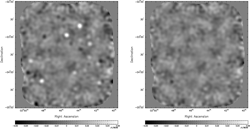
Figure 3.— Images of the 02^h mosaic. Left: raw data; right: after subtraction of sources measured at OVRO. The images show the difference of the emission in the lead and trail fields. The coordinates are J2000. The right ascension scale applies to the lead field; add 8^m to obtain the right ascension of objects in the trail field. The same gray-scale range has been used for both images, and it does not show the full brightness range of the discrete sources. Light (positive) spots are discrete sources in the lead field, while dark (negative) spots are discrete sources in the trail field. The brightest source in this image has a flux density of about 67 mJy at 31 GHz. These images were made from the entire dataset using natural weighting, and they have been corrected for the primary beam response as described in § 3.3. They have a resolution (FWHM) of $5\farcm 2$–$5\farcm 5$ (the resolution varies slightly across the image, depending on the $(u,v)$ coverage obtained for each pointing).

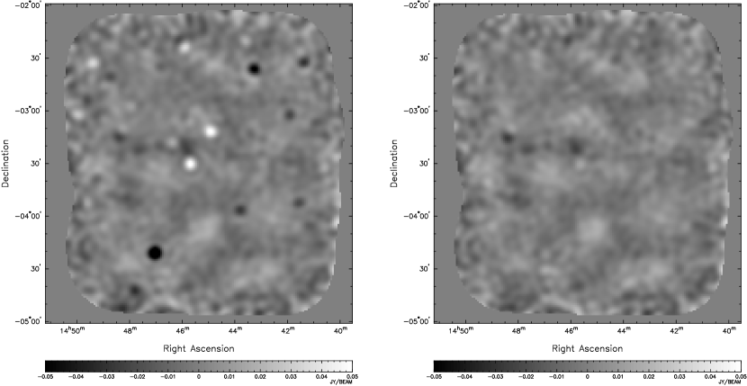
Figure 4.— Images of the 14^h mosaic. Left: raw data; right: after subtraction of sources measured at OVRO. For details, see caption to Fig. 3.

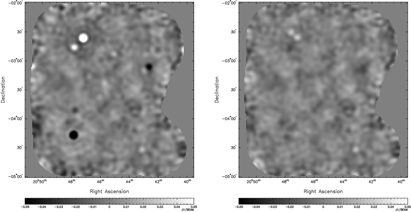
Figure 5.— Image of the 20^h mosaic. Left: raw data; right: after subtraction of sources measured at OVRO. For details, see caption to Fig. 3.

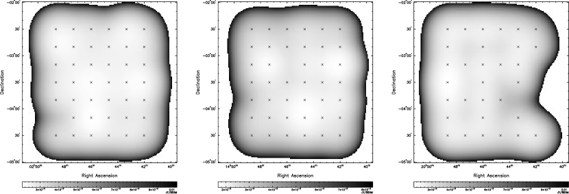
Figure 6.— The variation of rms noise level $\sigma_{M}$ across each mosaic image (see equation 10). The pointing centers are marked with $\times$. The outer parts of the images, where the noise level exceeds a specified threshold, have been blanked. In the 02^h and 20^h mosaics, the minimum noise level is 2.0 mJy/beam and the blanking threshold is 10 mJy/beam. The corresponding numbers are 1.7 and 8.3 mJy/beam for the 14^h mosaic. The sky areas covered within these thresholds are 7.45 (02^h), 7.13 (14^h), and 7.20 (20^h) deg² in each of lead and trail.

Figures 3–9 show mosaic images made from the CBI data. We can make a variety of different images by selecting different subsets of the data and adjusting the weights $w_{k}$.

Figures 3, 4, and 5 show mosaic images made from the entire dataset using natural weighting, and similar images made from the visibility data after subtraction of the point sources measured at OVRO. Figure 6 shows the variation of noise level across these images, and indicates the pointing centers. The effectiveness of the OVRO source subtraction can be seen by comparison of the “before” and “after” images. Most of the sources have been removed successfully, although there are of course residuals owing to measurement errors or source variability, and a few sources can be seen that were not detected at OVRO (these sources were projected out in the power spectrum analysis).

To investigate the sources further, we have made higher-resolution images (not shown) using only baselines longer than 250$\lambda$, and searched for peaks exceeding $5\sigma_{M}$ in images of signal-to-noise ratio. All these peaks are coincident within $2\arcmin$ with sources that have $S_{1.4\,\rm GHz}>3.4$ mJy in the NVSS catalog. Of the 42 sources detected, 37 are identified with NVSS sources with $S_{1.4\,\rm GHz}>6$ mJy which were detected at OVRO. The remaining five objects are associated with NVSS sources that were not detected at OVRO; one of them, with $S_{1.4\,\rm GHz}<6$ mJy, was not observed at OVRO. As we reported in Paper II, we find that the number $N$ of sources greater than flux density $S$ at 31 GHz is

$$N(S)\approx 2.8\pm 0.7\,{\rm deg}^{-2}\left(S\over 10\,{\rm mJy}\right)^{-1.0}$$ (11)

for $5<S<50$ mJy. We use this result in § 4.2 to estimate the contribution to our power spectra of sources below $S_{1.4\,\rm GHz}>3.4$ mJy (stronger sources are treated individually).

Figures 9, 9, and 9 show lower-resolution images made by reducing the weight of long baselines with a Gaussian taper; this suppresses the high-frequency noise and emphasizes the CMB emission. These figures include images made from the upper and lower halves of the CBI frequency band. There is good visual correspondence between the two halves of the band; but note that the spatial-frequency sampling is not the same in the two halves, so a quantitative comparison is difficult. The visual agreement is echoed in the good agreement between the power spectra obtained from the two halves of the band (see § 4.3.4). These low-resolution images are dominated by sky signal rather than noise. Note, however, that the images are differences of two sky patches, and they are also missing the lowest spatial frequencies, so a comparison with images obtained with another instrument may be difficult. By inspection of signal-to-noise ratio images (computed using Eqs. 9 and 10) made from subsets of the data, we have found that signals corresponding to $\ell\lesssim 1000$ are detected with high significance ($\gtrsim 3\sigma$), and there are some significant detections of individual features at higher $\ell$. The detected features range in angular size from $\sim 6\arcmin$ to $\sim 15\arcmin$, corresponding to mass scales at the surface of last scattering of $\sim 5\times 10^{14}$ to $8\times 10^{15}\,M_{\sun}$, so these features are likely to be the seeds that would evolve into clusters of galaxies by the present epoch.

4. Power Spectrum

4.1. Algorithm

Our algorithm for the estimation of power spectra from mosaic visibility data is described in Paper IV. We model the power spectrum as flat in each of a set of $N_{B}$ contiguous bands, i.e.,

$${\cal C}_{\ell}\equiv\ell(\ell+1)C_{\ell}/2\pi=q_{B},\quad\ell_{B-1}<\ell<\ell_{B}$$ (12)

(with $\ell_{0}=0$), and take the band-powers $q_{B}$ ($B=1,\ldots,N_{B}$) as a set of unknown parameters to be determined by maximizing the likelihood (the probability of obtaining the measured visibilities, if the model were correct, for given values of the parameters). If the signal and noise obey Gaussian statistics, which we assume, the likelihood is given by the multivariate Gaussian distribution for complex variates,

$${\cal L}(q_{B})={1\over\pi^{n}\det\mbox{{$\bf C$}}}\exp\left(-\mbox{\boldmath{$V$}}^{\dagger}\mbox{{$\bf C$}}^{-1}\mbox{\boldmath{$V$}}\right),$$ (13)

where $V$ is a column vector containing the complex visibility measurements, $\mbox{{$\bf C$}}=\langle\mbox{\boldmath{$V$}}\mbox{\boldmath{$V$}}^{\dagger}\rangle$ (a function of the parameters $q_{B}$) is the covariance matrix of the visibilities, and ^† denotes the Hermitian conjugate. (Although eq. [13] is expressed in terms of complex visibilities, it is easier in practice to treat the real and imaginary parts of the visibilities as a double-length real vector).

The correlation matrix $\bf C$ can be written as

$$\bf C = \mbox{{$\bf C$}}^{\rm N}+\sum_{B}q_{B}\mbox{{$\bf C$}}_{B}^{\rm S}+q_{\rm res}\mbox{{$\bf C$}}^{\rm res}$$ (14)

$$+q_{\rm OVRO}\mbox{{$\bf C$}}^{\rm OVRO}+q_{\rm NVSS}\mbox{{$\bf C$}}^{\rm NVSS},$$

where $\mbox{{$\bf C$}}^{\rm N}$ is the noise correlation matrix, estimated from the data as described above, $\mbox{{$\bf C$}}_{B}^{\rm S}$ is the CMB signal correlation matrix for band $B$ (independent of $q_{B}$), $\mbox{{$\bf C$}}^{\rm OVRO}$ and $\mbox{{$\bf C$}}^{\rm NVSS}$ are constraint matrices (Bond, Jaffe, & Knox, 1998) representing the effects of foreground point sources of known position, and $\mbox{{$\bf C$}}^{\rm res}$ represents a residual contribution from faint sources of unknown position. We discuss the source terms further in § 4.2. The factors $q_{\rm res}$, $q_{\rm OVRO}$, and $q_{\rm NVSS}$ could in principle be regarded as free parameters to be determined by maximum likelihood, but in practice they are not well determined by the data and we instead hold them fixed at a priori values.

In a typical mosaic observation, the number of distinct visibility measurements is very large ($\sim 200\,000$ complex visibilities for a mosaic of 42 pointings with 10 frequency channels, 78 baselines, and several parallactic angles), which makes the covariance matrices (eq. [14]) impractically large. However, neighboring points in the $(u,v)$ plane are highly correlated and need not be treated completely independently. To reduce the size of the matrices, we interpolate the measured visibility set $V$ onto a smaller number of grid points in the $(u,v)$ plane (so that the quantities that enter the likelihood calculation are linear combinations of the measured visibilities), and make the corresponding transformation of the covariance matrix. By this means we reduce the dimension of the (real) matrices to $\lesssim 5000$. We ran tests with different grid spacings, using both real data and simulated data, to verify that using a finer grid would not significantly change the results (see Paper IV). We find the maximum likelihood solution by the quadratic relaxation technique of Bond, Jaffe, & Knox (1998), which yields estimates of the band powers $q_{B}$, with their covariances given by the inverse of the Fisher information matrix

$$F_{BB^{\prime}}=\left\langle{\partial^{2}\ln{\cal L}\over\partial q_{B}\partial q_{B^{\prime}}}\right\rangle={1\over 2}{\rm Tr}\left(\mbox{{$\bf C$}}^{-1}\mbox{{$\bf C$}}_{B}^{\rm S}\mbox{{$\bf C$}}^{-1}\mbox{{$\bf C$}}_{B^{\prime}}^{\rm S}\right).$$ (15)

We also calculate the band-power window functions and the equivalent band-powers of the noise, known point sources, and residual point sources by the methods described in Paper IV. The band-power window function $W^{B}(\ell)$ (Knox, 1999) allows the expected band-power for a given model power spectrum to be estimated as a weighted mean:

$$\langle q_{B}\rangle=\sum_{\ell}{\cal C}_{\ell}{W^{B}(\ell)\over\ell}.$$ (16)

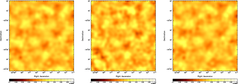
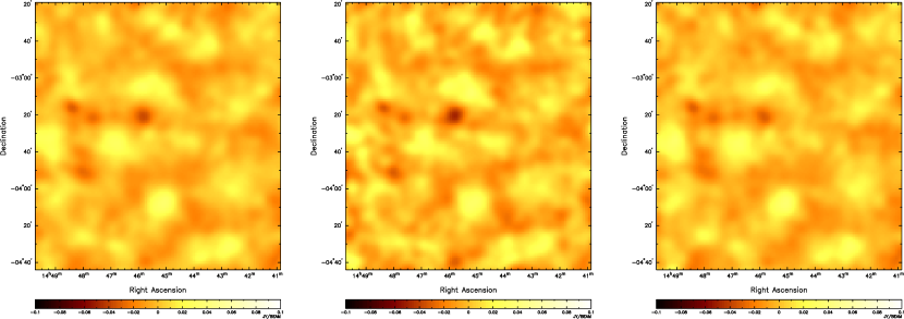
Figure 7.— Central part of the 02^h mosaic, imaged with lower resolution, after subtraction of sources measured at OVRO. A Gaussian taper has been applied to the visibilities, falling to 0.1 at a baseline length of 500 wavelengths. Left: all frequency channels (26–36 GHz); beam FWHM $\approx 6.9\arcmin$. Center: high-frequency channels (31–36 GHz); beam FWHM $\approx 6.6\arcmin$. Right: low-frequency channels (26–31 GHz); beam FWHM $\approx 7.1\arcmin$.

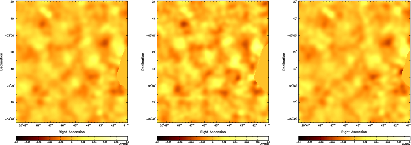
Figure 8.— Central part of the 14^h mosaic, imaged with lower resolution, after subtraction of sources measured at OVRO. A Gaussian taper has been applied to the visibilities, falling to 0.1 at a baseline length of 500 wavelengths. Left: all frequency channels (26–36 GHz); beam FWHM $\approx 6.9\arcmin$. Center: high-frequency channels (31–36 GHz); beam FWHM $\approx 6.6\arcmin$. Right: low-frequency channels (26–31 GHz); beam FWHM $\approx 7.1\arcmin$.

Figure 9.— Central part of the 20^h mosaic, imaged with lower resolution, after subtraction of sources measured at OVRO. A Gaussian taper has been applied to the visibilities, falling to 0.1 at a baseline length of 500 wavelengths. Left: all frequency channels (26–36 GHz); beam FWHM $\approx 6.9\arcmin$. Center: high-frequency channels (31–36 GHz); beam FWHM $\approx 6.6\arcmin$. Right: low-frequency channels (26–31 GHz); beam FWHM $\approx 7.1\arcmin$.

4.2. Correction for Foreground Point Sources

If we had accurate measurements of all the point sources in our frequency band, we could subtract their contributions directly from the visibilities, but as we do not we must adopt a statistical approach. A detailed description of our method of dealing with point sources is presented in Paper II, and here we give only a summary.

The strongest sources (“OVRO” sources) were measured at OVRO and subtracted from the visibility data as described above. The subtraction was necessarily imperfect, however, and the residuals of the subtracted sources make a contribution to the power spectrum that must be removed. We created a second list of “NVSS” sources within about $60\arcmin$ of any of the mosaic pointing centers that were not detected at OVRO but had $S_{1.4\,\rm GHz}>3.4$ mJy, which corresponds to $S_{31\,\rm GHz}>0.25$ mJy for a typical spectral index of $-0.84$. This list contained 960, 918, and 974 sources in the 02^h, 14^h, and 20^h mosaic fields. Crude estimates of the flux densities for these sources were subtracted from the visibilities as part of the power-spectrum estimation. For each mosaic, we constructed two constraint matrices, $\mbox{{$\bf C$}}^{\rm OVRO}$ and $\mbox{{$\bf C$}}^{\rm NVSS}$, using the positions and estimated residual flux-density uncertainties of the sources in the two lists. In principle, if our error estimates were correct, the constraint matrices would fully account for the source contributions and should be included in the maximum likelihood analysis with prefactors $q_{\rm OVRO}=q_{\rm NVSS}=1$. However, after some experimentation, we decided to err on the side of caution and use large prefactors, $q_{\rm OVRO}=q_{\rm NVSS}=10^{5}$, to give very low weight to modes that are affected by these known sources (much larger factors cause the covariance matrix to be ill-conditioned). This is equivalent to marginalizing over the unknown flux densities, or “projecting out” the sources (Halverson et al., 2002; Bond, Jaffe, & Knox, 1998). Our analysis is thus insensitive to errors in the assumed flux densities of the sources, but at the cost of some loss in sensitivity (see Paper IV).

Sources that are not included in the known-source lists also contribute power. We estimate the visibility covariance arising from such sources and include it as the residual source term $\mbox{{$\bf C$}}^{\rm res}$. The radio source counts and spectra used to compute this term are described in Paper II. As in that paper, we estimate that, for an NVSS flux-density cutoff at $S_{1.4\,\rm GHz}>3.4$ mJy, the amplitude of the residual correction is $C_{\nu}^{\rm res}=0.08\pm 0.04$ Jy² sr^-1 (see Paper IV). The dividing line between known sources and sources included in the residual term is somewhat arbitrary, so long as the residual term is computed correctly for the chosen flux-density cutoff. We have conducted tests to verify that our results are insensitive to the precise choice of cutoff. For a full discussion of the source projection and the residual correction, see Paper II.

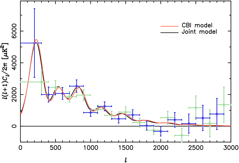
Figure 10.— Joint power spectrum estimates for the three CBI mosaics. Band-power estimates have been made for two alternate divisions of the $\ell$ range into bins: “even” binning (green squares) and “odd” binning (blue circles). The error-bars show $\pm 1\sigma$ uncertainties from the inverse Fisher matrix. Two minimal inflation-based models are shown. Red: fit to CBI plus COBE DMR; $\Omega_{\rm tot}=1.0$, $\Omega_{b}h^{2}=0.0225$, $\Omega_{\rm cdm}h^{2}=0.12$, $\Omega_{\Lambda}=0.6$, $n_{s}=0.95$, $\tau_{c}=0.025$, ${\cal C}_{10}=786$ $\mu$K². Black: joint fit to CBI, DMR, DASI, BOOMERANG-98, VSA and earlier data; $\Omega_{\rm tot}=1.0$, $\Omega_{b}h^{2}=0.02$, $\Omega_{\rm cdm}h^{2}=0.14$, $\Omega_{\Lambda}=0.5$, $n_{s}=0.925$, $\tau_{c}=0$, ${\cal C}_{10}=887$ $\mu$K². For details, see Paper V.

Table 1Band-Powers and Uncertainties

$\ell$ range	$\ell_{\rm eff}$	Band-Power $l(l+1)C_{l}/(2\pi)$ ($\mu$K2)
0–400	304	2790 $\pm$ 771
400–600	496	2437 $\pm$ 449
600–800	696	1857 $\pm$ 336
800–1000	896	1965 $\pm$ 348
1000–1200	1100	1056 $\pm$ 266
1200–1400	1300	685 $\pm$ 259
1400–1600	1502	893 $\pm$ 330
1600–1800	1702	231 $\pm$ 288
1800–2000	1899	$-$250$\pm$ 270
2000–2200	2099	538 $\pm$ 406
2200–2400	2296	$-$578$\pm$ 463
2400–2600	2497	1168 $\pm$ 747
2600–2800	2697	178 $\pm$ 860
2800–3000	2899	1357 $\pm$ 1113
0–300	200	5243 $\pm$ 2171
300–500	407	1998 $\pm$ 475
500–700	605	2067 $\pm$ 375
700–900	801	2528 $\pm$ 396
900–1100	1002	861 $\pm$ 242
1100–1300	1197	1256 $\pm$ 284
1300–1500	1395	467 $\pm$ 265
1500–1700	1597	714 $\pm$ 324
1700–1900	1797	40 $\pm$ 278
1900–2100	1997	$-$319$\pm$ 298
2100–2300	2201	402 $\pm$ 462
2300–2500	2401	163 $\pm$ 606
2500–2700	2600	520 $\pm$ 794
2700–2900	2800	770 $\pm$ 980

4.3. Results

4.3.1 Joint Mosaic Power Spectrum

The primary result of this paper is the power spectrum of the CMB in the three mosaics treated jointly. For this analysis we have estimated the power spectrum in bins of width $\Delta\ell=200$, with two alternate locations of the bins. The “even” binning has $\ell_{B}=200+200B$ ($1\leq B\leq 16$), while the “odd” binning has $\ell_{B}=100+200B$ ($1\leq B\leq 16$); here $\ell_{B}$ is the upper limit of the bin, as in equation (12). In both cases the first bin is wider and starts at $\ell=0$. While we included bins at higher $\ell$, we report the results only for $\ell<3000$: at higher $\ell$, the mosaic data have very little sensitivity. The two sets of bins are of course not independent. The results are given in Table 1, which gives for each bin the band-power $q_{B}$, the rms uncertainty in $q_{B}$ from the Fisher matrix, and the centroid of the window function $\ell_{\rm eff}$. The results are also displayed in Figure 10, and the window functions are shown in Figure 11. With $\Delta\ell=200$, the adjacent bins are anticorrelated by about $16\%$. We have also computed power-spectrum estimates using narrower bins with $\Delta\ell=140$, for which the anticorrelation of adjacent bins is about $24\%$, again using overlapping “odd” and “even” bins. We have used all four binnings ($\Delta\ell=140$ odd and even, and $\Delta\ell=200$ odd and even) for cosmological-parameter estimation (see Paper V), and all four give consistent results. The component band-powers (defined in Paper IV) for instrumental thermal noise ($\mbox{{$\bf C$}}^{\rm N}$) and the residual source correction ($\mbox{{$\bf C$}}^{\rm res}$) are shown in Figure 12. This figure shows that the residual source correction is negligible at $\ell\lesssim 2000$; the thermal noise, however, exceeds the signal for $\ell>1300$ and is the dominant effect at high $\ell$. Both these corrections increase approximately, but not exactly, as $\ell^{2}$. The thermal noise depends on the sampling in the $(u,v)$ plane and better-sampled $\ell$ bins have lower noise; while the residual source correction has a non-thermal spectrum and the magnitude of its contribution in any bin depends on the spectral sensitivity in that bin—this varies from bin to bin as the CBI frequency channels do not have the same $(u,v)$ sampling.

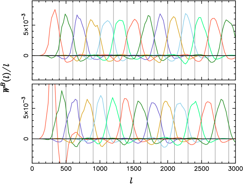
Figure 11.— Window functions for the joint power spectrum estimates for the three CBI mosaics. Top: “even” binning. Bottom: “odd” binning. The vertical grey lines show the bin boundaries. Each function is normalized: $\sum_{\ell}W^{B}(\ell)/\ell=1$.

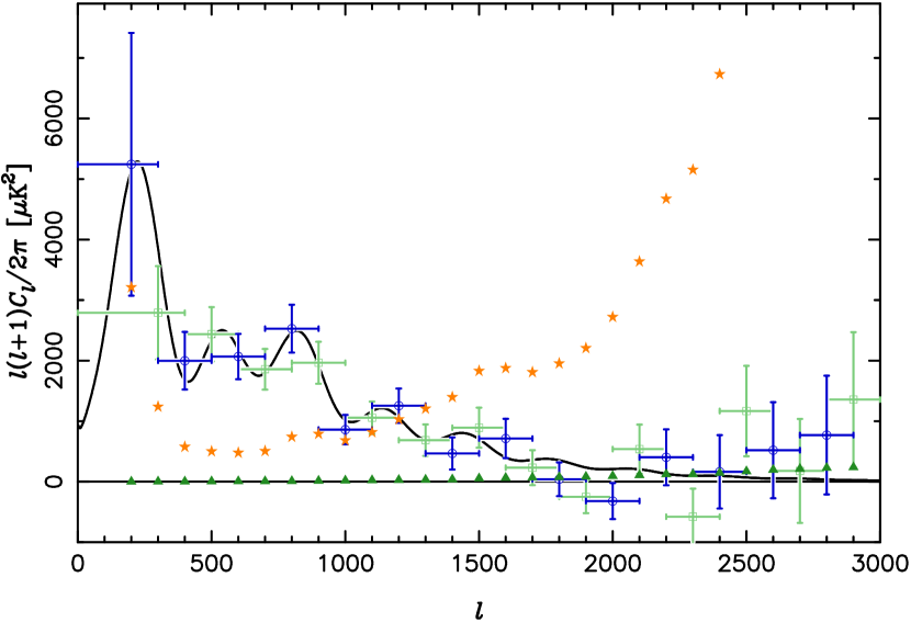
Figure 12.— Joint power spectrum estimates for the three CBI mosaics (the same as Fig. 10). The stars represent the power spectrum of the instrumental noise correction, and the triangles represent the power spectrum of the residual source correction. The black curve is the joint model from Figure 10.

Figure 10 shows two theoretical spectra for minimal inflation-based models with different parameters. As we discuss in Paper V, we have evaluated the posterior probabilities of the CBI and other datasets over a grid of models in a 7-dimensional parameter space, using a variety of prior probabilities based on Hubble constant, large-scale-structure, and supernova-Ia observations. The first model displayed in Figure 10 is the model that maximizes the posterior probability of the CBI mosaic (using the “odd” $\Delta\ell=140$ binning) and COBE-DMR results, with the weak-$h$ prior on the Hubble constant; within the grid of models, this is also the best fit if we restrict the search to flat models. The second model is intended to represent a current “concordance” model: it is the best fit of the CBI, DMR, DASI, and BOOMERANG-98 data with flat and weak-$h$ priors. We find the same model if we also include LSS, SN, or HST-$h$ priors. The parameters for the two models are given in the figure caption. It is remarkable that the two spectra are so similar. The CBI data together with DMR place strong constraints on the allowed region of parameter space. These constraints are consistent with those obtained from earlier CMB observations, even though the CBI is sampling an $\ell$ range a factor of two larger than that spanned by the earlier experiments. For a full discussion of parameter estimation from the CBI results, see Paper V.

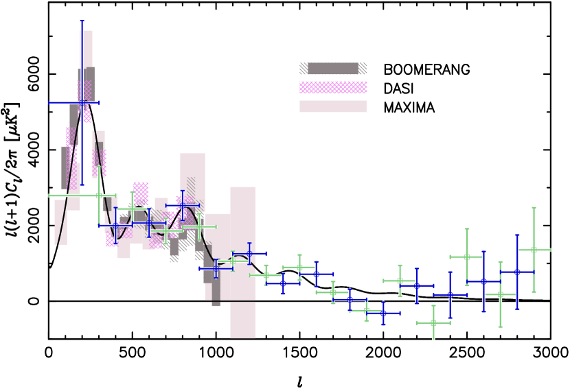
Figure 13.— Comparison of the joint power spectrum estimates from the three CBI mosaics (Fig. 10) with the measurements from BOOMERANG (Netterfield et al., 2002), DASI (Halverson et al., 2002), and MAXIMA (Lee et al., 2001). The rectangles indicate the 68% confidence intervals on band-power; for BOOMERANG, the solid rectangles indicate the 68% confidence interval for the statistical and sample variance errors, while the hatched rectangles shows the amount by which a $\pm 1\sigma$ error in the beamwidth ($12\farcm 9\pm 1\farcm 4$) would shift the estimates (all up or all down together). The black curve is the joint model from Figure 10.

We compare our results with the earlier results from the BOOMERANG, DASI, and MAXIMA experiments in Figure 13. In the region of overlap ($300\lesssim\ell\lesssim 1000$) the agreement is very good. A detailed comparison will be made in Paper V.

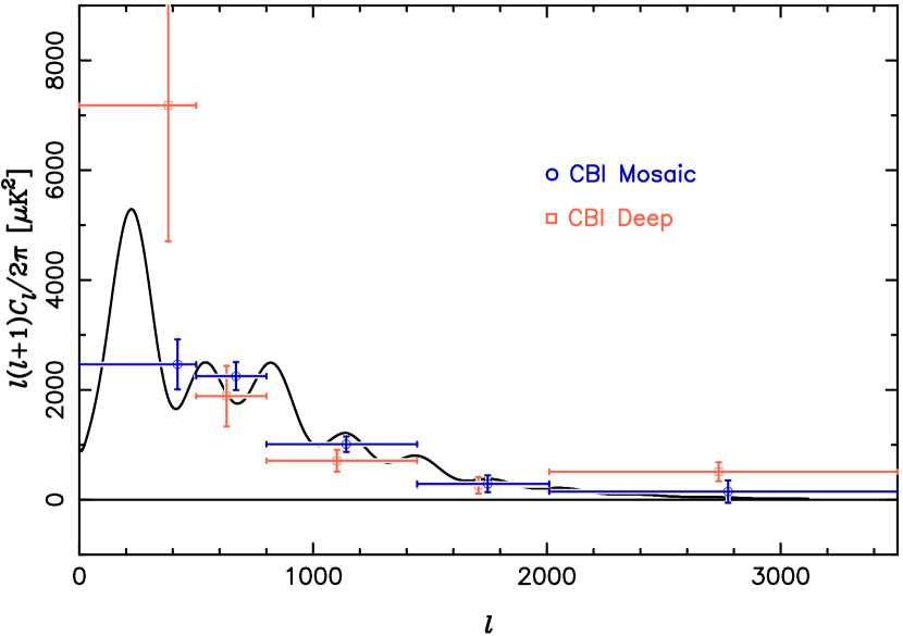
Figure 14.— Comparison of the joint power spectrum estimates from the three CBI mosaics (blue circles) with those from the three deep fields of Paper II (red squares); both have been computed for the $\ell$ bins used in Paper II. The black curve is the joint model from Figure 10.

We have also computed the power spectrum of the three mosaics using the wider bins chosen for analyzing the CBI deep field data (Paper II). The deep and mosaic results are compared in Figure 14. We have used six bins: $\ell=0$–500, 500–800, 880–1445, 1445–2010, 2010–3500, and $\ell>3500$. The last bin contains virtually no data for the mosaics, and we have omitted it from the figure. The first bin ($\ell<500)$) is poorly constrained by the data and has a large uncertainty owing to sample variance. Two of the three deep fields lie within the area covered by the mosaics, so the results are not entirely independent. But if we ignore this complication, we can compare the two sets of band-powers by a chi-squared test, using the band-power covariance matrices. For this test, we assume that the likelihood function is approximately Gaussian and compute

$$\chi^{2}=\sum_{B}\sum_{B^{\prime}}\left(q_{B}^{(1)}-q_{B}^{(2)}\right)\left(M_{BB^{\prime}}^{(1)}+M_{BB^{\prime}}^{(2)}\right)^{-1}\left(q_{B^{\prime}}^{(1)}-q_{B^{\prime}}^{(2)}\right),$$ (17)

where $q_{B}^{(1)},q_{B}^{(2)}$ are the band-power estimates and $M_{BB^{\prime}}^{(1)},M_{BB^{\prime}}^{(2)}$ are the inverse Fisher matrices for the two datasets. Omitting the first and last bins, we find $\chi^{2}=5.57$, with 5 degrees of freedom. If the two data sets were drawn from the same population, a larger value would be obtained in 35% of trials, so we conclude that the two data sets are consistent. At $\ell>2000$, where the deep observations show a significant signal, the mosaic observations are less sensitive than the deep and are consistent both with the deep result and with no signal. In the bin $2010<\ell<3500$, we find $q_{B}=148\pm 203$ $\mu$K² in the mosaics and $q_{B}=510\pm 171$ $\mu$K² in the deep fields. The thermal noise band-power in this bin is much larger for the mosaic data set than for the deep data set, so the deep results are less sensitive to systematic errors in the noise estimation and are thus more reliable than the mosaic results.

4.3.2 Peaks and Dips in the Power Spectrum

The power spectra with bin size $\Delta\ell=200$ (Fig. 10) suggest the presence of peaks and dips, but, owing to the anticorrelations between adjacent bins, their reality is difficult to assess in this presentation, or in similar plots of the $\Delta\ell=140$ bins. To assess their significance, we have searched for extrema in the power spectrum following techniques applied to the BOOMERANG data by de Bernardis et al. (2002). For each triplet of adjacent bins $[i-1,i,i+1]$ we model the local band-power profile as a three-parameter quadratic form

$$q_{B}=a{\ell}^{2}_{B}-2b{\ell}_{B}+c,\quad\quad B=i-1,i,i+1,$$ (18)

where ${\ell}^{2}_{B}$, ${\ell}_{B}$ are band-average values of $\ell^{2}$ and $\ell$. In terms of the fitted parameters $a,b,c$, the peak location is $\ell_{\rm pk}=b/a$, its amplitude is ${\cal C}_{\rm pk}=c-b^{2}/a$, and its curvature $\kappa_{\rm pk}=a$. We have assumed that the measured $q_{B}$’s are Gaussian-distributed with a covariance $F_{BB^{\prime}}^{-1}$. In this Gaussian approximation for the likelihood ${\cal L}(q_{B}$), the likelihood ${\cal L}(a,b,c)$ of the quadratic parameters is also a Gaussian: the maximum values $a_{m},b_{m},c_{m}$ are a direct transform of the data band-power averages in the three bins, and the curvature at the maximum, which describes the uncertainty in these parameter estimates, is simply related to $F_{BB^{\prime}}$. The maximum-likelihood values of $\ell_{\rm pk}$, ${\cal C}_{\rm pk}$ and $\kappa_{\rm pk}$ are determined by $a_{m},b_{m},c_{m}$, but the errors in these transformed variables are non-Gaussian. We estimate the errors by computing the local curvature of the likelihood near maximum, by a Jacobian transformation. We consider a peak or a dip in the spectrum to be detected if two conditions are met: (1) the position $\ell_{\rm pk}$ is within the range of multipoles covered by the band triplet; (2) the best fit quadratic has a curvature $a_{m}$ which differs from zero by at least $1\sigma$.

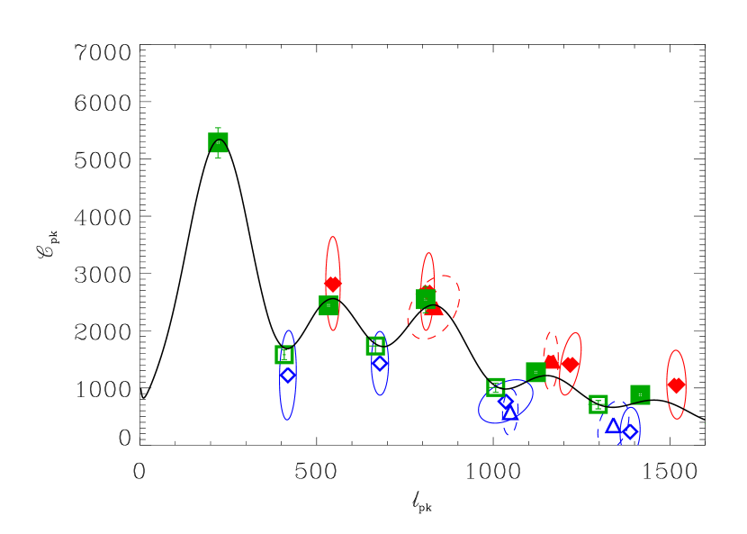
Figure 15.— Results for the peak and dip detection algorithm applied to the $\Delta\ell=140$ data. Peaks (red) and dips (blue) found in the odd binning are indicated by diamonds with ellipses showing the $1\sigma$ confidence contours; those found in the even binning are shown by triangles with dashed confidence contours. Only detections with curvature above $1\sigma$ are shown. For comparison, the filled and open green squares show the peak and dip positions and amplitudes predicted from earlier CMB observations in the context of inflation-motivated models: they are from ensemble averages over the ${\cal C}_{\ell}$-database we use for parameter estimation in Paper V (for the weak-$h$ prior). In this figure the black curve is the CBI+DMR model from Figure 10.

The results of applying this algorithm to the $\Delta\ell=140$ odd and even binned data for $\ell<2000$ are shown in Figure 15. There are more detections in the odd binning than in the even binning, which is an indication that even the $\Delta\ell=140$ bin size is larger than we would like for effective peak/bin detection. In the odd binning, we detect four peaks, at $\ell\sim 550,800,1150,1500$, and four dips, at $\ell\sim 400,700,1050,1400$. The significance levels of the peaks, expressed as $|a_{m}|/\sigma$, are 2.1, 2.6, 1.8, and 1.7, and those of the dips are 2.3, 2.4, 1.5, and 2.3. The two peaks and two dips detected with the even binning show good agreement with those detected with the odd binning. Maximum-likelihood values for the subthreshold even-binned detections (with curvature $<1\sigma$) are in good accord with the odd-binned detections. Thus we have tentative detections of the second, third, fourth, and fifth acoustic peaks. With this dataset, even $\Delta\ell=140$ is barely fine enough to resolve the peaks, but we should be able to do better when we include the second season of CBI data.

A second approach to peak/dip detection was also used by de Bernardis et al. (2002): given a class of theoretical models with a sequence of peaks and dips, the statistical distribution of positions and amplitudes can be predicted by ensemble-averaging over the full probability, the multidimensional likelihood. We have used the same ${\cal C}_{\ell}$-database as de Bernardis et al. (2002), which is also the one we have used for cosmological parameter estimation in Paper V. Figure 15 shows the peaks and dips we “predict” from BOOMERANG, DASI, MAXIMA, COBE DMR and 19 other experiments predating this CBI dataset. The errors on the positions and heights determined this way are relatively small, comparable to the size of the symbols plotted. Within this set of minimal inflation-based models, the positions and amplitudes of the higher-$\ell$ peaks are largely determined by the positions and amplitudes of the first few. It can be seen that the values found using our model-independent quadratic peak/dip-finder are in excellent agreement with the predictions for $\ell<1000$. At higher $\ell$, perhaps there is a shift of peak placement, but we caution that our peak-position error bars, being derived from a Fisher matrix determined at the maximum likelihood, are only approximate. Adding CBI to the rest of the pre-CBI experiments gives peak positions and amplitudes in good accord with those shown here, and indeed so does using just DMR and the CBI data.

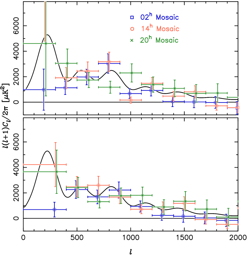
Figure 16.— Power spectrum estimates for the three CBI mosaics, treated independently. The upper panel shows the results for the odd binning, and the lower panel shows the results for the even binning. In both binnings, the lowest bin is poorly constrained by the data. In this bin, in particular, the sample variance is large. The sample variance contribution to the error estimate is a fraction of the fitted band-power, and is thus unrealistically low for the 02^h mosaic which has low fitted band-power.

Table 2Chi-Squared Comparison of the Mosaic Power Spectra

Mosaics	Binning	$\chi^{2}$ (d.o.f.)	Significance Level (per cent)
02h–14h	even	7.8 (9)	56
02h–14h	odd	5.6 (9)	78
02h–20h	even	10.3 (9)	33
02h–20h	odd	17.4 (9)	4
14h–20h	even	7.6 (9)	57
14h–20h	odd	17.5 (9)	4

4.3.3 Individual Mosaic Power Spectra

To check the consistency of the three mosaic data sets, and to look for variations in the power spectrum with direction on the sky, we have computed the power spectra of the three mosaics separately. The results are shown for the two alternate binnings in Figure 16; the very noisy points for $\ell>2000$ have been omitted. The chi-squared test (eq. [17]) shows that the 02^h and 14^h mosaics are consistent with each other, but the 20^h mosaic is discrepant at the 95% confidence level in the odd binning (see Table 2). Figure 16 shows that most of the discrepancy occurs in two adjacent bins at $700<\ell<1100$. It is unlikely that this reflects a real change in the CMB spectrum with direction, or that it could arise from, for example, foreground contamination in the 20^h mosaic, so we provisionally attribute the discrepancy to a chance statistical fluctuation. The three mosaics have galactic latitudes $-53\arcdeg$ (02^h), $48\arcdeg$ (14^h), and $-27\arcdeg$ (20^h). The good agreement between the three mosaics suggests that the CMB power spectrum is not heavily contaminated by latitude-dependent diffuse emission from the Galaxy. We will be able to examine the question of field-to-field consistency more closely when we have analyzed data from the 2001 observing season, which extend the sky coverage by a factor of two.

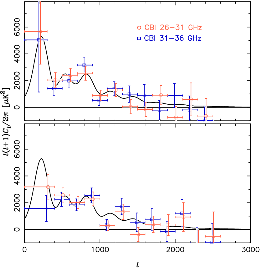
Figure 17.— Joint power spectrum estimates for the three CBI mosaics, split into the upper and lower halves of the CBI frequency band. The upper panel shows the results for the odd binning, and the lower panel shows the results for the even binning.

4.3.4 Subdivision by frequency

A second consistency check is to compare the power spectra obtained from the different CBI frequency channels. As in § 3.3, we have divided the data into low- and high-frequency halves (26–31 and 31–36 GHz). The results are shown in Figure 17. If the signal is due primarily to the CMB, the two spectra should be consistent, but if there is a large contribution from a non-thermal foreground, such as synchrotron, free-free, or dust emission, they should be different. The two spectra are similar, but it is difficult to make a quantitative comparison owing to the strong correlation between the two frequency bands. The error estimates obtained from the Fisher matrix include the contribution of cosmic variance as well as the measurement noise, so they overestimate the band-to-band variance.

5. Conclusions

The results presented in this paper demonstrate the effectiveness of interferometric mosaicing both for imaging the CMB and for measuring its power spectrum. The CBI images show for the first time structures in the CMB on mass-scales corresponding to clusters of galaxies, and the CMB power spectrum has been extended by more than a factor of two in multipole number $\ell$. Although the resolution in $\ell$ is limited (we will obtain better resolution when we analyze the wider-field observations made in 2001), we have been able to detect the second and third acoustic peaks in the spectrum, and, for the first time, the fourth and possibly the fifth. The deeper observations reported in Paper II extend the spectrum even further, well into the damping tail region where secondary anisotropies become important (see Paper VI).

Ground-based observations of the CMB in the 1-cm wave-band, where long integrations can be obtained, are competitive with balloon-based observations at shorter wavelengths. The principal obstacle to observations in this band, particularly at high $\ell$, is the emission from foreground point sources. We have shown that it is possible to correct the observations for this contamination with high accuracy, at a cost in sensitivity, but foreground sources remain the largest source of uncertainty in the power spectrum. To improve on our result, we will need sensitive high-resolution surveys of the foreground sources at 31 GHz, such as will soon be possible with the NRAO Green Bank Telescope.

It should be clear from Figures 10 and 13 that the CBI results are consistent with earlier observations in the region $\ell<1000$. What is more remarkable is that at higher $\ell$, a region that has not been probed before, the results are consistent with extrapolations of the power spectrum based on simple inflation-motivated models. We show in Paper V that the major cosmological parameters (the total density parameter, the density parameters for baryonic and non-baryonic matter, the primordial density perturbation spectral index, the Hubble constant, the cosmological constant, and the optical depth to last scattering) are well constrained by the CBI observations, even when only the region of the spectrum beyond the first two peaks is considered. This provides further strong support for cosmological models dominated by cold dark matter and dark energy, and with a scale-invariant spectrum of primordial density fluctuations up to $\ell\gtrsim 2000$. The corresponding angular scales and masses are $\sim 6^{\prime}$ and $\sim 5\times 10^{14}M_{\sun}$, the scale of galaxy clusters. This provides a firm foundation for theories of galaxy formation.

A second season of CBI mosaic observations were obtained in 2001, and are currently being analyzed. These observations double the size of each of the three mosaic fields, and will enable the power spectrum to be determined with improved sensitivity and $\ell$-resolution. We are currently reconfiguring the instrument to maximize its sensitivity to polarization, with the goal of detecting and measuring the power spectrum of the polarized component of the CMB, which is another powerful test of the cosmological models.

Table 3Summary of Observations

Field name	Date	R.A. (h, m, s)	Decl. (°, ′)	Integration time (s)
C0242$-$0230	2000 Jul 16, Oct 20	02 42 00	$-$02 30	4560
C0242$-$0250	2000 Oct 01	02 42 00	$-$02 50	7454
C0242$-$0310	2000 Jul 31, Oct 21	02 42 00	$-$03 10	4394
C0242$-$0330	2000 Oct 04, Oct 06	02 42 00	$-$03 30	14388
C0242$-$0350	2000 Aug 03, Oct 21	02 42 00	$-$03 50	5090
C0242$-$0410	2000 Oct 18	02 42 00	$-$04 10	6170
C0242$-$0430	2000 Aug 06, Oct 22	02 42 00	$-$04 30	4954
C0243$-$0230	2000 Sep 09, Oct 22, Oct 25, Oct 26	02 43 20	$-$02 30	10220
C0243$-$0250	2000 Aug 09, Oct 22	02 43 20	$-$02 50	5048
C0243$-$0310	2000 Sep 22	02 43 20	$-$03 10	6314
C0243$-$0330	2000 Aug 29	02 43 20	$-$03 30	5562
C0243$-$0350	2000 Sep 25	02 43 20	$-$03 50	5562
C0243$-$0410	2000 Sep 02	02 43 20	$-$04 10	3206
C0243$-$0430	2000 Sep 28	02 43 20	$-$04 30	7462
C0244$-$0230	2000 Oct 20	02 44 40	$-$02 30	2052
C0244$-$0250	2000 Oct 02	02 44 40	$-$02 50	7576
C0244$-$0310	2000 Aug 01, Oct 21	02 44 40	$-$03 10	4980
C0244$-$0330	2000 Oct 07	02 44 40	$-$03 30	6990
C0244$-$0350	2000 Aug 04, Oct 21	02 44 40	$-$03 50	5100
C0244$-$0410	2000 Oct 19	02 44 40	$-$04 10	3706
C0244$-$0430	2000 Aug 07, Oct 22	02 44 40	$-$04 30	5052
C0246$-$0230	2000 Sep 10	02 46 00	$-$02 30	6812
C0246$-$0250	2000 Aug 11, Aug 12	02 46 00	$-$02 50	3480
C0246$-$0310	2000 Sep 23	02 46 00	$-$03 10	6314
C0246$-$0330	2000 Aug 30, Oct 24	02 46 00	$-$03 30	9384
C0246$-$0350	2000 Sep 26	02 46 00	$-$03 50	6908
C0246$-$0410	2000 Sep 07, Oct 25, Oct 26	02 46 00	$-$04 10	13380
C0246$-$0430	2000 Sep 29	02 46 00	$-$04 30	6766
C0247$-$0230	2000 Jul 29, Oct 20	02 47 20	$-$02 30	4854
C0247$-$0250	2000 Oct 03	02 47 20	$-$02 50	7574
C0247$-$0310	2000 Aug 02, Oct 21	02 47 20	$-$03 10	5060
C0247$-$0330	2000 Oct 08	02 47 20	$-$03 30	7380
C0247$-$0350	2000 Aug 05, Oct 22	02 47 20	$-$03 50	4910
C0247$-$0410	2000 Oct 09	02 47 20	$-$04 10	2066
C0247$-$0430	2000 Aug 08, Oct 22	02 47 20	$-$04 30	5048
C0248$-$0230	2000 Sep 11, Oct 26	02 48 40	$-$02 30	8356
C0248$-$0250	2000 Aug 15, Oct 23	02 48 40	$-$02 50	9296
C0248$-$0310	2000 Sep 24	02 48 40	$-$03 10	4404
C0248$-$0330	2000 Sep 01	02 48 40	$-$03 30	5134
C0248$-$0350	2000 Sep 27, Oct 25	02 48 40	$-$03 50	5826
C0248$-$0410	$\cdots$	02 48 40	$-$04 10	$\cdots$
C0248$-$0430	2000 Sep 30	02 48 40	$-$04 30	7170
C1442$-$0230	2000 May 05	14 42 00	$-$02 30	7288
C1442$-$0250	2000 Jul 19, Aug 23	14 42 00	$-$02 50	4054
C1442$-$0310	2000 Apr 04, Apr 05, Apr 27	14 42 00	$-$03 10	26048
C1442$-$0330	2000 Jul 26, Aug 17	14 42 00	$-$03 30	4560
C1442$-$0350	2000 Mar 17, Apr 28	14 42 00	$-$03 50	14610
C1442$-$0410	2000 Aug 01, Aug 12, Aug 16	14 42 00	$-$04 10	6766
C1442$-$0430	2000 May 01	14 42 00	$-$04 30	7492
C1443$-$0230	2000 Jun 24, Aug 19	14 43 20	$-$02 30	6152
C1443$-$0250	2000 May 23	14 43 20	$-$02 50	5180
C1443$-$0310	2000 Jun 27	14 43 20	$-$03 10	6814
C1443$-$0330	2000 May 26	14 43 20	$-$03 30	5210
C1443$-$0350	2000 Jul 02	14 43 20	$-$03 50	6402
C1443$-$0410	2000 May 29	14 43 20	$-$04 10	7352
C1443$-$0430	2000 Jul 15	14 43 20	$-$04 30	5582
C1444$-$0230	2000 May 11	14 44 40	$-$02 30	8396
C1444$-$0250	2000 Jul 20, Aug 18	14 44 40	$-$02 50	5878
C1444$-$0310	2000 Apr 9, Apr 10, Apr 26	14 44 40	$-$03 10	13920
C1444$-$0330	2000 Jul 27, Aug 22	14 44 40	$-$03 30	5134
C1444$-$0350	2000 Apr 07, Apr 08, Apr 25	14 44 40	$-$03 50	13704
C1444$-$0410	2000 Jun 20, Jun 21, Jun 22	14 44 40	$-$04 10	20112
C1444$-$0430	2000 May 02	14 44 40	$-$04 30	6326
C1446$-$0230	2000 Jun 25	14 46 00	$-$02 30	5066
C1446$-$0250	2000 May 25	14 46 00	$-$02 50	5266
C1446$-$0310	$\cdots$	14 46 00	$-$03 10	$\cdots$
C1446$-$0330	2000 May 28	14 46 00	$-$03 30	4904
C1446$-$0350	2000 Jul 03	14 46 00	$-$03 50	6808
C1446$-$0410	2000 May 30	14 46 00	$-$04 10	7366
C1446$-$0430	2000 Jul 16	14 46 00	$-$04 30	4826
C1447$-$0230	2000 May 22	14 47 20	$-$02 30	7254
C1447$-$0250	2000 Jul 24, Jul 25	14 47 20	$-$02 50	4002
C1447$-$0310	2000 Apr 11, Apr 12, Apr 29	14 47 20	$-$03 10	22004
C1447$-$0330	2000 Jul 29	14 47 20	$-$03 30	4754
C1447$-$0350	2000 Apr 30, Jul 23	14 47 20	$-$03 50	8212
C1447$-$0410	2000 Aug 15, Aug 21	14 47 20	$-$04 10	5166
C1447$-$0430	2000 May 03	14 47 20	$-$04 30	4606
C1448$-$0230	2000 Jun 26	14 48 40	$-$02 30	7088
C1448$-$0250	2000 May 31	14 48 40	$-$02 50	8490
C1448$-$0310	2000 Jul 01, Aug 20	14 48 40	$-$03 10	5048
C1448$-$0330	2000 Jun 04	14 48 40	$-$03 30	6308
C1448$-$0350	2000 Jul 04	14 48 40	$-$03 50	818
C1448$-$0410	2000 Jun 07	14 48 40	$-$04 10	8058
C1448$-$0430	2000 Jul 17	14 48 40	$-$04 30	5222
C2042$-$0230	2000 Jun 04	20 42 00	$-$02 30	2844
C2042$-$0250	2000 Jul 28	20 42 00	$-$02 50	5556
C2042$-$0310	$\cdots$	20 42 00	$-$03 10	$\cdots$
C2042$-$0330	$\cdots$	20 42 00	$-$03 30	$\cdots$
C2042$-$0350	$\cdots$	20 42 00	$-$03 50	$\cdots$
C2042$-$0410	$\cdots$	20 42 00	$-$04 10	$\cdots$
C2042$-$0430	2000 May 05, Jul 02	20 42 00	$-$04 30	9392
C2043$-$0230	2000 May 31	20 43 20	$-$02 30	5930
C2043$-$0250	2000 Jun 08	20 43 20	$-$02 50	7520
C2043$-$0310	2000 Jul 05	20 43 20	$-$03 10	8024
C2043$-$0330	2000 Jun 12	20 43 20	$-$03 30	6992
C2043$-$0350	$\cdots$	20 43 20	$-$03 50	$\cdots$
C2043$-$0410	2000 Jun 26	20 43 20	$-$04 10	7128
C2043$-$0430	2000 Jul 25	20 43 20	$-$04 30	4356
C2044$-$0230	2000 May 30	20 44 40	$-$02 30	7536
C2044$-$0250	$\cdots$	20 44 40	$-$02 50	$\cdots$
C2044$-$0310	2000 May 01	20 44 40	$-$03 10	4536
C2044$-$0330	$\cdots$	20 44 40	$-$03 30	$\cdots$
C2044$-$0350	2000 May 02	20 44 40	$-$03 50	2150
C2044$-$0410	$\cdots$	20 44 40	$-$04 10	$\cdots$
C2044$-$0430	2000 May 11	20 44 40	$-$04 30	4538
C2046$-$0230	2000 Jul 03	20 46 00	$-$02 30	8724
C2046$-$0250	2000 Jun 10	20 46 00	$-$02 50	6298
C2046$-$0310	2000 Jul 06	20 46 00	$-$03 10	8722
C2046$-$0330	2000 Jun 13	20 46 00	$-$03 30	7684
C2046$-$0350	2000 Jul 23	20 46 00	$-$03 50	8302
C2046$-$0410	2000 Jun 27	20 46 00	$-$04 10	8564
C2046$-$0430	2000 Jul 26	20 46 00	$-$04 30	8260
C2047$-$0230	2000 Jun 07	20 47 20	$-$02 30	7596
C2047$-$0250	$\cdots$	20 47 20	$-$02 50	$\cdots$
C2047$-$0310	2000 May 04	20 47 20	$-$03 10	3258
C2047$-$0330	$\cdots$	20 47 20	$-$03 30	$\cdots$
C2047$-$0350	2000 May 03	20 47 20	$-$03 50	2764
C2047$-$0410	$\cdots$	20 47 20	$-$04 10	$\cdots$
C2047$-$0430	2000 May 29	20 47 20	$-$04 30	7132
C2048$-$0230	2000 Jul 04	20 48 40	$-$02 30	8312
C2048$-$0250	2000 Jun 11	20 48 40	$-$02 50	7326
C2048$-$0310	2000 Jul 07	20 48 40	$-$03 10	8652
C2048$-$0330	2000 Aug 02, Aug 23	20 48 40	$-$03 30	15316
C2048$-$0350	2000 Jul 24	20 48 40	$-$03 50	8318
C2048$-$0410	2000 Jul 01	20 48 40	$-$04 10	6660
C2048$-$0430	2000 Jul 27	20 48 40	$-$04 30	7630

References

- Bond, Jaffe, & Knox (1998) Bond, J. R., Jaffe, A. H., & Knox, L. 1998, Phys. Rev. D, 57, 2117
- Bond et al. (2003) Bond, J. R., et al. 2003, ApJ, submitted (astro-ph/0205386) (Paper VI)
- Condon et al. (1998) Condon, J. J., Cotton, W. D., Greisen, E. W., Yin, Q. F., Perley, R. A., Taylor, G. B., & Broderick, J. J. 1998, AJ, 115, 169
- Cornwell (1988) Cornwell, T. J. 1988, A&A, 202, 316
- de Bernardis et al. (2002) de Bernardis, P., et al. 2002, ApJ, 564, 559
- Halverson et al. (2002) Halverson, N. W., et al. 2002, ApJ, 568, 38
- Hobson, Lasenby, & Jones (1995) Hobson, M. P., Lasenby, A. N., & Jones, M. E. 1995, MNRAS, 275, 863
- Hobson & Maisinger (2002) Hobson, M. P., & Maisinger, K. 2002, MNRAS, 334, 569
- Knox (1999) Knox, L. 1999, Phys. Rev. D, 60, 103516
- Lee et al. (2001) Lee, A. T., et al. 2001, ApJ, 561, L1
- Maisinger, Hobson, & Lasenby (1997) Maisinger, K., Hobson, M. P., & Lasenby, A. N. 1997, MNRAS, 290, 313
- Mason et al. (1999) Mason, B. S., Leitch, E. M., Myers, S. T., Cartwright, J. K., & Readhead, A. C. S. 1999, AJ, 118, 290
- Mason et al. (2003) Mason, B. S., et al. 2003, ApJ, in press (astro-ph/0205384) (Paper II)
- Mather et al. (1999) Mather, J. C., Fixsen, D. J., Shafer, R. A., Mosier, C., & Wilkinson, D. T. 1999, ApJ, 512, 511
- Myers, Readhead, & Lawrence (1993) Myers, S. T., Readhead, A. C. S., & Lawrence, C. R. 1993, ApJ, 405, 8
- Myers et al. (2003) Myers, S. T., et al. 2003, ApJ, in press (astro-ph/0205385) (Paper IV)
- Netterfield et al. (2002) Netterfield, C. B., et al. 2002, ApJ, 571, 604
- Ng (2001) Ng, K.-W. 2001, Phys. Rev. D, 63, 123001
- Padin et al. (2000) Padin, S., Cartwright, J.K., Joy, M., & Meitzler, J.C., 2000, IEEE Trans. Antennas Propagat., 48, 836
- Padin et al. (2001) Padin, S., et al. 2001, ApJ, 549, L1 (Paper I)
- Padin et al. (2002) Padin, S., et al. 2002, PASP, 114, 83
- Sault, Staveley-Smith, & Brouw (1996) Sault, R. J., Staveley-Smith, L., & Brouw, W. N. 1996, A&AS, 120, 375
- Shepherd (1997) Shepherd, M. C. 1997, in ASP Conf. Ser. 125, Astronomical Data Analysis Software and Systems VI, ed. G. Hunt & H. E. Payne (San Francisco: ASP), 77
- Sievers et al. (2003) Sievers, J. L., et al. 2003, ApJ, in press (astro-ph/0205387) (Paper V)
- Taylor, Carilli, & Perley (1999) Taylor, G. B., Carilli, C. L., & Perley, R. A. (eds.) 1999, Synthesis Imaging in Radio Astronomy II, ASP Conf. Series 180 (San Francisco: ASP)
- Thompson, Moran, & Swenson (2001) Thompson, A. R., Moran, J. M., & Swenson, G. W., Jr. 2001, Interferometry and synthesis in radio astronomy (2nd ed.; New York: Wiley)
- White et al. (1999a) White, M., Carlstrom, J. E., Dragovan, M., & Holzapfel, W. L. 1999a, ApJ, 514, 12
- White et al. (1999b) White, M., Carlstrom, J. E., Dragovan, M., & Holzapfel, S. W. L. 1999b, preprint (astro-ph/9912422)