Dynamics and Structure of Three-Dimensional Trans-Alfvénic Jets. II. The Effect of Density and Winds

Abstract

Two three-dimensional magnetohydrodynamical simulations of strongly magnetized conical jets, one with a poloidal and one with a helical magnetic field, have been performed. In both simulations the jet is precessed at the origin to break the symmetry. The jets are denser by an order of magnitude than the jets in a previous set of simulations. Theoretical work accompanying the previous simulations indicated that an increase in jet density would stabilize the jets beyond the Alfvén point and this prediction is verified by the present simulations. In the poloidal simulation a significant sheath of magnetized moving material developed around the jet and led to additional stabilization. New theoretical work analyzing the effect of a jet embedded in a magnetized wind shows that the velocity shear, $\Delta u\equiv u_{j}-u_{e}$ must exceed a “surface” Alfvén speed, $V_{As}\equiv[(\rho_{j}+\rho_{e})(B_{j}^{2}+B_{e}^{2})/(4\pi\rho_{j}\rho_{e})]^{1/2}$, before the jet becomes unstable to helical and higher order modes of jet distortion and this explains the enhanced stability found in the poloidal simulation. The fundamental pinch mode is not similarly affected and emission knots with spacing $\sim 4R_{j}$ developed in the poloidal simulation. Thus, we identify a mechanism that can suppress large scale asymmetric structures while allowing axisymmetric structures to develop, and astrophysical jets surrounded by outflowing winds will be more stable than if surrounded by a stationary or backflowing external medium. Knotty structures along a straight protostellar jet like the jet in HH 34 or in the inner part of the jet in HH 111 could be triggered by pinching of a low magnetosonic Mach number jet surrounded by a suitable wind. Of additional interest is the development of magnetic field orientation along the line-of-sight organized by the toroidal flow field accompanying helical twisting. On astrophysical jets such structure could lead to a reversal of the direction of Faraday rotation in adjacent zones along a jet. Thus, Faraday rotation structure like that seen along the 3C 465 jet could be attributed to organized magneto-hydrodynamical structures produced by the jet flow.

1 Introduction

Jet acceleration and collimation schemes imply dynamically strong magnetic fields close to the central engine (see Meier, Koide, & Uchida 2001). Numerical studies, e.g., Meier, Payne, & Lind (1996), Ouyed, Pudritz, & Stone (1997), Ouyed & Pudritz (1997), Romanova et al. (1997), show that the jets created in this fashion pass through slow magnetosonic, Alfvénic and fast magnetosonic critical points, whose ultimate velocity may depend on the configuration of the magnetic field (Meier et al. 1997) and accelerate up to speeds that may be only a few times the Alfvén velocity at the Alfvén surface (Camenzind 1997). Thus, low magnetosonic Mach numbers might be expected for magnetically launched jets (Fendt & Camenzind 1996; Lery & Frank 2000). The numerical studies and also theoretical studies (Begelman & Blandford 1999; Lery et al. 2002) indicate that a wind or magnetized wind may surround a more rapidly moving jet.

All jet flows are susceptible to Kelvin-Helmholtz (KH) or current driven (CD) instabilities. The KH instability of 3D jets with purely poloidal or purely toroidal magnetic fields (Ray 1981; Ferrari, Trussoni, & Zaninetti 1981; Fiedler & Jones 1984; Bodo et al. 1989) and of jets containing force-free helical magnetic fields (Appl & Camenzind 1992; Appl 1996) has been extensively investigated for a stationary external medium. Additional investigations have considered the role of CD pinching of toroidally magnetized plasma columns (Begelman 1998). The CD instabilities are sensitive to the magnetic profile (Appl, Lery, & Baty 2000) and, at least for jets containing force-free helical magnetic fields, it appears that the KH instability exhibits faster growth and is more likely to be responsible for producing asymmetric structure than CD instability (Appl 1996) and CD modes appear confined to the jet interior (Appl, Lery, & Baty 2000; Lery, Baty, & Appl 2000). In general, KH growth rates increase as the magnetosonic Mach number decreases provided the jet is super-Alfvénic, but the magnetized jet is nearly completely stabilized to the KH instability when the jet is sub-Alfvénic (Hardee & Rosen 1999, hereafter Paper I). In Paper I the strongly magnetized “light” jets experienced considerable mass entrainment and slowing as denser material was entrained following destabilization. Denser jets are predicted to remain stable beyond the Alfvén point and, in general, have been found to be more robust than their less dense counterparts (Hardee, Clarke, & Rosen 1997).

In this paper we analyze results from two simulations, one with a poloidally magnetized jet and the other with a helically magnetized jet. The jets are an order of magnitude more dense than those studied in Paper I. In §2 the numerical setup and results of the numerical simulations are presented. The simulations are initialized by establishing a cylindrical helically magnetized jet across a computational grid in an unmagnetized surrounding medium with pressure gradient devised to result in an approximate constant expansion of the jet once pressure equilibrium is achieved, i.e., produce a conical jet. In one simulation a significant outwards flowing magnetized cocoon develops that influences jet stability and dynamics. This simulation shows how a jet might be influenced by a surrounding magnetized wind. Synchrotron intensity images and an integration of the line-of-sight magnetic field provide a connection between jet dynamics and observable jet emission and polarization structures. In §3 the theory is expanded to include a moving magnetized wind medium, and in §4 the predicted effect of density and winds is compared to the simulation results. Finally, in §5 we discuss some of the implications for astrophysical jets.

2 Numerical Simulations

2.1 Initialization

Simulations were performed using the three dimensional MHD code ZEUS-3D, an Eulerian finite-difference code using the Consistent Method of Characteristics (CMoC) which solves the transverse momentum transport and magnetic induction equations simultaneously and in a planar split fashion (Clarke 1996). Interpolations were carried out by a second-order accurate monotonic upwinded time-centered scheme (van Leer 1977) and a von-Neumann Richtmyer artificial viscosity was used to stabilize shocks. The code has been thoroughly tested via MHD test suites as described by Stone et al. (1992) and Clarke (1996) to establish the reliability of the techniques.

All simulations are initialized by establishing a cylindrical jet across a 3D Cartesian grid resolved into 130 $\times$ 130 $\times$ 370 zones. Thirty uniform zones span the initial jet diameter, $2R_{0}$, along the transverse Cartesian axes ($x$-axis and $y$-axis). Outside the uniform grid zones, the grid zones are ratioed where each subsequent zone increases in size by a factor 1.05. Altogether the 130 zones along the transverse Cartesian axes span a total distance of $30R_{0}$. Along the $z$-axis 280 uniform zones span a distance of $40R_{0}$ outwards from the jet origin. An additional 90 ratioed zones span an additional distance of $40R_{0}$ where each subsequent zone increases in size by a factor 1.02. The 370 zones along the $z$-axis span a total distance of $80R_{0}$. Outflow boundary conditions are used except where the jet enters the grid where inflow boundary conditions are used. The use of a non-uniform grid with larger zones at the grid boundaries has been shown to have the beneficial effect of reducing reflections off the grid boundaries as a result of increased dissipation of disturbances by the larger zone size at the grid boundaries (Bodo et al. 1995).

The jets are initialized with a uniform density $\rho_{j}$ and initial radius $R_{0}$. The magnetic field in the jet is initialized with a uniform axial component, $B_{z}$, and a toroidal magnetic component with functional form $B_{\phi}=B_{\phi}^{pk}\sin^{2}[\pi f(r)]$ where for $r<r_{pk}$, $f(r)=0.5(r/r_{pk})^{a}$, and for $r_{pk}<r<r_{\max}$, $f(r)=1.0-0.5\left[\left(1-r/r_{\max}\right)/(1-r_{pk}/r_{\max})\right]^{b}$. In these simulations the toroidal component increases to a maximum, $B_{\phi}^{pk}$, at $r_{pk}=0.5R_{0}$, and declines to zero at $r_{\max}=0.9R_{0}$ so that initially all currents flow within the jet. In the simulation with primarily axial field (simulation P), $a=1.106$ and $b=0.885$, and the FWHM of the toroidal field is $0.5R_{0}$. In the simulation with helical magnetic field (simulation T), $a=0.346$ and $b=0.277$, and the FWHM of the toroidal field is $0.8R_{0}$. These particular toroidal profiles are not physically motivated but are well behaved numerically and in simulation T the toroidal profile provides a broad cross sectional region within the jet in which the toroidal magnetic component is relatively constant (nearly constant helical pitch, plasma beta, and magnetosonic speed). In the external medium the magnetic field is equal to zero. The equation of hydromagnetic equilibrium

$$\frac{d}{dr}\left(p_{jt}(r)+\frac{B_{z}^{2}(r)}{8\pi}+\frac{B_{\phi}^{2}(r)}{8\pi}\right)=-\frac{B_{\phi}^{2}(r)}{4\pi r}\text{ ,}$$

where the term on the right hand side describes the effects of magnetic tension, has been used to establish a suitable radial gas pressure profile in the jet by varying the jet temperature. The sound, Alfvén and magnetosonic speeds are defined as $a^{2}\equiv\Gamma p/\rho$ with $\Gamma=5/3$, $V_{A}^{2}\equiv B^{2}/4\pi\rho$, and $a_{ms}^{2}\equiv a^{2}+V_{A}^{2}$. Since internal dynamics and timescales involve wave propagation across a jet with propagation speed a function of jet radius we define radial averages as, for example,

$$\left\langle M_{ms}\right\rangle\equiv\frac{1}{R_{j}}\int_{0}^{R_{j}}M_{ms}(r)dr\text{ ,}$$

that will differ for different magnetic, density, and temperature profiles.

In the simulations the external medium is isothermal and the external density $\rho_{e}(z)$ declines to produce a pressure gradient, $p_{e}(z)\propto\rho_{e}(z)$, that leads to a constant expansion, $R_{j}(z)=(1+z/80R_{0})R_{0}$, of a constant velocity adiabatic jet containing a uniform poloidal magnetic field and an internal toroidal magnetic field that provides some confinement, i.e.,

$$\rho_{e}(z)=\frac{\left[(R_{j}/R_{0})^{-10/3}+C_{p}(R_{j}/R_{0})^{-4}-C_{\phi}(R_{j}/R_{0})^{-2}\right]}{\left[1+C_{p}-C_{\phi}\right]}\rho_{e}(0)\text{ .}$$

The values of $C_{p}$ and $C_{\phi}$ depend on the poloidal and toroidal field strengths, and the ratio of the magnetic pressure relative to the thermal pressure. A pseudo-gravitational potential keeps the external medium static. Simulation P contains a primarily axial magnetic field configuration with only a weak toroidal component, $B_{\phi}^{pk}/B_{z}\sim 0.05$ at the inlet, so as to be directly comparable to predictions made by a linear stability analysis containing a $B_{z}$ magnetic field component only (§3). In simulation T, the axial magnetic field strength is identical to simulation P but now the toroidal component $B_{\phi}^{pk}/B_{z}\sim 0.44$ at the inlet. The jets are initialized with a density $\rho_{j}=0.20\rho_{e}(0)$ and with a velocity $u_{j}=1.78a_{e}$ that is trans-Alfvénic. The jet sound, Alfvén and magnetosonic speeds at jet center normalized to the external sound speed and radial averages of the jet sonic, Alfvénic and magnetosonic Mach numbers at the inlet and values of $C_{p}$ and $C_{\phi}$ for the simulations are given in Table 1. Absolute values for jet speed, density, temperature, and magnetic field strength are completely determined by choosing values for the external density, $\rho_{e}(0)$, and the external temperature, $T_{e}$, or sound speed, $a_{e}$. An absolute length scale is determined by choosing a value for $R_{0}$.

Table 1: Initial Conditions

Simulation	$u_{j}/a_{e}$	$a_{j}/a_{e}$	$V_{A,j}/a_{e}$	$a_{j}^{ms}/a_{e}$	$\left\langle M_{j}\right\rangle$	$\left\langle M^{A}_{j}\right\rangle$	$\left\langle M^{ms}_{j}\right\rangle$	$C_{p}$	$C_{\phi}$
P	1.78	1.32	1.90	2.31	1.43	0.89	0.75	1.721	0.005
T	1.78	1.41	1.90	2.37	1.26	0.87	0.70	1.506	0.294

In both simulations the jet is driven by a periodic precession of the jet velocity, $u_{j}$, at an angle of 0.01 radian relative to the $z$-axis with an angular frequency $\omega=0.5a_{e}/R_{0}$. The initial transverse motion imparted to the jet by this precession is well within the linear regime. The precession serves to break the symmetry and the precessional frequency is chosen to be below the theoretically predicted maximally unstable frequency associated with helical twisting of a KH unstable supermagnetosonic jet with jet radius $R_{j}\geq R_{0}$. In both simulations the precession is in a counterclockwise sense when viewed outwards from the inlet. This direction of precession induces a helical twist in the same sense as that of the magnetic field helicity.

In both simulations the jets expand rapidly and after about five dynamical times, $\tau_{d}\equiv(a_{e}/R_{0})t\approx 5$, have achieved an approximate static pressure equilibrium with the surrounding medium, and a nearly constant expansion rate on the computational grid with $R_{j}\approx 2R_{0}$ when $z=80R_{0}$.

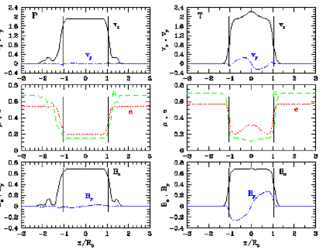
Figure 1: Profiles (along the $x$-axis) of axial and azimuthal velocity, $v_{z}$ & $v_{y}$, respectively, density and internal energy, $\rho$ & $e$, and magnetic field components, $B_{z}$ & $B_{y}$ for simulations P (left) and T (right) at $z/R_{0}=4.5$. The vertical lines indicate the location of a conical jet‘s surface at this distance from the inlet.

The code modifies the initial input static equilibrium state to an appropriate dynamic equilibrium state, i.e., $\nabla\times({\mathbf{u}}\times{\mathbf{B}})=0$ throughout the duration of the simulation within an axial distance of one jet radius from the inlet. Velocity, density, internal energy and magnetic field profiles representative of the initial dynamic equilibrium in the two simulations are shown in Figure 1.

The simulations were terminated at dynamical times (P) $\tau_{d}\equiv(a_{e}/R_{0})t=96$ and (T) $\tau_{d}\equiv(a_{e}/R_{0})t=56$ when computational difficulties arose. At these times the simulations have reached a quasi-steady state out to axial distances of about (P) $60R_{0}$ and (T) $35R_{0}$. At this time the jet had undergone (P) $\sim 21.4$ and (T) $\sim 12.5$ precessional periods and (P) $\sim 3.7$ and (T) $\sim 2.2$ flow through times, $\tau_{fl}\equiv(z/u)(a_{e}/R_{0})$, through $z=50R_{0}$. Typically a quasi-steady state is achieved after 3 flow through times at a particular distance. Each simulation required roughly 110 CPU hours on the Cray T90 at the San Diego Supercomputer Center.

2.2 Simulation Results

2.2.1 Jet Structure

Plots of the total pressure, $p^{*}\equiv p_{th}+p_{bz}$, normalized by the external pressure p_e and velocity components along 1D cuts parallel to the jet axis in the $x$-$z$ slice plane are shown in Figure 2.

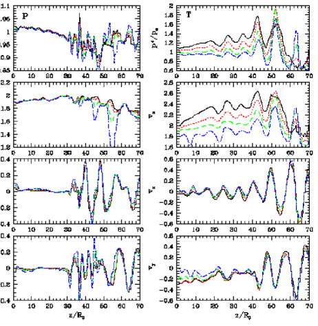
Figure 2: Cuts in the $x$-$z$ plane parallel to the $z$-axis at $x/R_{0}=$ (solid line) 0.233, (dotted line) 0.433, (dashed line) 0.633, (dot-dash line) 0.833 of jet total pressure, $p^{*}$, normalized by the external thermal pressure, $p_{e}$, and the three velocity components normalized by the external sound speed, $a_{e}$, for simulations P (left) and T (right).

In this slice plane $v_{x}$ and $v_{y}$ correspond to a radial velocity, $v_{r}$, and an azimuthal velocity, $v_{\phi}$, respectively, provided the jet center is not displaced off the $z$-axis. The jet accelerates in response to thermal and magnetic pressure gradients, and to the pseudo-gravitational potential. In simulation P with primarily poloidal magnetic field the jet accelerates to 5% above the value at the inlet. In simulation T additional acceleration occurs, to about 20% above the inlet value, as a result of the “spring” effect from the helical magnetic field. Instability is most obviously manifested by the oscillations and growth in the amplitude of the transverse velocity components, but also appears in total pressure and axial velocity fluctuations. Low level fluctuations in $p^{*}$ and $v_{z}$ appear in both simulations by $z\sim 5R_{0}$. Significant fluctuations do not begin to grow until $z\sim 30R_{0}$ in simulation P, but become significant by $z\sim 15R_{0}$ in simulation T.

In simulation P we can identify the following features:

1. At $z/R_{0}<30$ a short wavelength, $\lambda\lesssim 5R_{0}$, low amplitude oscillation in $p^{*}$ (also in $v_{z}$ but only one oscillation obvious with the velocity scale used in the figure).

2. At $30<z/R_{0}<50$ a region of rapid growth and complex structure, showing rapid oscillations in $v_{y}$ ($v_{\phi}$) and a dominant oscillation in $v_{x}$ ($v_{r}$) with $\lambda\lesssim 8R_{0}$.

3. At $z>55R_{0}$ dominant out of phase transverse velocity oscillations indicative of helical twisting with $\lambda\sim 10R_{0}$ moving with $v_{w}\sim 0.75a_{e}\sim 0.40u_{j}$ where $u_{j}\sim 1.9a_{e}$ (v_w determined from sequential simulation frames).

In simulation T we can identify the following features:

1. At $z<40R_{0}$ a region with growing amplitude oscillations in $p^{*}$, $v_{z}$ and $v_{x}$ with $\lambda\lesssim 8R_{0}$.

2. At $z>40R_{0}$ dominant out of phase transverse velocity oscillations indicative of helical twisting with $\lambda\sim 10R_{0}$ moving with $v_{w}\sim 0.91a_{e}\sim 0.41u_{j}$ where $u_{j}\sim 2.2a_{e}$.

Plots of the axial velocity along with the sonic, Alfvénic and magnetosonic speeds along 1D cuts parallel to the jet axis in the $x$-$z$ slice plane inside and outside the jet are shown in Figure 3.

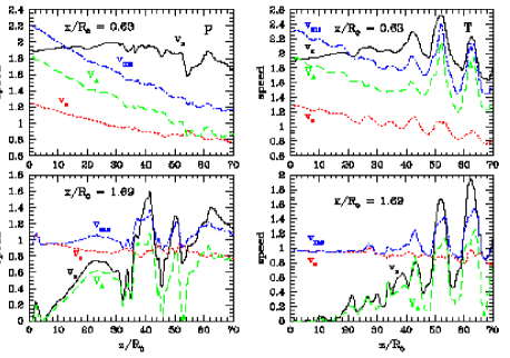
Figure 3: Cuts in the $x-z$ plane parallel to the $z$-axis inside the jet (top) and outside the jet (bottom) in simulations P (left) and T (right) showing the (solid line) axial flow speed, $v_{z}$, the (dot-dash line) magnetosonic speed, $v_{ms}$, the (dashed line) Alfvén speed, $V_{A}$, and the (dotted line) sound speed, $v_{s}$.

The cut at $x/R_{0}=1.69$ contacts the conical jet’s “surface” at $z=55R_{0}$ but adequately represents conditions immediately outside the jet at $z<40R_{0}$. The cut inside the jet shows that, in both simulations, the jets are super-Alfvénic just outside the inlet and are super-magnetosonic by $z=20R_{0}$. The cut outside the jet reveals that a significant boundary layer forms outside the jet in simulation P by $z=15R_{0}$ with flow and Alfvén speeds almost half their values inside the jet.

The differences in transverse structure in the simulations is shown by velocity, density, internal energy and magnetic field profiles at $z=18R_{0}$ shown in Figure 4. In both simulations the boundary layer has a thickness greater than $0.5R_{0}$ but only in simulation P is there significant flow and magnetic field in the boundary layer.

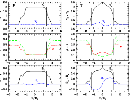
Figure 4: Profiles (along the $x$-axis) of axial and azimuthal velocity, $v_{z}$ & $v_{y}$, respectively, density and internal energy, $\rho$ & $e$, and magnetic field components, $B_{z}$ & $B_{y}$ for simulations P (left) and T (right)at $z/R_{0}=18.0$. The vertical lines indicate the location of a conical jet‘s surface at this distance from the inlet.

2.2.2 Mass Entrainment

The mass entrained by the jets and the average velocity of jet plus entrained material in the two simulations is plotted in Figure 5. In particular, we define the mass per unit length, $\sigma(z)$, at any point along the jet as $\sigma=\int_{A}f\rho dydx$, where A is the cross sectional area of the computational domain at axial position $z$, and $f$ is set to 1 if the local magnetic field is above 4% of the expected maximum field strength along the jet at $z$ [$B(z)>0.04B_{j,max}(z)$] and $f$ is set to 0 otherwise. We define the entrained mass by the presence of a magnetic field since only the jet material is initially magnetized. The setting of $f$ to 1 or 0 effectively assumes that zones with a fraction of jet material, as defined by the presence of magnetic field, are considered mixed with the external medium in that zone. While one may expect that flux-freezing will prevent the magnetized mass from increasing along the grid, here the jets are unstable. Vorticies at the jet’s surface lead to intertwining of filaments or sheets of jet and external material, and numerical diffusion leads to mixing. This technique provides results similar to estimating mass entrainment by using an axial velocity threshold (Rosen, Hardee, Clarke, & Johnson 1999; hereafter RHCJ). Setting the switch at a magnetic field strength of 4% of the expected maximum strength at $z$ reduces the sensitivity of the value of $\sigma$ to a small numerical diffusion of the field into the denser “unmixed” external medium.

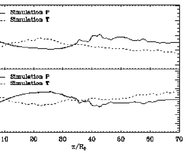
Figure 5: Profiles of the total magnetized mass (jet plus entrained material) per unit length, $\sigma(z)$, and of the average speed of magnetized jet plus entrained material.

In the very light jet simulations presented in paper I, there was a large increase in $\sigma$ near the jet inlet and $\sigma/\sigma_{jet}=10$ ($\sigma_{jet}$ is the expected value at the inlet) was used as a baseline value. In these denser jet simulations some immediate increase is observed but now $\sigma/\sigma_{jet}\sim 2.5$ serves as an appropriate baseline value. In simulation P an increase in $\sigma/\sigma_{jet}$ and a decrease in $\langle v_{z}\rangle/a_{e}$ at $z\sim 30R_{0}$ reflects the point at which significant velocity and pressure fluctuations appear. Simulation T shows a small increase in $\sigma/\sigma_{jet}$ and a decrease in $\langle v_{z}\rangle/a_{e}$ at $z\sim 10R_{0}$ coincident with growth of significant velocity and pressure fluctuations.

The maximum value of the mass per unit length is $(\sigma/\sigma_{jet})^{\mathrm{m}ax}\approx$ (P) 4 and (T) 3.5. These values imply a jet plus entrained mass of about (P) 1.6 and (T) 1.4 times the initial baseline mass per unit length. The mass entrained in simulation P is similar to the poloidally magnetized simulation B in paper I. The mass entrained in simulation T is roughly half that in the toroidal simulations C & D in paper I, but this difference is attributable to the early termination of simulation T before a quasi-steady state could be achieved at large $z$, e.g., note the decline in the jet plus entrained mass at larger axial distances. While the effect of mass entrainment on the jets here is somewhat reduced relative to the “light” jets studied in paper I, we again find that significant mass entrainment does not occur until the jets destabilize.

The average axial velocity of magnetized material indicates that the entrained material is moving more rapidly than was found in the light jet simulations in paper I. This result indicates that a denser jet is capable of accelerating entrained material to higher velocities. In simulation P we note that the average axial velocity of magnetized material increases significantly to a maximum at $z/R_{0}\sim 25$ while at the same time $\sigma/\sigma_{jet}$ decreases to a minimum. This behavior is coincident with the formation of a significant sheath of magnetized material moving at up to 38% of the jet speed (see Figure 3 for velocities in the sheath). In both simulations the majority of the momentum flux, $\sigma v_{z}^{2}$, [(P) 98% and (T) 92%] evaluated within the quasi-steady state region of the computational grid is carried by jet plus entrained material, i.e., material with $B(z)>0.04B_{j,max}(z)$.

2.2.3 Velocity, Emission & Magnetic Field Images

Jet axial velocity cross sections shown in Figure 6 illustrate development of the surface distortions that promote mixing and mass entrainment, and the large scale distortions that can move the jet flow completely off the initial axis.

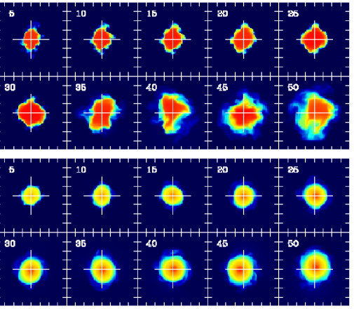
Figure 6: Jet velocity cross sections at axial distances indicated in the panels for simulation P (top 10 panels) and simulation T (bottom ten panels). The number in the upper left corner of each panel indicates distance from the inlet in units of $R_{0}$.

In simulation P small scale surface corrugations form before the jet becomes grossly unstable. A similar result was obtained in paper I for “light” poloidally magnetized jets. An elliptical distortion of the jet cross section is evident in the panels at $z/R_{0}=30$ & $35$, and considerable cross section distortions and displacement of the jet off the initial axis occur at larger $z$. In simulation T the jet exhibits much reduced distortion and the higher order surface corrugations that appear in simulation P at $z<35R_{0}$ are suppressed. These results are similar to what was found in paper I. An elliptical distortion is evident in the panels $z/R_{0}=10-30$ and the jet is displaced off the initial axis for $z>25R_{0}$.

Synchrotron intensity images and images of an integration of the magnetic field component, $B_{y}$, along the line-of-sight are shown in Figures 7 & 8. To some extent these images also reveal the extent of jet spreading as only the jet fluid is magnetized. To generate the synchrotron intensity images a synchrotron emissivity is defined by $p_{j}(B\sin\theta)^{3/2}$ where $\theta$ is the angle made by the magnetic field with respect to the line of sight. This emissivity mimics synchrotron emission from a system in which the energy and number densities of the relativistic particles are proportional to the energy and number densities of the thermal fluid. This simplistic assumption is necessary when the relativistic particles are not explicitly tracked (Clarke, Norman, & Burns 1989).

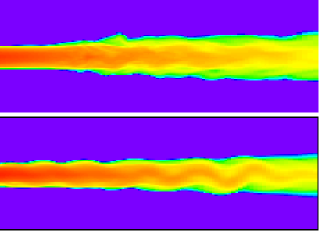
Figure 7: Synchrotron intensity images in the $x$-$z$ plane from line-of-sight integrations through the computational domain along the $y$-axis. Image dimensions are $20R_{0}\times 80R_{0}$ and the logarithmic scale spans six orders of magnitude. Simulations P and T are top and bottom images, respectively.

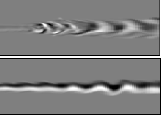
Figure 8: Integration showing the line-of-sight direction of the magnetic field ($B_{y}$) in simulations P (top) and T (bottom). Image dimensions are identical to Figure 7.

The line-of-sight magnetic field changes direction in adjacent bands in simulation P. The effect is most pronounced at larger $z$ where a pronounced helical twist has developed in the jet flow. The poloidal magnetic field is organized by the toroidal flow field accompanying the helical twist. The line-of-sight magnetic image for simulation T reflects the orientation of the initial toroidal field component. In simulation T the toroidal magnetic field is too strong to be overcome by reorientation of the poloidal field by the toroidal flow field accompanying the helical twist.

2.2.4 Pinch Structure at Intermediate Time

At dynamical times $\tau_{d}\sim 39$ the simulations have not yet developed strong asymmetries. In Figure 9 synchrotron intensity images, containing fractional polarization B-vectors formed from the Stokes parameters, reveal observational structures that develop on the trans-Alfvénic jets at intermediate times.

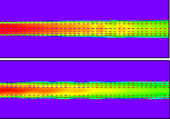
Figure 9: Synchrotron intensity images in the $x$-$z$ plane from line-of-sight integrations through the computational domain along the $y$-axis. Vectors indicate apparent magnetic field direction. Image dimensions are $10R_{0}\times 40R_{0}$ and simulations P and T are top and bottom images, respectively.

Axisymmetric intensity knots appear contained within the jet interior in simulation P and are closely spaced. Intensity knots do not appear in simulation T and the development of sinusoidal oscillation is already apparent in the jet interior. In simulation P the emission knots, visible in Figure 9 between $25<z/R_{0}<35$, have spacing $\lambda\lesssim 4R_{0}$ and move with $v_{w}\sim 0.85a_{e}\sim 0.45u_{j}$ where $u_{j}\sim 1.9a_{e}$. It is interesting that the emission knots appear in simulation P containing only a very weak toroidal field component. In simulation T the stronger toroidal field component might have been expected to be more conducive to knot formation via a pinch instability. We will show that the presence of flow outside the jet in simulation P has suppressed asymmetric structures and allowed the knots to form.

3 Theoretical Analysis

3.1 Stability Theory

Let us model the jet as a cylinder of radius $R_{j}$, having a uniform density, $\rho_{j}$, a uniform internal axial magnetic field, B_j, and a uniform velocity, u_j. The external medium is assumed to have a uniform density, $\rho_{e}$, a uniform external axial magnetic field, B_e, and a uniform velocity, u_e. The jet is established in static total pressure balance with the external medium where the total static pressure is $p_{j}^{*}\equiv p_{j}+B_{j}^{2}/8\pi=$ $p_{e}^{*}=p_{e}+B_{e}^{2}/8\pi$. Inclusion of a small non-uniform toroidal magnetic field component like that used in simulation P will not significantly modify results obtained from a linear analysis involving small fluctuations incorporating only axial magnetic fields, although we expect significant effects associated with the much stronger toroidal magnetic field used in simulation T, e.g., Appl & Camenzind (1992), Appl (1996), Rosen et al. (1999). The general approach to analyzing the stability properties of this system is to linearize the one-fluid MHD equations of continuity and momentum along with an equation of state where the density, velocity, pressure, and magnetic field are written as $\rho=\rho_{0}+\rho_{1}$, ${\mathbf{u}}={\mathbf{u}}_{0}+{\mathbf{u}}_{1\text{,}}$ $p=p_{0}+p_{1}$, ${\mathbf{B}}={\mathbf{B}}_{0}+{\mathbf{B}}_{1}$, and subscript 1 refers to a perturbation to the equilibrium quantity. Axial magnetic fields in cylindrical geometry have been investigated in several articles (Ray 1981; Ferrari, Trussoni, & Zaninetti 1981; Fiedler & Jones 1984; Bodo et al. 1989) although in general it has been assumed that there is no flow in the external medium. The relatively slow jet expansion in the numerical simulations is not expected to significantly modify local results based on a completely uniform external medium (Hardee 1984).

In cylindrical geometry a random perturbation of $\rho_{1}$, ${\mathbf{u}}_{1\text{,}}$ $p_{1}$, and ${\mathbf{B}}_{1}$ to an initial equilibrium state $\rho_{0}$, ${\mathbf{u}}_{0\text{, }}$ $p_{0}$, and ${\mathbf{B}}_{0}$ can be considered to consist of Fourier components of the form

$$f_{1}(r,\phi,z)=f_{1}(r)\exp[i(kz\pm n\phi-\omega t)]\text{ ,}$$ (1)

where the flow is along the $z$-axis, and $r$ is in the radial direction with the flow bounded by $r=R_{j}$. In cylindrical geometry $k$ is the longitudinal wavenumber, $n$ is an integer azimuthal wavenumber, for $n>0$ the wavefronts are at an angle to the flow direction, the angle of the wavevector relative to the flow direction is $\theta=\tan(n/kR_{j})$, and $+n$ and $-n$ refer to wave propagation in the clockwise and counterclockwise sense, respectively, when viewed outwards along the flow direction. In equation (1) $n=$ 0, 1, 2, 3, 4, etc. correspond to pinching, helical, elliptical, triangular, rectangular, etc. normal mode distortions of the jet, respectively. Propagation and growth or damping of the Fourier components is described by the dispersion relation

$$\frac{\beta_{j}}{\chi_{j}}\frac{J_{\pm n}^{{}^{\prime}}(\beta_{j}R)}{J_{\pm n}(\beta_{j}R)}=\frac{\beta_{e}}{\chi_{e}}\frac{H_{\pm n}^{(1)^{\prime}}(\beta_{e}R)}{H_{\pm n}^{(1)}(\beta_{e}R)}\text{ ,}$$ (2)

where $J_{\pm n}$ and $H_{\pm n}^{(1)}$ are Bessel and Hankel functions, the primes denote derivatives of the Bessel and Hankel functions with respect to their arguments, and we have dropped the subscript on the jet radius, i.e., $R\equiv R_{j}$. In equation (2)

$$\beta_{j}=\left[-k^{2}+\frac{(\omega-ku_{j})^{4}}{(\omega-ku_{j})^{2}(a_{j}^{2}+V_{Aj}^{2})-k^{2}V_{Aj}^{2}a_{j}^{2}}\right]^{1/2}\text{, }\beta_{e}=\left[-k^{2}+\frac{(\omega-ku_{e})^{4}}{(\omega-ku_{e})^{2}(a_{e}^{2}+V_{Ae}^{2})-k^{2}V_{Ae}^{2}a_{e}^{2}}\right]^{1/2}\text{ ,}$$

and

$$\chi_{j}=\rho_{j}[(\omega-ku_{j})^{2}-k^{2}V_{Aj}^{2}]\text{ , }\chi_{e}=\rho_{e}[(\omega-ku_{e})^{2}-k^{2}V_{Ae}^{2}]\text{ ,}$$

where $u_{j,e}$, $a_{j,e}$ and $V_{Aj,e}$ are the flow, sound and Alfvén speeds in the appropriate medium.

In general, each normal mode, $n$, contains a single “surface” wave and multiple “body” wave solutions that satisfy the dispersion relation. The behavior of the solutions can be investigated analytically and we extend previous analytical 3D results here to include for the possibility of an external medium with axial magnetic field and flow.

3.2 Analytical Approximations

The $n=0$ pinch mode “fundamental” (not a surface wave in this case) wave solution can be found from the dispersion relation in the low frequency limit $\omega\rightarrow 0$ and $k\rightarrow 0$. In this limit $\beta_{j}R\rightarrow 0$, $\beta_{e}R\rightarrow 0$ and the dispersion relation becomes

$$\chi_{j}\approx-\chi_{e}(\beta_{j}R)^{2}[ln(\beta_{e}R)-i\pi/2]/2\text{ ,}$$

where we have used $[J_{0}^{{}^{\prime}}(\beta_{j}R)]/[J_{0}(\beta_{j}R)]\rightarrow-\beta_{j}R/2$ and $[H_{0}^{(1)}(\beta_{e}R)]/[H_{0}^{(1)^{\prime}}(\beta_{e}R)]\rightarrow(\beta_{e}R)[ln(\beta_{e}R)-i\pi/2]$. As $(kR)^{2}\rightarrow 0$ faster than $ln(\beta_{e}R)\rightarrow-\infty$, the real part of the solution to the dispersion relation remains nearly unmodified by the presence of a magnetized wind around the jet and is given by (Paper I)

$$\frac{\omega}{k}\approx u_{j}\pm\left\{\frac{1}{2}\left(V_{Aj}^{2}+\frac{V_{Aj}^{2}a_{j}^{2}}{a_{msj}^{2}}\right)\pm\frac{1}{2}\left[\left(V_{Aj}^{2}+\frac{V_{Aj}^{2}a_{j}^{2}}{a_{msj}^{2}}\right)^{2}-4\frac{V_{Aj}^{4}a_{j}^{2}}{a_{msj}^{2}}\right]^{1/2}\right\}^{1/2}\text{ ,}$$ (3)

where $a_{msj}\equiv\left(a_{j}^{2}+V_{Aj}^{2}\right)^{1/2}$is the magnetosonic speed. The imaginary part of the solution is vanishingly small in the low frequency limit. These solutions are related to fast ($+$) and slow ($-$) magnetosonic waves propagating with ($u_{j}+$) and against ($u_{j}-$) the jet flow speed $u_{j}$, but modified by the jet-external medium interface. The unstable growing solution is associated with the backwards moving (in the jet fluid reference frame) slow magnetosonic wave. The growth rate can only be determined by numerical solution of the dispersion relation.

The $n>0$ higher order mode “surface” wave solutions can also be found from the dispersion relation in the low frequency limit. In this case the dispersion relation becomes

$$\chi_{j}\approx-\chi_{e}\text{ ,}$$

where we have used $[J_{\pm n}^{{}^{\prime}}(\beta_{j}R)H_{\pm n}^{(1)}(\beta_{e}R)]/[J_{\pm n}(\beta_{j}R)H_{\pm n}^{(1)^{\prime}}(\beta_{e}R)]\rightarrow-(\beta_{e}R)/(\beta_{j}R)$. The solution is modified by the presence of a magnetized wind around the jet and is given by

$$\frac{\omega}{k}=\frac{u_{e}+\eta u_{j}}{1+\eta}\pm i\frac{\eta^{1/2}}{1+\eta}\left[(u_{j}-u_{e})^{2}-V_{As}^{2}\right]^{1/2}\text{ ,}$$ (4)

where $\eta\equiv\rho_{j}/\rho_{e}$ and $V_{As}^{2}\equiv(\rho_{j}+\rho_{e})(B_{j}^{2}+B_{e}^{2})/(4\pi\rho_{j}\rho_{e})$. Growth corresponds to the plus sign in equation (4), but these higher order surface modes are predicted to be stable when $(u_{j}-u_{e})^{2}-V_{As}^{2}<0$. When there is no flow and no axial magnetic field outside the jet, equation (4) reduces to equation (4a) in Paper I. In this case the stability condition can be written as $u_{j}^{2}-(1+\eta)V_{Aj}^{2}<0$. These surface modes are strongly influenced by flow and magnetic field in the medium outside the jet. In the dense jet limit, i.e., $\eta\rightarrow\infty$ and $V_{As}^{2}\rightarrow\eta V_{Aj}^{2}$, equation (4) becomes $\omega/k\approx u_{j}\pm V_{Aj}$. The present reanalysis in this limit reveals an error in paper I where we stated incorrectly that $\omega/k\approx u_{j}\pm V_{Aj}$ applied when the jet was sub-Alfvénic and stable independent of the jet density. The unstable growing solution is associated with the backwards moving (in the jet fluid reference frame) Alfvén wave. When a jet is trans-magnetosonic and trans-Alfvénic the growth (damping) rates of these wave modes can only be determined by numerical solution of the dispersion relation.

The “body” wave solutions are somewhat modified by the presence of a magnetized wind surrounding a jet and in the limit $\omega\rightarrow 0$ and $k\neq 0$ the dispersion relation becomes

$$\beta_{j}R-n\pi/2-\pi/4\approx\pm\frac{\pi}{2}\left[1-C_{n}\right]\text{ ,}$$

where we have used $J_{n}(z)\approx(2/\pi z)^{1/2}cos(z-n\pi/2-\pi/4)$, $\theta=cos^{-1}\epsilon\approx\pi/2-\epsilon$, and $C_{n}<<1$ is a correction term given by

$$C_{n}=\frac{2}{\pi}\frac{\chi_{e}}{\chi_{j}}\frac{\beta_{j}}{\beta_{e}}\frac{H_{n}^{(1)}(\beta_{e}R)}{H_{n}^{(1)^{\prime}}(\beta_{e}R)}\left(\frac{\pi\beta_{j}R}{2}\right)^{1/2}J_{n}^{{}^{\prime}}(\beta_{j}R)\text{ .}$$

The solutions are given by

$$kR\approx\frac{(n+2m+1/2)\pi/2-\pi/2(1-C_{n})}{\left[\{M_{msj}^{2}/[1-(M_{msj}/M_{j}M_{Aj})^{2}]\}-1\right]^{1/2}}\text{ ,}$$ (5)

where $m\geq 1$ is an integer When the external medium is unmagnetized and there is no wind $\chi_{e}|_{\omega=0}=\rho_{e}[u_{e}{}^{2}-V_{Ae}^{2}]k^{2}=0$ and $C_{n}=0$. Previously we found that unstable body wave solutions exist only when the denominator in equation (5) is real and that body mode growth rates, with the exception of the 1st pinch body mode, remain small unless the jet is sufficiently supermagnetosonic. Thus, we do not expect to find structure attributable to higher order, $n>0$, body modes in the present simulations.

3.3 Numerical Solutions

We have investigated the effects of external magnetic fields and winds on jet stability by solving the dispersion relation numerically using root finding techniques. The analytical expressions provide an initial estimate for solutions in the low frequency limit. We have considered a set of parameters relevant to numerical simulations P & T at a distance $z\sim 18R_{0}$ from the inlet. These parameters are given in Table 2.

Table 2: Parameters at $z\sim 18R_{0}$

Simulation	$\eta$	$u_{j}/a_{e}^{ms}$	$u_{e}/a_{e}^{ms}$	$M_{j}$	$M^{A}_{j}$	$M^{ms}_{j}$	$p_{j}/p^{*}_{j}$	$p_{e}/p^{*}_{e}$
P	0.3	2.20	0.77	2.23	1.43	1.20	0.33	0.80
T	0.3	2.20	0.00	2.23	1.43	1.20	0.33	1.00

Solutions to the dispersion relation can be sensitive to the wind speed and to the presence or absence of a magnetic field in the wind/external medium. Solutions that are growing in one parameter regime can be damped in another parameter regime. Thus, we have computed and show both growing and damped solutions to the dispersion relation for an unmagnetized and a magnetized wind at wind speeds from zero up to those observed in simulation P. The root finding techniques were not always capable of converging to a solution at all frequencies or of finding a solution unless a very accurate initial estimate could be supplied. Solutions generally consist of a growing and damped pair of roots and it was not always possible to find both solutions; e.g., the root finder would not converge to the damped fundamental pinch mode solution associated with the outwards moving (in the jet fluid reference frame) slow magnetosonic wave. Not all of the possible solutions are shown. For example, the fast magnetosonic wave solutions associated with the fundamental pinch mode are not included and various additional “wind” associated solutions found in the numerical investigation are also not shown. In general, these additional solutions are purely real or damped, and will not affect the stability properties of the jet.

3.3.1 The Fundamental Pinch and Asymmetric Surface Modes

In the absence of a magnetic field in the external environment the behavior of solutions to the dispersion relation is shown for a representative sample of wind speeds in Figure 10. Solutions corresponding to the ‘backwards’ moving waves (in the jet fluid frame) are shown in the leftmost panels and solutions corresponding to the ‘forwards’ moving waves (in the jet fluid frame) are shown in the rightmost panels. The wind speeds are indicated in the panels in units of the magnetosonic speed in the external medium, in this case equal to the sound speed in the external medium. The panels for an unmagnetized external medium with no external wind are indicative of the expected stability properties of the jet in simulation T. In simulation T there is little wind or magnetic field external to the jet, i.e., $u_{e}=0$ and $p_{e}/p^{*}_{e}=1$. The higher order ($n>1$) surface modes grow much faster than the pinch fundamental mode and would be expected to dominate the dynamics.

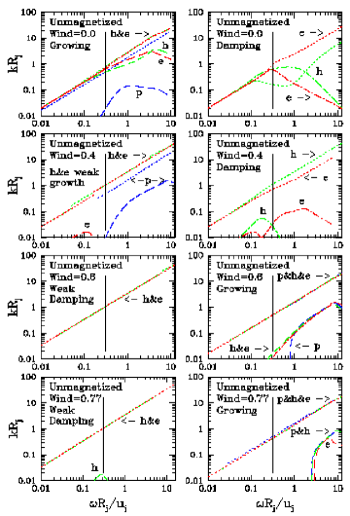
Figure 10: Solutions to the dispersion relation for surface pinch (p), helical (h), and elliptical (e) wave modes. Dotted lines indicate the real part of the wavenumber. Dashed (growing) and dash-dot (damping) lines indicate the imaginary part of the wavenumber. The vertical line indicates the location of the precession frequency used in the simulations but normalized to the jet radius and velocity at $z=18R_{0}$. In the panels the wind speed is indicated in units of $a_{e}^{ms}$.

As the wind speed is increased the growth (damping) rates of helical and higher order surface modes are, at first, greatly decreased as predicted analytically by equation (4) at low frequencies (compare the top two rows of panels in Figure 10). For these lower wind speeds growth of the fundamental pinch mode is enhanced by the presence of an external wind and can greatly exceed that of the helical and higher order asymmetric modes. There is a relatively abrupt change in behavior of the solutions when the wind speed is about 50% of the sound speed in the external medium. At lower wind speeds the ‘backwards’ moving waves are growing and the ‘forwards’ moving waves are damped. At higher wind speeds the ‘forwards’ moving helical and higher order surface modes move with speed comparable to the fundamental pinch mode and are growing, and the ‘backwards’ moving waves are damped. At these higher wind speeds growth of the pinch and higher order modes are comparable and relatively large, albeit at high frequencies only. However, as the wind speed increases further all growth rates diminish. In general, growth of the higher order modes is suppressed as the result of an external wind.

The solutions to the dispersion relation are very sensitive to a magnetized wind and this sensitivity to relatively low speed magnetized winds is shown in Figure 11.

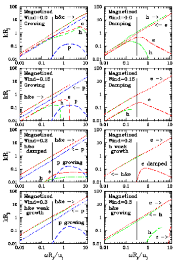
Figure 11: Surface mode solutions to the dispersion relation for a magnetized external medium at lower wind speeds. Notation is identical to that of Figure 10.

As in Figure 10 solutions corresponding to the ‘backwards’ and ‘forwards’ moving waves (in the jet fluid frame) are shown in the left and right columns, respectively. Here the external magnetic field has a value similar to that seen in simulation P. Note that the external magnetic field has a minimal effect on the growth rates in the absence of a wind (compare the top left panel in Figure 11 with the top left panel in Figure 10). Comparison between the leftmost panels in the top and second row in Figure 11 shows a reduction in helical and elliptical growth rates at low frequencies predicted analytically by equation (4). In general, increase in the wind speed stabilizes the higher order surface modes at the lower frequencies while leaving the fundamental pinch mode growth rate unchanged. However, when the ‘forwards’ moving helical and higher order surface modes move with speed comparable to the fundamental pinch mode they are growing and the maximum growth rate of the pinch and higher order modes is again comparable (see the bottom panels in Figure 11), albeit growth of the higher order modes is restricted to high frequencies. We note here that we do not confirm the result for the wave speed of the higher order surface modes in the stable region as was stated in paper I. The wave speed is given properly by equation (4) in this paper with the previously stated result, $v_{w}\approx u_{j}+V_{Aj}$, only appropriate in the dense jet limit. The error in paper I resulted from an apparent but not true convergence of the root finding routine.

There is a relatively abrupt break point in behavior of the solutions when the magnetized wind speed is about 35% of the magnetosonic speed in the external medium, and solutions at higher magnetized wind speeds are shown in Figure 12.

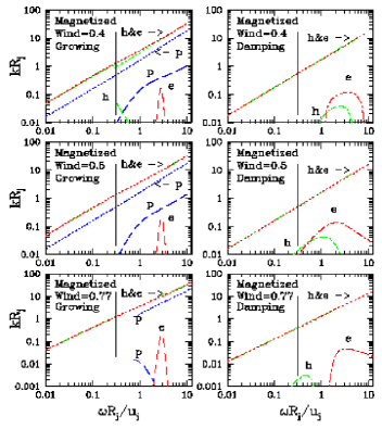
Figure 12: Surface mode solutions to the dispersion relation for a magnetized external medium at higher wind speeds. Notation is identical to that of Figures 10 & 11. Note the different vertical scale in the bottom two panels (required to show the greatly reduced growth and damping rates).

Once again the ‘backwards’ and ‘forwards’ moving solutions are shown in the left and right columns, respectively. In general, higher order surface mode growth rates are significantly reduced by these higher speed magnetized winds. In these magnetized wind cases our root finding techniques were unable to converge to solutions at lower frequencies for the pinch fundamental mode at the highest wind speed and in an intermediate frequency range where we assume that the helical surface mode will exhibit a narrow instability range similar to that exhibited by the elliptical surface mode. Nevertheless, with the exception of the highest wind speeds the fundamental pinch mode is the most unstable and should dominate the dynamics. The computations in the bottom two panels indicate that the magnetized wind observed in simulation P at the termination of the simulation reduces the growth rate of the pinch mode by about an order of magnitude, and restricts growth of the higher order surface modes to a very narrow frequency range. Clearly the fast magnetized wind in simulation P is responsible for the stability of the jet to far beyond the Alfvén point.

3.3.2 The Body Modes

The analytical approximations at low frequency indicate that the real part of the body mode solutions will be only minimally modified by the presence of an external magnetic field or wind. The extent to which a wind modifies the growth rates at higher frequencies is shown in Figure 13.

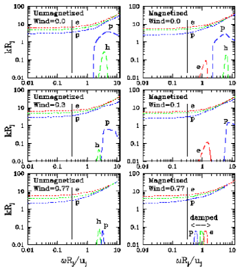
Figure 13: Pinch, helical and elliptical first body mode solutions to the dispersion relation for an unmagnetized (left column) and a magnetized (right column) external wind medium. Notation is identical to that of Figures 10, 11, & 12.

Even in the absence of a wind, the low magnetosonic Mach numbers guarantee that body mode growth rates, with the exception of the first pinch body mode, will be small. The first pinch body mode has a significant growth rate when the wind speed is low. The addition of a wind and, in particular, of a magnetized wind reduces these growth rates even further and at the highest magnetized wind speed the body modes are damped.

4 Interpretation of Simulation Results

In simulations P and T the flow velocity is sub-Alfvénic for the inlet conditions and thus enters the computational grid stable to helical and higher order modes of jet distortion, although not stable to the fundamental pinch mode. While in both simulations the jet becomes super-Alfvénic within a few jet radii of the inlet, both jets would remain stable beyond this point even in the absence of an external magnetized wind as a result of their density. For example, in simulation P the jet should remain stable to helical and higher order modes until $z\sim 10R_{0}$ when $u_{j}^{2}-(1+\eta)V_{Aj}^{2}>0$, where $\eta\equiv\rho_{j}/\rho_{e}$ and $V_{Aj}\equiv[B_{j}^{2}/(4\pi\rho_{j})]^{1/2}$. However, at this distance the wind speed has already risen sufficiently, $u_{e}\sim 0.2a_{e}$, so that $(u_{j}-u_{e})^{2}-(1+\eta)V_{Aj}^{2}<0$ and the jet is stable to helical and higher order modes even in the absence of a magnetic field in the wind. Simulation P remains stable to helical and higher order modes out to $z\sim 30R_{0}$ where finally $(u_{j}-u_{e})^{2}-V_{As}^{2}>0$, where $V_{As}\equiv[(\rho_{j}+\rho_{e})(B_{j}^{2}+B_{e}^{2})/(4\pi\rho_{j}\rho_{e})]^{1/2}$. Simulation T exhibits no such magnetized wind and destabilizes to helical and higher order modes when $u_{j}^{2}-(1+\eta)V_{Aj}^{2}>0$ at $z\sim 12R_{0}$.

In general, normal mode solutions come in pairs where the slightly faster moving wave (forwards moving in the jet fluid frame) is damped and the more slowly moving wave (backwards moving in the jet fluid frame) is growing. As the wind speed increases the spatial growth rate of helical and higher order surface modes decreases as the velocity shear decreases and the wave speed, measured in the stationary observer frame, increases. However, the fundamental pinch mode wave speed (in the jet fluid frame a backwards moving slow magnetosonic wave) and growth rate remain relatively unchanged as wind speed increases. At some intermediate wind speed, the faster moving (forwards moving in the jet fluid frame) helical and higher order surface mode wave speed becomes comparable to the speed of the fundamental pinch mode and now these waves are growing whereas the slower moving helical and higher order surface modes are damped. Here the fundamental pinch and the helical and higher order surface modes are growing with comparable growth rates. The intermediate wind speed value depends on the magnetization of the wind and occurs at much lower wind speed for a magnetized wind. As wind speeds rise above this intermediate speed all growth rates are reduced, but a larger wind speed is required to achieve reduction in the fundamental pinch mode growth rate.

The different dependence of the fundamental pinch and the higher order surface mode growth rates to the presence of an external wind explains the stabilization of simulation P to a distance well beyond the Alfvén point, and also explains the presence of emission knots in the jet in simulation P at intermediate simulation times. In particular, the emission knots, visible in Figure 9 at distances $25<z/R_{0}<35$, with $\lambda\lesssim 4R_{0}\sim 3.5R_{j}$ and with $v_{w}\sim 0.85a_{e}\sim 0.45u_{j}$ can be identified with the fundamental pinch mode. If we apply the parameters given in Table 2 for simulation P we find that the observed knot spacing corresponds theoretically to an angular frequency $\omega R_{j}/u_{j}\sim 1$. This frequency corresponds to the maximum growth rate for an unmagnetized stationary external medium (see the top left panel in Figure 10) and to the lowest frequency at which the growth rate is comparable to the maximum growth rate in the presence of a low speed magnetized external wind (see the bottom left panel in Figure 11). At these intermediate times and at this distance from the inlet the large magnetized winds seen at the end of the simulation have not yet developed. The lower magnetized wind speeds at intermediate times, $u_{e}\sim 0.15-0.35a_{e}^{ms}$, suppress the helical and higher order modes leaving the fundamental pinch mode to dominate and produce the observed emission knots. The absence of a significant wind in simulation T results in no suppression of helical and higher order surface mode instability. Thus, in simulation T these normal modes dominate the dynamics at all times and have suppressed the development of the fundamental pinch mode and accompanying emission knots.

In order to make some quantitative comparison with structures observed in the numerical simulations at large distances from the inlet we have solved the dispersion relation for parameters typical to the jet at $z/R_{0}=$ 35 & 50. The parameters used for these distances are given in Table 3 and $p_{e}/p^{*}_{e}=1$ and $a_{e}^{ms}=a_{e}$; recall that Table 2 contains jet parameters for $z/R_{0}=18$.

Table 3: Parameters at $z\sim$ 35 & 50R₀

Sim @ z/R0	$\eta$	$u_{j}/a_{e}$	$a_{j}/a_{e}$	$\omega R_{j}/u_{j}$	$M_{j}$	$M^{A}_{j}$	$M^{ms}_{j}$	$p_{j}/p^{*}_{j}$
P @ 35	0.35	2.0	0.93	0.36	2.15	1.60	1.25	0.40
P @ 50	0.45	2.0	0.85	0.41	2.35	2.00	1.50	0.46
T @ 50	0.45	2.2	1.00	0.37	2.20	1.46	1.22	0.35

In simulation P at $z/R_{0}<30$ the short wavelength, $\lambda\lesssim 5R_{0}$, low amplitude oscillation in $p^{*}$ and $v_{z}$ is consistent with the weak fundamental pinch mode instability that remains at the highest magnetized wind speeds. The jet destabilizes at about $z/R_{0}=30$ and at $30<z/R_{0}<50$ exhibits a dominant oscillation in $v_{x}$ ($v_{r}$) with $\lambda\lesssim 8R_{0}\sim 5.3R_{j}$, where $R_{j}\sim 1.5R_{0}$ at $z/R_{0}=40$. The observed wavelength is consistent with a growing elliptical distortion at frequency $\omega R_{j}/u_{j}\sim 0.4$ for the relatively low wind speeds, $u_{e}/a_{e}^{ms}\lesssim 0.2$ found at $z/R_{0}\sim 40$, and an elliptical distortion is evident in the cross sections in panels 30 and 35 in Figure 6. At $z>55R_{0}$ dominant out of phase transverse velocity oscillations indicative of helical twisting with $\lambda\sim 10R_{0}\sim 6R_{j}$ moving with $v_{w}\sim 0.75a_{e}\sim 0.40u_{j}$ are consistent with precession induced helical twisting for the observed low wind speeds of $u_{e}/a_{e}^{ms}\sim 0.2$. Thus, the initial precession frequency is preserved through the instability point. Movement of the jet center off the $z$-axis appears at $z\geq 40$ in the cross section panels in Figure 6.

In simulation T at $z<40R_{0}$ a region of growing amplitude oscillations in $p^{*}$, $v_{z}$ and $v_{x}$ with $\lambda\lesssim 8R_{0}$ can be readily identified with an elliptical distortion seen in cross sections in Figure 6 from $10\leq z/R_{0}\leq 30$. We find that the observed elliptical distortion is consistent with the elliptical surface mode solutions determined from parameters appropriate to simulation T at $z/R_{0}=18$ with $\lambda\sim 6.5R_{j}$ when $\omega R_{j}/u_{j}\sim 0.25$. At $z>40R_{0}$ dominant out of phase transverse velocity oscillations indicative of helical twisting with $\lambda\sim 10R_{0}$ moving with $v_{w}\sim 0.41u_{j}$ are readily identified with the expected precession driven helical surface mode solution as was found for simulation P. The simulations indicate and the theoretical solution to the dispersion relation confirms that the helical mode is relatively insensitive to the exact values of the Mach number or to the wind magnetization and low wind speed found in the simulations at these large distances from the inlet.

In both simulations the magnitude of the toroidal velocity induced by helical twisting declines approximately as $\exp[-2(r/R_{j}-1)]$ for $r\geq R_{j}$, and the flow field remains well organized out to $r>3R_{j}$ even though the magnitude of the toroidal velocity declines rapidly. The direction of the toroidal velocity field along the line-of-sight oscillates with a sinusoidal wavelength equal to the helical wavelength, i.e., $\sim 10R_{0}$. This toroidal velocity field orients the poloidal magnetic field in simulation P parallel and anti-parallel to the line-of-sight with the banded structure shown in Figure 8. In simulation T a similar toroidal velocity field, albeit with magnitude $\approx 2/3$ of that in simulation P, cannot reorient the poloidal field component to overcome the orientation of the initial toroidal field component.

5 Implications

We have shown that jets can be stabilized to the KH helical and higher order asymmetric normal modes provided the velocity shear, $\Delta u\equiv u_{j}-u_{e}$, between the jet and the external medium is less than a “surface” Alfvén speed, $V_{As}\equiv[(\rho_{j}+\rho_{e})(B_{j}^{2}+B_{e}^{2})/(4\pi\rho_{j}\rho_{e})]^{1/2}$. Thus, the presence of a magnetic field in the external medium and the presence of an outflowing wind in the external medium are stabilizing. At relatively high magnetized wind speeds all normal modes are effectively stabilized. At more modest wind speeds or when the jet is sub-Alfvénic the fundamental pinch mode remains unstable while the helical and higher order modes can be partially or completely stabilized. In this case the fundamental pinch mode dominates the dynamics and emission knots can be produced in an initially steady flow, albeit the simulations considered here contain an initial precessional perturbation. The initially stable poloidal magnetic field simulation shows that the small amplitude precessional perturbation is effectively communicated down the jet to the point where the jet becomes unstable. We note here that the wave speed in the stable region is not as stated in paper I. The wave speed is given properly by equation (4) in this paper with the previously stated result, $v_{w}\approx u_{j}+V_{Aj}$, only appropriate in the dense jet limit. The precessional perturbation couples to growing helical jet distortions in the super-magnetosonic regime which are identical for the poloidal and helical magnetic field simulations. The helical twist leads to a very well organized toroidal velocity field within (see Figure 2) and outside of the jet. The toroidal velocity field orients any poloidal magnetic field inside and outside the jet along the direction of the toroidal velocity. We note that mixing in simulation P has spread the poloidal field out to $r\lesssim 2R_{j}$, but the velocity field remains well ordered out to $r\sim 3R_{j}$. Thus, a poloidal magnetic field in the medium surrounding a jet could be ordered by a helically induced toroidal velocity field out to larger distance than seen in simulation P.

5.1 Protostellar Jets

Recent work has suggested that protostellar jets may operate in the low magnetosonic Mach number regime as low magnetosonic Mach numbers are expected for magnetically launched jets (Fendt & Camenzind 1996; Lery & Frank 2000). However, the low magnetosonic Mach number regime is typically KH unstable to helical and higher order normal modes. In such a situation, helical and other higher order asymmetric distortions would be expected to dominate the dynamics and appearance of these jets. This fact has been demonstrated by somewhat higher Mach number numerical simulations (Xu, Hardee, & Stone 2000). While there is evidence for helical and other asymmetric distortions in protostellar jets, many of these jets contain emission knots along a relatively straight jet, e.g., the knotty HH 34 jet which lies within a weak CO outflow (Reipurth et al. 1986; Chernin & Masson 1995; Devine et al. 1997). A more complex example is provided by the HH 111 jet (Reipurth et al. 1997) which shows emission knots in an initially relatively straight jet but with an apparent sinusoidal oscillation and staggered bow shocks at larger distance. Here the jet is surrounded by a bubble within a larger molecular outflow (Nagar et al. 1997; Cernicharo & Reipurth 1996). The HH 34 and HH 111 jets are shown in Figure 14.

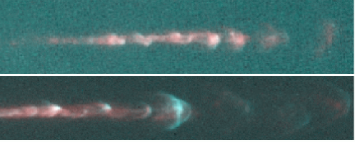
Figure 14: Images of (top) HH 34 and (bottom) HH 111 (Devine et al. 1997; Reipurth et al. 1997).

In addition to HH 34 and HH 111, observations have shown that other protostellar jets are embedded in slower and less collimated molecular outflows (see Richer et al. 2000 and references therein). These outflows typically surround but do not necessarily directly interact dynamically with the more highly collimated jet, i.e., there is no direct observational evidence for a significant wind in the material immediately outside the jet. That there might be a significant wind environment around a more highly collimated jet is suggested by studies of jet formation and collimation from an accretion disk, e.g., Meier, Koide, & Uchida (2001) and Begelman & Blandford (1999) in the extragalactic context and Königl & Pudritz (2000), Contopoulos & Sauty (2001) and Lery et al. (2002) in the protostellar context, or by $X$-wind models in the protostellar context (e.g., Shu et al. 2000). While the properties of the wind close to the jet are important, the manner in which the wind is produced and its properties far from the jet are not important. The rapid exponential decline in velocity fluctuations outside the jet implies an interaction layer of only a few jet radii in thickness, and it does not matter whether a wind is produced as part of the entrainment and mixing process (as in the present simulations) or a wind originates in some other fashion (see Lery et al. (2002) for some discussion of disk winds and $X$-winds, and the relation between protostellar jets and molecular outflows).

Our present results suggest that if the magnetosonic Mach number of a protostellar jet is sufficiently low, then a low speed magnetized wind with 10% of the jet speed (or significantly higher unmagnetized wind speed) could stabilize the jet to helical and higher order modes of asymmetric jet distortion while leaving the fundamental pinch mode to grow and provide a trigger for knot spacing not too different from what is seen in the protostellar jets. Note that the present results indicate that the wind need extend no more than a few jet radii beyond the faster highly collimated jet material. Spatial change in the wind speed such as a lower wind speed at larger distance from the source would allow helical and higher order modes to grow, triggered by precession at the origin. Thus, it is possible that the interaction between a low magnetosonic Mach number protostellar jet and an appropriate outflowing wind could trigger knot formation with spacing similar to that observed in the HH 34 and HH 111 jets without requiring quasi-episodic jet injection on short timescales.

The present numerical and theoretical results do not include the effects of radiative cooling that are important on protostellar jets or the effect of much higher jet density relative to the external medium. In general, the inclusion of radiative cooling leads to greater instability (Stone et al. 1997; Xu et al. 2000). However, previous 2D (Hardee & Stone 1997) and unpublished theoretical results indicate that the presence of significant magnetic field reduces the difference between the stability properties of radiatively cooled and adiabatic jets.

5.2 Extragalactic Jets

The poloidally magnetized jet in simulation P shows surface corrugations even before it destabilizes and after destabilization shows significant cross section distortions in addition to elliptical distortion and large scale helical twisting. In simulation T the presence of significant toroidal magnetic field component suppresses the filamentation seen on the poloidally magnetized jet. While the jet in simulation T exhibits elliptical distortion and helical twisting all higher order normal modes are suppressed. This effect was observed in paper I and in supermagnetosonic jet simulations containing a significant toroidal magnetic field component (RHCJ). No significant mass entrainment occurs in the stable region in the poloidally magnetized simulation P but significant mass entrainment accompanies the development of elliptical distortion and helical twisting where the jet destabilizes. In simulation T, there is also evidence for mass entrainment beginning where the jet destabilizes and elliptical distortion appears. Simulation P shows significantly less entrainment and slowing of ordered flow than was observed in the comparable “light” jet simulation (simulation B in paper I), and this result confirms that denser jets are more robust. Simulation T could not be run long enough to make a similar assessment, but it is clear from paper I, the results here, and results from other work (RHCJ) that a significant toroidal magnetic field helps to reduce entrainment and helps to maintain jet collimation.

The line-of-sight appearance of the low magnetosonic Mach number poloidally magnetized jets both here and in paper I when they become unstable appears plume like. Simulations at somewhat higher magnetosonic Mach numbers with primarily poloidal or weak toroidal magnetic field (Rosen, Hardee, Clarke, & Johnson 1999; Rosen & Hardee 2000) also appear plume like. This set of poloidal and weak toroidal magnetic field simulations seems most representative of the lower power FR I type extragalactic jets whose appearance has been argued (see Bicknell 1994, 1995) to be the result of significant mass entrainment. Surface turbulence from KH instability has been proposed previously as a mechanism for the production of the high observed RM (rotation measure) associated with some of the FR I radio sources (Bicknell et al. 1990), although other authors have pointed out quantitative difficulties with this mechanism (Taylor & Perley 1993; Ge & Owen 1993). Quantitative difficulties take the form of requiring an excessively large magnetic field in a thin Faraday layer or require a Faraday layer thicker than, for example, the dimension of the RM structure in order to produce the observed RM with more modest magnetic fields.

The simulation results presented in RHCJ, Rosen & Hardee (2000) and in paper I revealed large scale organization in line-of-sight emission image structure and in the accompanying B-field vectors associated with helical twisting and mass entrainment. These organized structures extended throughout the mixing region and formed a relatively thick layer around a central jet spine. This occurred if polarization B-field vectors were aligned with the jet flow or if polarization B-field vectors were transverse to the jet flow if the toroidal magnetic fields were sufficiently below equipartition. The present work reveals that the ordering is accomplished by the flow field associated with helical twisting, should extend to at least a jet diameter beyond the central jet spine, and can produce positive and negative RM bands that alternate and lie across a jet. The sum total of all the work suggests that ordering by the flow field outside the jet spine requires a primarily poloidal magnetic field in the mixing region and/or in the cocoon environment surrounding the jet/tail. Our present simulations do not specifically address the issue of poloidal field alignment in the mixing region or in the external medium in extragalactic sources but we note that the polarization vectors in the 3C 31 jets suggest a poloidal orientation of the magnetic field in a sheath even though the vectors suggest toroidal orientation of the magnetic field in the jet spine (Laing 1996).

Recently Eilek & Owen (2002) have considered the high RM structure associated with radio source 3C 465 in Abell cluster A2634 shown in Figure 15.

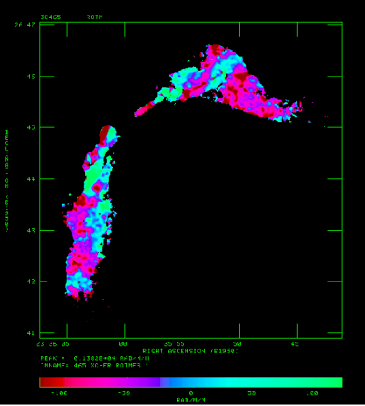
Figure 15: Rotation measure distribution in Abell 2634 (3C 465). The colors are chosen to distinguish positive (green & light blue) and negative (red & dark blue) values; $1\arcmin$ is 35.2 kpc (from Eilek & Owen 2002).

In particular the west jet/tail of this radio source, whose B-field vectors more or less follow the tail, show positive and negative RM bands that alternate and lie across the tail. The emission and RM images can be taken to suggest organization resulting from helical twisting of the jet/tail flow. The observations suggest a typical scale size for the RM bands of $\sim 1\arcsec$ or about 0.7 kpc, and Eilek & Owen find that a similarly dimensioned thin $\sim 0.7$ kpc Faraday layer requires an excessively large, $\sim 96\mu G$ and vastly overpressured, $p_{b}/p_{g}\sim 420$ magnetic field to produce the observed RM. Thus, they conclude that the more likely candidate is a thick Faraday screen associated with ordered much weaker cluster magnetic fields. However, in 3C 465 the jet/tail diameter, as inferred from the transverse extent of the radiating material, at the location of the alternating RM bands is $\lesssim 5\arcsec$ or about 3 kpc. If we associate this distance with the thickness of a Faraday screen then the magnetic field required to produce the observed RM is reduced to $\sim 20\mu G$ and $p_{b}/p_{g}\approx 25$. If the jet/tail is not in the plane of the sky, the line-of-sight through the sheath will be longer. While the required magnetic field is still high, we conclude that RM structure in some radio sources may be associated with large scale flow field organization of an ambient and/or jet magnetic field in a thick sheath around a central jet spine.

P. Hardee and A. Rosen acknowledge support from the National Science Foundation through grant AST-9802995 to the University of Alabama. The numerical work utilized the Cray T90 at the San Diego Supercomputing Center (operated under the auspices of the National Partnership for Advanced Computational Infrastructure, NPACI).

References

- (1)
- (2) Appl, S. 1996, in ASP Conf. Series Vol. 100: Energy Transport in Radio Galaxies and Quasars, eds. P.E. Hardee, A.H. Bridle & A. Zensus, (San Francisco: ASP), 129
- (3) Appl, S., & Camenzind, M. 1992, A&A, 256, 354
- (4) Appl, S., Lery, T., & Baty, H. 2000, A&A, 355, 818
- (5) Begelman, M.C. 1998, ApJ, 493, 291
- (6) Begelman, M.C., & Blandford, R.D. 1999, MNRAS, 303, L1
- (7) Bicknell, G.V. 1994, ApJ, 422, 542
- (8) Bicknell, G.V. 1995, ApJS, 101, 29
- (9) Bicknell, G.V., Cameron, R.A., & Gingold, R.A. 1990, ApJ, 357, 373
- (10) Bodo, G., Massaglia, S., Rossi, P., Rosner, R., Malagoli, A., & Ferrari, A. 1995, A&A, 303, 281
- (11) Bodo, G., Rosner, R., Ferrari, A., & Knoblock, E. 1989, ApJ, 341, 631
- (12) Camenzind, M. 1997, in IAU Symp. 182: Herbig-Haro Flows and the Birth of Low Mass Stars, eds. B. Reipurth & C. Bertout, (Dordrecht: Kluwer), 241
- (13) Cernicharo, J., & Reipurth, B. 1996, ApJ, 460, 57
- (14) Chernin, L.M., & Masson, C.R. 1995, ApJ, 443, 181
- (15) Clarke, D.A. 1996, ApJ, 457, 291
- (16) Clarke, D.A., Norman, M.L., & Burns, J.O. 1989, ApJ, 342, 700
- (17) Contopoulos, I., & Sauty, C. 2001, A&A, 365, 165
- (18) Devine, D., Bally, J., Reipurth, B., & Heathcote, S. 1997, AJ, 114, 2095
- (19) Eilek, J.A., & Owen, F.N. 2002, ApJ, 567, 202
- (20) Fendt, C., & Camenzind, M. 1996, A&A, 313, 591
- (21) Ferrari, A., Trussoni, E., & Zaninetti, L. 1981, MNRAS, 196, 1051
- (22) Fiedler, R., & Jones, T.W. 1984, ApJ, 283, 532
- (23) Ge, J.P., & Owen, F.N. 1993, AJ, 105, 778
- (24) Hardee, P.E. 1984, ApJ, 287, 523
- (25) Hardee, P.E., Clarke, D.A., & Rosen, A. 1997, ApJ, 485, 533
- (26) Hardee, P.E., & Rosen, A. 1999, ApJ, 524, 650 (paper I)
- (27) Hardee, P.E., & Stone, J.M. 1997, ApJ, 483, 121
- (28) Königl, A., & Pudritz, R.E. 2000, Protostars and Planets IV, eds. Mannings, V., Boss, A.P., Russell, S.S. (Tucson: University of Arizona Press), 759
- (29) Laing, R.A. 1996, in ASP Conf. Series Vol. 100: Energy Transport in Radio Galaxies and Quasars, eds. P.E. Hardee, A.H. Bridle & A. Zensus, (San Francisco: ASP), 241
- (30) Lery, T., Baty, H., & Appl, S., 2000, A&A, 355, 1201
- (31) Lery, T., & Frank, A. 2000, ApJ, 533, 897
- (32) Lery, T., Henriksen, R.N., Fiege, J.D., Ray, T.P., Frank, A., & Bacciotii, F. 2002, A&A, in press (astro-ph/0203090)
- (33) Meier, D.L., Payne, D.G., & Lind, K.R. 1996, in IAU Symp. 175: Extragalactic Radio Sources, eds. R. Eckers, C. Fanti & L. Padrielli, (Dordrecht: Kluwer), 433
- (34) Meier, D.L., Edgington, S., Godon, P., Payne, D.G., & Lind, K.R. 1997, Nature, 388, 350
- (35) Meier, D.L., Koide, S., & Uchida, Y. 2001, Science, 291, 84
- (36) Nagar, N.M., Vogel, S.N., Stone, J.M., & Ostriker, E.C. 1997, ApJ, 482, L195
- (37) Owen, F.N., Hardee, P.E., & Cornwell, T.J. 1989, ApJ, 340, 698
- (38) Ouyed, R., Pudritz, R.E., & Stone, J.M. 1997, Nature, 385, 409
- (39) Ouyed, R., & Pudritz, R.E. 1997, ApJ, 482, 712
- (40) Ray, T.P. 1981, MNRAS, 196, 195
- (41) Reipurth, B., Bally, J., Graham, J.A., Lane, A.P., & Zealey, W.J. 1986, A&A, 164, 51
- (42) Reipurth, B., Hartigan, P., Heathcote, S., Morse, J.A., & Bally, J. 1997, AJ, 114, 757
- (43) Richer, J.S., Shepherd, D.S., Cabrit, S., Bachiller, R., & Churchwell, E. 2000, in Protostars and Planets IV, ed. V. Mannings, A.P. Boss, & S.S. Russell (Tucson: Univ. Arizona Press), 867
- (44) Romanova, M.M., Ustyugova, G.V., Koldoba, A.V., Chechetkin, V.M. & Lovelace, R.V.E. 1997, ApJ, 482, 708
- (45) Rosen, A., & Hardee, P.E. 2000, ApJ, 542, 750
- (46) Rosen, A., Hardee, P.E., Clarke, D.A., & Johnson, A. 1999, ApJ, 510, 136 (RHCJ)
- (47) Shu, F.H., Najita, J.R., Shang, H., & Li, Z.-Y. 2000 Protostars and Planets IV, eds. Mannings, V., Boss, A.P., Russell, S.S. (Tucson: University of Arizona Press), 789
- (48) Stone, J.M., Xu, J., & Hardee, P.E. 1997, ApJ, 483, 136
- (49) Stone, J.M., Hawley, J.F., Evans, C.E., & Norman, M.L. 1992, ApJ, 388, 19
- (50) Taylor, G.B., & Perley, R.A. 1993, ApJ, 416, 554
- (51) van Leer, B. 1977, J. Comput. Phys. 23, 276
- (52) Xu, J., Hardee, P.E., & Stone, J.M. 2000, ApJ, 543, 161
- (53)