High Mass X-ray Binaries as a Star Formation Rate Indicator in Distant Galaxies

Abstract

Based on CHANDRA and ASCA observations of nearby starburst galaxies and RXTE/ASM, ASCA, and MIR-KVANT/TTM studies of high mass X-ray binary (HMXB) populations in the Milky Way and Magellanic Clouds, we propose that the number and/or the collective X-ray luminosity of HMXBs can be used to measure the star formation rate (SFR) of a galaxy. We show that, within the accuracy of the presently available data, a linear relation between HMXB number and star formation rate exists. The relation between SFR and collective luminosity of HMXBs is non-linear in the low SFR regime, $L_{X}\propto\text{SFR}^{\sim 1.7}$, and becomes linear only for sufficiently high star formation rate, SFR$\ga 4.5$ M_⊙ yr^-1 (for M${}_{*}>8$M_⊙). The non-linear $L_{X}-SFR$ dependence in the low SFR limit is not related to non-linear SFR-dependent effects in the population of HMXB sources. It is rather caused by the fact, that we measure the collective luminosity of a population of discrete sources, which might be dominated by the few brightest sources. Although more subtle SFR-dependent effects are likely to exist, in the entire range of SFRs the data are broadly consistent with the existence of a universal luminosity function of HMXBs which can be roughly described as a power law with a differential slope of $\sim 1.6$, a cutoff at $L_{X}\sim{\rm few}\times 10^{40}$ erg s^-1 and a normalisation proportional to the star formation rate.

We apply our results to (spatially unresolved) starburst galaxies observed by CHANDRA at redshifts up to $z\sim 1.2$ in the Hubble Deep Field North and show that the calibration of the collective luminosity of HMXBs as a SFR indicator based on the local sample agrees well with the SFR estimates obtained for these distant galaxies with conventional methods.

1 Introduction

X-ray observations open a new way to determine the star formation rate (SFR) in young very distant galaxies. CHANDRA observations of actively star forming galaxies in our vicinity, RXTE/ASM, ASCA, and MIR-KVANT/TTM data about high-mass X-ray binary (HMXB) populations in our Galaxy and the Magellanic Clouds provide a possibility to calibrate the dependence of SFR on the X-ray luminosity of a galaxy due to HMXBs. For nearby, spatially resolved galaxies for which CHANDRA is able to resolve individual X-ray binaries we also have the opportunity to calibrate the dependence of SFR on the total number of HMXB sources.

In the absence of a bright AGN, the X-ray emission of a galaxy is known to be dominated by the collective emission of its X-ray binary populations (see e.g. Fabbiano (1994)). X-ray binaries, conventionally divided into low and high mass X-ray binaries, consist of a neutron star (NS) or a black hole (BH) accreting from a normal companion star. To form a NS or BH the initial mass of the progenitor star must exceed $\sim$ 8 M_⊙ (Verbunt & van den Heuvel, 1994). The main distinction between LMXBs and HMXBs is the mass of the optical companion with a broad, thinly populated dividing region between $\sim 1-5$ M_⊙. This difference results in drastically different evolution time-scales for low and high mass X-ray binaries and, hence, different relations of their number and collective luminosity to the instantaneous star formation activity and the stellar content of the parent galaxy. In the case of a HMXB, having a high mass companion, generally $M_{optical}\ga 10$ M_⊙ (Verbunt & van den Heuvel, 1994), the characteristic time-scale is at most the nuclear time-scale of the optical companion which does not exceed $\sim 2\cdot 10^{7}$ years whereas for a LMXB, generally $M_{optical}\la 1$ M_⊙, it is of the order of $\sim 10^{10}$ years.

HMXBs were first recognised as short-living objects fed by the gas supply of a massive star as a result of the discovery of Cen X-3 as an X-ray pulsar by UHURU, in a binary system with an optical companion of more than 17 M_⊙ (Schreier et al., 1972), and the localisation and mass estimation of the Cyg X-1 BH due to a soft/hard state transition occurring simultaneously with a radio flare (Tananbaum et al., 1972), and following optical observations of a bright massive counterpart (Bolton, 1972; Lyutyi et al., 1973). Dynamics of interacting galaxies, e.g. Antennae, provide an additional upper limit on the evolution and existence time-scale of HMXBs since the tidal tails and wave patterns in which star formation is most vigorous are very short-lived phenomena, of the order of a crossing time of interacting galaxies (Toomre & Toomre, 1972; Eneev et al., 1973).

The prompt evolution of HMXBs makes them a potentially good tracer of the very recent star formation activity in a galaxy (Sunyaev et al., 1978) whereas, due to slow evolution, LMXBs display no direct connection to the present value of SFR. LMXBs rather are connected to the total stellar content of a galaxy determined by the sequence of star formation episodes experienced by a galaxy during its lifetime (Ghosh & White, 2001; Ptak et al., 2001; Grimm et al., 2002).

Several calibration methods are employed to obtain SFRs using UV, FIR and radio flux from distant galaxies. Many of these methods rely on a number of assumptions about the environment in the galaxy and suffer from various uncertainties, e.g. the influence of dust, escape fraction of photons or the shape of the initial mass function (IMF). An additional and independent calibrator might therefore become a useful method for the determination of SFR. Such a method, based on the X-ray emission of a galaxy, might circumvent one of the main sources of uncertainty of conventional SFR indicators – absorption by dust and gas. Indeed, galaxies are mostly transparent to X-rays above about 2 keV, except for the densest parts of the most massive molecular clouds.

The existence of various correlations between X-ray and optical/far-infrared properties of galaxies has been noted and studied in the past. Based on Einstein observations of normal and starburst galaxies from the IRAS Bright Galaxy Sample, Griffiths & Padovani (1990) and David et al. (1992) found correlations between the soft X-ray luminosity of a galaxy and its far-infrared and blue luminosity. Due to the limited energy range (0.5–3 keV) of the Einstein observatory data one of the main obstacles in quantifying and interpreting these correlations was proper accounting for absorption effects and intrinsic spectra of the galaxies which resulted in considerable spread in the derived power law indices of the X-ray – FIR correlations, $\sim 0.7-1.0$. Moreover, supernova remnants are bright in the soft band of the Einstein observatory. CHANDRA, however, is able to distinguish SNRs from other sources due to its sensitivity to harder X-rays. Although the X-ray data were not sufficient to discriminate between contributions of different classes of X-ray sources, David et al. (1992) suggested that the existence of such correlations could be understood with a two component model for X-ray and far-infrared emission from spiral galaxies, consisting of old and young populations of the objects having different relations to the current star formation activity in a galaxy. The uncertainty related to absorption effects was recently eliminated by Ranalli et al. (2002), who extended these studies to the harder energy band of 2–10 keV based on BeppoSAX and ASCA data. In particular, they found a linear correlation between total X-ray luminosity of a galaxy and both radio and far-infrared luminosities and suggested that the X-ray emission might be directly related to the current star formation rate in a galaxy and that such a relation might also hold at higher redshifts.

Table 1: The primary sample of local galaxies used to study the luminosity function of HMXB sources.

Source	Hubble	distance(b)	SFR(c)	Mdynamical	Ref.(d)	SFR/M	$N(L>$	$L_{X,total}$	Ref.(e)
	type(a)	[Mpc]	[M⊙ yr-1]	[$10^{10}$M⊙]		[$10^{-10}$yr-1]	$2\cdot 10^{38}$erg s-1)	[$10^{39}$ erg s-1]
N3256	Sb(s) pec	35.0	44.0	5.0	(i)	8.8	12	128	(1)
Antennae	Sc pec	19.3	7.1	8.0	(i)	0.9	27	49	(2)
M 100	Sc(s)	20.4	4.8	24.0	(ii)	0.2	5	10	(3)
M 51	Sbc(s)	7.5	3.9	15.0	(iii)	0.26	15	16	(4)
M 82	Amorph	5.7	3.6	1.0	(iv)	3.6	12	23	(5)
M 83	SBc(s)	3.8	2.6	15.4	(v)	0.17	2	0.14	(6)
N4579(f)	Sab(s)	23.5	2.5	-	-	-	5	26	(7)
M 74	Sc(s)	12.0	2.2	14.3	(vi)	0.15	8	14	(8)
Circinus(g)	Sb	3.7	1.5	2.2	(v)	0.73	6	5	(9)
N4736	RSab(s)	4.5	1.1	7.0	(v)	0.16	4	4	(6)
N4490	Scd pec	8.6	1.0	2.3	(vii)	0.43	2	1.2	(10)
N1569	Sm	2.1	0.17	0.03	(viii)	5.6	0	0.2	(11)
SMC	Im	0.06	0.15	0.2	(ix)	0.75	1	0.4	(12)
Milky Way	SAB(rs)bc	-	0.25	54	(x)	0.005	0	0.2	(13)

Table 2: The secondary sample of local galaxies used to complement the primary sample in the analysis of the $L_{X}$-SFR relation.

Source	Hubble	distance(b)	SFR(c)	Mdynamical	Ref.(d)	SFR/M	$L_{X,total}$	Ref.(e)
	type(a)	[Mpc]	[M⊙ yr-1]	[$10^{10}$M⊙]		[$10^{-10}$yr-1]	[$10^{39}$ erg s-1]
N3690	Spec	44.3	40.0	-	-	-	220	(1)
N7252	merger	68.3	7.7	4.0	(i)	1.9	94.6	(2)
N253	Sc(s)	4.2	4.0	7.3	(ii)	0.55	5.1	(3)
N4945	Sc	3.9	3.1	9.3	(ii)	0.41	8.9	(4)
N3310	Sbc(r)pec	15.3	2.2	2.0	(iii)	1.1	49.0	(1)
N891	Sb	11.1	2.1	24.0	(iv)	0.09	31.0	(1)
N3628	Sbc	10.3	1.6	16.0	(v)	0.1	13.9	(5)
IC342(g)	Scd	3.5	0.48	11.8	(ii)	0.04	0.9	(1)
LMC(h)		0.05	0.25	0.5	(vi)	0.5	0.34	(6)

The main surprise of the study presented here is that in the low SFR regime the relation between SFR and collective luminosity of HMXBs is non-linear, $L_{X}\propto{\rm SFR}^{\sim 1.7}$, and becomes linear only for sufficiently high star formation rates, when the total number of HMXB sources becomes sufficiently large. The non-linear $L_{X}-SFR$ dependence is caused by the fact that we measure the collective luminosity, that strongly depends on the brightest sources, of a population of discrete sources. We give a qualitative and approximate analytic treatment of this (purely statistical) effect below and will discuss it in more detail in a separate paper (Gilfanov et al., 2002).

There are, however, two main obstacles to use the X-ray luminosity of a galaxy as a SFR indicator. Firstly, if an active nucleus (AGN) is present in a galaxy it can easily outshine HMXBs in X-rays. In principle, the presence of an AGN component might be identified and, in some cases separated, due to different X-ray spectra of an AGN and X-ray binaries, provided a sufficiently broad band energy coverage. Secondly, there is the dichotomy into LMXBs and HMXBs which both have somewhat similar spectra that also could probably be distinguished provided sufficiently broad band coverage and sufficient signal-to-noise ratio. To estimate the SFR one is interested only in the luminosity of HMXBs, therefore the LMXB contribution needs to be subtracted. This could, in principle, be done based on an estimate of the stellar mass of a galaxy. The results of a study of the X-ray binary population of our Milky Way (Grimm et al., 2002) and knowledge of the Galactic SFR allow to estimate at which point the emission of HMXBs dominates the emission of a galaxy. This obviously depends on the ratio of SFR to stellar mass of a galaxy. We found, that roughly at a ratio of $\sim 0.05$ M_⊙ yr^-1 per $10^{10}$ M_⊙ of total dynamical mass, or $\sim 0.5$ M_⊙ yr^-1 per $10^{10}$ M_⊙ of stellar mass, the emission of HMXB sources begins to dominate the X-ray emission of a galaxy (where SFR value refers to a formation rate of stars more massive than $\sim 5$ M_⊙). It should be emphasised, however, that even in the worst case the X-ray luminosity based SFR estimate should be able to provide an upper limit on the ongoing star formation activity in a galaxy.

Future observations with present, CHANDRA and XMM, and upcoming X-ray missions, Astro-E and especially Constellation-X and XEUS, the last having 1 arc sec angular resolution and a 100 times larger effective area than CHANDRA, will permit to get information about the SFR of galaxies from X-rays even at high redshifts. We know from optical and radio data that the SFR was much higher in galaxies at z $\sim$ 2–5 (Madau & Pozzetti, 2000). Therefore we could expect that in these galaxies the contribution of HMXBs was strongly exceeding the contribution of LMXBs.

2 Sample of galaxies

The list of galaxies used in the following analysis is given in Table 1 and Table 2 along with their Hubble type, distances and other relevant parameters.

As our primary sample of local galaxies, used to study the HMXB luminosity function and to calibrate the $L_{X}$–SFR relation, we chose a number of nearby late-type/starburst galaxies observed by CHANDRA. We based our selection primarily on two criteria. Firstly, we selected galaxies that can be spatially resolved by CHANDRA sufficiently well so that the contribution of a central AGN can be discriminated and the luminosity functions of the compact sources can be constructed without severe confusion effects. We should note, however, that for the most distant galaxies from our primary sample (e.g. NGC 3256), the probability of source confusion might become non-negligible. Secondly, we limited our sample to galaxies known to have high star formation rates, so that the population of X-ray binaries is dominated by HMXBs and the contribution of low mass X-ray binaries can be safely ignored (see subsection 2.5 for more detailed discussion).

In order to probe the HMXB luminosity function in the low SFR regime, we used the results of the X-ray binary population study in the Milky Way by Grimm et al. (2002), based on RXTE/ASM observations and the luminosity function of high mass X-ray binaries in the Small Magellanic Cloud obtained by ASCA (Yokogawa et al., 2000).

The galaxies from our primary sample are listed in Table 1.

In addition, in order to increase the local sample, we selected galaxies observed by other X-ray missions, mainly ASCA, for which no luminosity function is available, but a total flux measurement. The selection was based on the requirement that no AGN-related activity had been detected and the SFR to total mass ratio is sufficiently high to neglect the LMXB contribution. These galaxies were used to complement the primary sample in the analysis of the $L_{X}$–SFR relation. They are listed in Table 2.

Finally, in order to study the $L_{X}$–SFR relation in distant galaxies at redshifts of $z\sim 0.2-1.3$ we used a number of galaxies detected by CHANDRA in the Hubble Deep Field North, see Table 4. The selection criteria are similar to those applied to the local sample and are described in more detail in Sec. 3.6.

Figure 1: Left: The luminosity functions of compact X-ray sources in nearby galaxies from the primary sample obtained by CHANDRA and listed in Table 1. The luminosity functions are plotted assuming the distances from Table 1. Right: The luminosity functions for the same galaxies scaled by the ratio of their star formation rate to the SFR of Antennae. The luminosity functions in the right panel are plotted only above their corresponding completeness limits. It is clear that despite large differences in the SFRs (by a factor of $\sim 40-50$) the scaled luminosity functions occupy only a narrow band in the $N(>L)-L$ plane.

2.1 Distances

To estimate X-ray luminosity and star formation rate, which is also based on flux measurements in different spectral bands, and compare these values for different galaxies it is necessary to have a consistent set of distances. For the galaxies from our sample, given in Tables 1 and 2 cosmological effects are not important. The distances were calculated using velocities from Sandage & Tammann (1980) corrected to the centre of mass of the Local Group and assuming a Hubble constant value of $H_{0}=70$ km s^-1 Mpc^-1. The distances are listed in Table 1 and Table 2. Note that these distances might differ from the values used in the original publications on the X-ray luminosity functions and SFRs.

Table 3: The star formation rates for the galaxies from the local sample, measured by different SFR indicators.

Source	Fluxes					SFRs
	UV1	H$\alpha$2	FIR3	radio4	Reference	UV	H$\alpha$	FIR	radio	adopted SFR
N3256		0.33	4.68		(a)		5.3	31.0
			7.1		(b)			47.0
			8.2		(c)			54.0		44
N4038/9		1.62			(d)		7.9
(Antennae)	3.22	1.36	4.50	10.90	(e)	9.2	6.7	9.0	9.1
			2.30		(f)			4.6		7.1
M 100		0.81			(d)		4.5
	3.07	0.72	3.36		(e)	9.8	3.9	7.5
			1.48		(f)			3.3		4.8
M 51	15.4	3.45	14.7	8.62	(e)	6.6	2.6	4.5	1.1
		4.68			(d)		3.5
		2.81			(g)		2.1			3.9
M 82		6.17	52.0		(h)		2.6	9.1
		9.12			(d)		3.9
	1.46	9.98	112.0	76.70	(e)	0.4	4.3	19.6	5.6
			53.0		(f)			9.2		3.6
M 83		13.50			(i)		2.6
		0.45			(j)		0.1
	32.4	12.20	34.2		(e)	3.6	2.3	2.7		2.6
N4579		0.36			(i)		2.6
		0.32			(d)		2.4
			0.43		(f)			1.3		2.5
M 74		1.23			(d)		2.3
	6.85	1.25	2.92		(e)	7.6	2.4	2.3
		1.51			(g)		2.9
			1.59		(f)			1.2		2.2
Circinus			22.3		(c)			1.6
		9.5	16.5		(k)		1.7	1.2		1.5
N4736		5.37			(d)		1.6
		5.37			(i)		1.6
	6.49	2.10	6.78	5.80	(e)	1.1	0.6	0.8	0.3	1.1
N4490		1.10	4.42		(l)		1.1	1.8
			2.31		(m)			0.9
				85a	(n)				1.0	1.0
N253	16.1	6.06	100.0	75.4	(e)	2.2	1.4	9.5	3.0
		6.46			(d)		1.5
		6.38			(o)		1.5
			68.7		(c)			6.5
			70.1		(f)			6.7		4.0
N1569		2.29			(d)		0.15
		3.14			(o)		0.2
		2.95			(p)		0.19
			4.59		(q)			0.12		0.17
N3628		0.32			(p)		0.4
			3.36		(f)			1.9
			3.12		(r)			1.8
			4.17		(k)			2.4		1.6
N4945		4.43	55.8		(k)		0.8	4.6
			46.2		(c)			3.8
			37.0		(r)			3.0		3.1
N7252			0.30		(s)			7.6
			0.31		(t)			7.8		7.7

2.2 X-ray luminosity functions

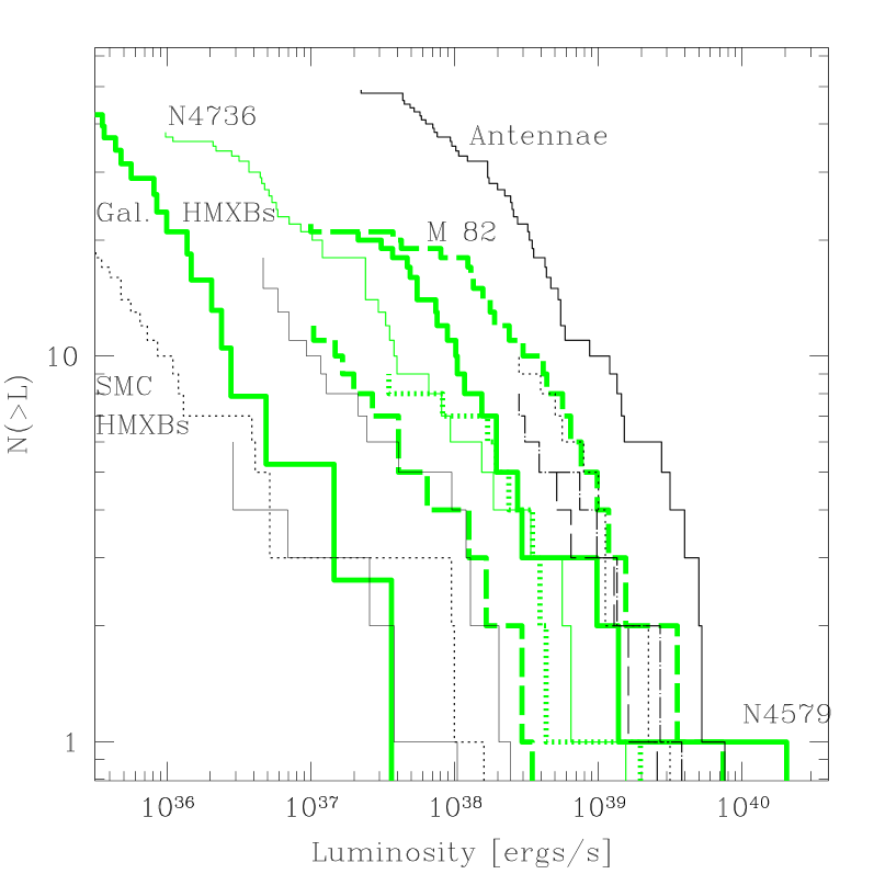
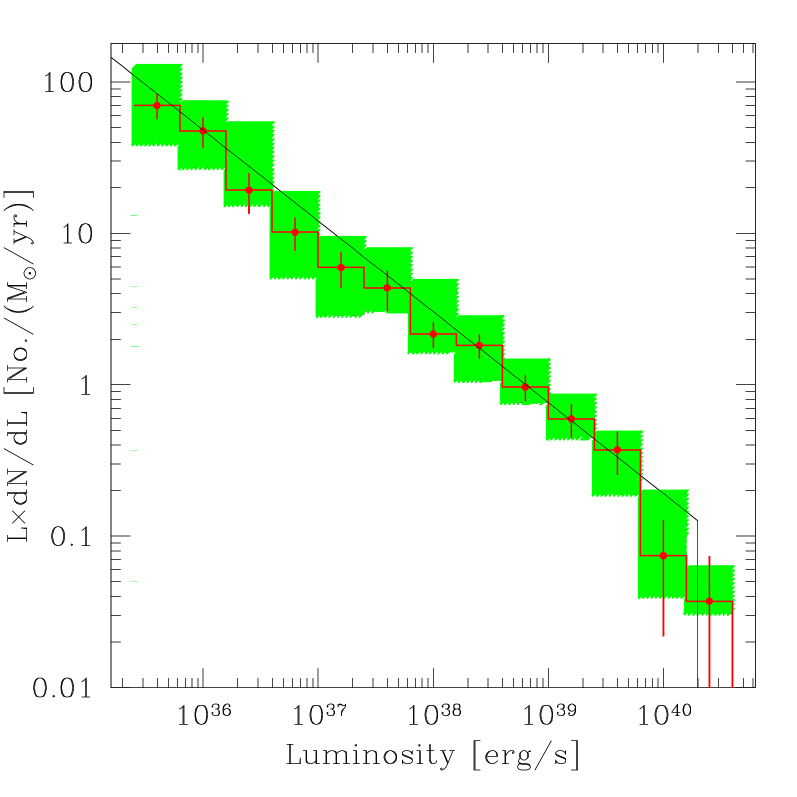
For the X-ray luminosity functions we used published results of Chandra observations of late-type/starburst galaxies. References to the original publications are given in Table 1 and Table 2. The luminosities were rescaled to the distances described in the previous subsection. Note that, due to this correction, the total X-ray luminosities and luminosities of the brightest sources might differ from the numbers given in the original publications. The complete set of luminosity functions for all objects from the primary sample (Table 1) is plotted in Fig. 1 (left panel).

One of the most serious issues important for the following analysis is the completeness level of the luminosity functions which is obviously different for different galaxies, due to different exposure times and distances. In those cases when the completeness luminosity was not given in the original publication, we used a conservative estimate based on the luminosity at which the luminosity function starts to flatten.

Due to the relatively small field of view of Chandra and sufficiently high concentration of X-ray binaries in the central parts of the galaxies the contribution of foreground and background objects can be neglected for the purpose of our analysis (e.g. M 51 (Terashima & Wilson, 2002), M 83 (Soria & Wu, 2002)). Two of the galaxies in our sample – Circinus and NGC 3256 – are located at a Galactic latitude of $|b_{II}|<20\degr$. In these cases the contribution of foreground optical stars in the Galaxy that are bright in X-rays can be discriminated based on the softness of their spectra. Extrapolating the luminosity function of X-ray binaries in the Milky Way (Grimm et al., 2002) the probability can be estimated of occurence of a foreground source due to an unknown Galactic X-ray binary with a flux exceeding the sensitivity limit of the corresponding Chandra observations. For the Chandra field of view this probability is less than $\sim 10^{-3}$ and therefore can be neglected.

The luminosities of the compact sources were derived in the original publications in slightly different energy bands, under different assumptions about spectral shape, and with different absorption column densities. Although all these assumptions affect the luminosity estimates, the resulting uncertainty is significantly smaller than those due to distance uncertainty and uncertainties in the star formation rate estimates. Moreover, in many cases, due to insufficient statistics of the data an attempt to do corrections for these effects could result in additional uncertainties, larger than those due to a small difference in e.g. energy bands. Therefore we make no attempt to correct for these differences. It should be mentioned however, that the most serious effect, up to a factor of a few in luminosity might be connected with intrinsic absorption for the sources embedded in dense starforming regions (Zezas et al., 2002). Appropriately accounting for this requires information about these sources, which is presently not available.

All the luminosity functions with exception of the Milky Way are “snapshots” of the duration of several tens of kiloseconds. On the other hand, similar to the Milky Way, compact sources in other galaxies are known to be variable. E.g. NGC 3628 is dominated by a single source, that is known to vary by about a factor of 30 (Strickland et al., 2001). This may affect the shape of the individual luminosity functions. It should not however affect our conclusions, since in the high SFR regime they are based on the average properties of sufficiently many galaxies. As for the low SFR regime, the Milky Way data are an average of the RXTE/ASM observations over four years therefore the contribution of “standard” Galactic transient sources is averaged out.

2.3 Star formation rate estimates

One of the main uncertainties involved is related to the SFR estimates. The conventional SFR indicators rely on a number of assumptions regarding the environment in a galaxy, such as dust content of the galaxy, or the shape of the initial mass function (IMF). Although comparative analysis of different star formation indicators is far beyond the scope of this paper, in order to roughly assess the amplitude of the uncertainties in the SFR estimates we compared results of different star formation indicators for each galaxy from our sample with special attention given to the galaxies from the primary sample. For all galaxies from the primary sample we found at least 3 different measurements of star formation indicators in the literature, namely UV, H$\alpha$, FIR or thermal radio emission flux. The data along with the corresponding references are listed in Table 3.

In order to convert the flux measurements to star formation rates we use the result of an empirical crosscalibration of star formation rate indicators by Rosa-Gonzalez et al. (2002). The calibration is based on the canonical formulae by Kennicutt (1998) and takes into account dust/extinction effects. We used the following flux–SFR relations:

$$SFR_{H\alpha}=1.1\cdot 10^{-41}\cdot L_{H\alpha}\text{[erg s${}^{-1}$]}$$ (1)

$$SFR_{UV}=6.4\cdot 10^{-28}\cdot L_{UV}\text{[erg s${}^{-1}$ Hz${}^{-1}$]}$$ (2)

$$SFR_{FIR}=4.5\cdot 10^{-44}\cdot L_{FIR}\text{[erg s${}^{-1}$]}$$ (3)

$$SFR_{radio}=1.82\cdot 10^{-28}\cdot\nu_{\text{G}Hz}^{0.1}\cdot L_{\nu}\text{[erg s${}^{-1}$ Hz${}^{-1}$]}$$ (4)

The last relation is from Condon (1992) and applies only to the thermal radio emission, originating, presumably, in hot gas in HII regions associated with star formation (as we used thermal 1.4 GHz flux estimates from Bell & Kennicutt (2001)).

The above relations refer to the SFR for stars more massive than $\sim 5$ M_⊙. The total star formation rate, including low mass stars, could theoretically be obtained by extrapolating these numbers assuming an initial mass function. Obviously, such a correction would rely on the assumption that the IMF does not depend on the initial conditions in a galaxy and would involve a significant additional uncertainty. On the other hand, this correction is not needed for our study as the binary X-ray sources harbour a compact object – a NS or a BH – which according to the modern picture of stellar evolution can evolve only from stars with initial masses exceeding $\sim 8$ M_⊙. The SFR correction from $M>5$ M_⊙ to $M>8$ M_⊙ is relatively small ($\sim$ 20 per cent) and, most importantly, due to the similarity of the IMFs for large masses it is significantly less subject to the uncertainty due to poor knowledge of the slope of the IMF. Thus, for the purpose of our study it is entirely sufficient to use the relations (1)–(4) without an additional correction. In the following, the term SFR refers to the star formation rate of stars more massive than $\sim 5$ M_⊙.

Since the relations (1)–(4) are based on the average properties of star forming galaxies there is considerable scatter in the SFR estimates of a galaxy obtained using different indicators (Table 3). On the other hand, the SFR estimates based on different measurements of the same indicator are generally in a good agreement with each other. A detailed study, which SFR indicator is most appropriate for a given galaxy is beyond the scope of this paper. Therefore, we relied on the fact that for all galaxies from our primary sample there are more than 3 measurements for different indicators. For each galaxy we disregarded the estimates significantly deviating from the majority of other indicators, and averaged the latter. The final values of the star formation rates we used in the following analysis are summarised in the last column of Table 3.

Figure 2: Contributions of LMXBs and HMXBs to the observed luminosity function for NGC 4736 (thin solid histogram), having smallest SFR to total mass ratio in the primary sample. The upper thick grey histogram corresponds to the contribution of HMXBs scaled from the Milky Way HMXB luminosity function by the ratio of the SFRs. The lower dotted histogram is the Galactic LMXB luminosity function scaled by the ratio of the total masses. Total masses and SFRs are given in Table 1.

2.4 Contribution of a central AGN

As mentioned in Sec. 1 the emission of a central AGN can easily outshine the contribution of X-ray binaries. However, due to the excellent angular resolution of CHANDRA it is possible to exclude any contribution from the central AGN in nearby galaxies. In our primary sample a central AGN is present in the Circinus galaxy and NGC 4579 for which the point source associated with the nucleus of the galaxy was excluded from the luminosity function. Also NGC 4945 is a case where there is contribution to the X-ray emission from an AGN. However the AGN is heavily obscured and the emission below about 10 keV of the AGN negligible (Schurch et al., 2002).

2.5 Contribution of LMXBs

Due to the absence of optical identifications of a donor star in the X-ray binaries detected by CHANDRA in other galaxies, except for LMC and SMC, there is no obvious way to discriminate the contribution of low mass X-ray binaries. On the other hand the relative contribution of LMXB sources can be estimated and, as it was mentioned above, it was one of the requirements to minimise the LMXB contribution, that determined our selection of the late-type/starburst galaxies.

Due to the long evolution time-scale of LMXBs we expect the population of LMXB sources to be roughly proportional to the stellar mass of a galaxy, whereas the population of short-living HMXBs should be defined by the very recent value of the star formation rate. Therefore the relative importance of LMXB sources should be roughly characterised by (inversely proportional to) the ratio of star formation rate to stellar mass of a galaxy. Since the determination of stellar mass, especially for a starburst galaxy, is very difficult and uncertain we used values for the total mass of a galaxy estimated from dynamical methods and assumed that the stellar mass is roughly proportional to the total mass. To check our assumption we compare the dynamical mass with the $K$ band luminosity for galaxies for which, first, enough data exist to construct a growth curve in the $K$ band and, second, for which an extrapolation to the total K band flux can be made following the approach of Spinoglio et al. (1995). The number of galaxies is small, the sample consists of M 74, M 83, NGC 4736 and NGC 891, and the uncertainties associated with this approach are big, i.e. of order a factor 3. But within this uncertainty there is a correlation between the $K$ band luminosity and the dynamical mass estimate. However, due to the more abundant data for and higher accuracy of dynamical masses we do not use stellar mass estimates based on $K$ band luminosities in the following. The values of the total dynamical mass, corresponding references, and the ratios of SFR to total mass are given in Table 1 and Table 2.

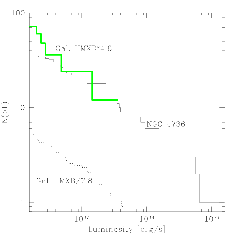
The SFR to total mass ratios for late-type galaxies should be compared with that for the Milky Way, for which the population of sufficiently luminous X-ray binaries is studied rather well (Grimm et al., 2002). We know that the Milky Way, having a ratio SFR/M_dyn $\sim 5\cdot 10^{-13}$ yr^-1, or SFR/M_stellar $\sim 5\cdot 10^{-12}$ yr^-1, is dominated by LMXB sources, HMXB sources contributing $\sim$ 10 per cent to the total X-ray luminosity and $\sim$ 15 per cent to the total number (above $\sim 10^{37}$ erg s^-1) of X-ray binaries. As can be seen from Table 1, concerning the galaxies for which luminosity functions are available the minimal value of SFR/M_dyn $\sim 1.5\cdot 10^{-11}$ yr^-1 is achieved for M 74 and NGC 4736, which exceeds by a factor of $\sim 30$ that of the Milky Way. Therefore, even in the least favourable case of these two galaxies, we expect the HMXB sources to exceed LMXBs by a factor of $\sim 3$ at least, both in number and in luminosity. A more detailed comparison is shown in Fig. 2, where we plot the expected contributions of LMXBs and HMXBs to the observed luminosity function for NGC 4736. The luminosity function of HMXBs was obtained by scaling the Milky Way HMXB luminosity function by the ratio of SFRs of NGC 4736 to the Milky Way. The LMXB contribution was similarly estimated by scaling the Milky Way LMXB luminosity function by the ratio of the corresponding total masses. As can be seen from Fig. 2, the contribution of LMXB sources does not exceed $\sim$ 30 per cent at the lower luminosity end of the luminosity function. If the fractions of NSs and BHs in low mass systems in late-type/starburst galaxies are similar to that in the Milky Way, the contribution of LMXBs should be negligible at luminosities above $\sim 10^{38}$ erg s^-1, corresponding to the Eddington limit of a neutron star, to which range most of the following analysis will be restricted.

For all galaxies from Tables 1 and 2 the lowest values for SFR/M are $4\cdot 10^{-12}$ and $9\cdot 10^{-12}$ for IC 342 and NGC 891, respectively. This means that the contribution of LMXBs could make up a sizeable portion of their X-ray luminosity, $\sim$50 per cent for IC 342 and $\sim$25 per cent for NGC 891. Therefore their data points should be considered as upper limits on the integrated luminosity of HMXBs (shown in Fig. 7 as arrows).

Figure 3: Number of sources with a 2–10 keV luminosity exceeding $2\cdot 10^{38}$ erg s^-1 versus SFR for galaxies from Table 1. The figure shows a clear correlation between the number of sources and the SFR. The straight line is the best fit from a Maximum-Likelihood fit, Eq. 5. The vertical error bars were calculated assuming a Poissonian distribution, the SFR uncertainty was assumed to be 30 per cent. For M 74 and M 100, whose completeness limit exceeds $2\cdot 10^{38}$ erg s^-1 the contribution of sources above $2\cdot 10^{38}$ erg s^-1 and below the completeness limit was estimated from the “universal” luminosity function, Eq. 7.

3 High Mass X-ray Binaries as a star formation indicator

As already mentioned, the simplest assumption about the connection of HMXBs and SFR would be that the number of X-ray sources with a high mass companion is directly proportional to the star formation rate in a galaxy. In Fig. 1 (right panel) we show the luminosity functions of the galaxies from our primary sample scaled to the star formation rate of the Antennae galaxies. Each luminosity function is plotted above its corresponding completeness limit. It is obvious that after rescaling the luminosity functions occupy a rather narrow band in the log(N)-log(L) plane and seem to be consistent with each other within a factor of $\sim 2$ whereas the star formation rates differ by a factor of $\sim 40-50$. This similarity indicates that the number/luminosity function of HMXB sources might indeed be proportional to the star formation rate. This conclusion is further supported by Fig. 3 which shows the number of sources with a luminosity above $2\cdot 10^{38}$ erg s^-1 versus the SFR. The threshold luminosity was chosen at $2\cdot 10^{38}$ erg s^-1 to have a sufficient number of galaxies with a completeness limit equal or lower than that value and, on the other hand, to have a sufficient number of sources for each individual galaxy. In addition, as was discussed in Sec. 2.5, this choice of the threshold luminosity might help to minimise the contribution of LMXB sources. The errors for the number of sources were computed assuming a Poissonian distribution. For the SFR values we assumed a 30 per cent uncertainty. Although the errors are rather big, the correlation of the number of sources with SFR is obvious. The slope of the correlation, determined from a least-squares fit in the form $N\propto SFR^{\alpha}$, is $\alpha=1.06\pm 0.07$, i.e. it is consistent with unity. A fit of this correlation with a straight line $N\propto SFR$ (shown in the figure by solid line) gives:

$$N(L>2\cdot 10^{38}\text{erg s${}^{-1}$})=(2.9\pm 0.23)\cdot SFR\text{[M${}_{\odot}$ yr${}^{-1}$]}$$ (5)

According to this fit we should expect less than 1 source in the Milky Way, having a SFR of 0.25 M_⊙ yr^-1, which is in agreement with the fact that no source above this luminosity is observed (Grimm et al., 2002).

3.1 Universal HMXB Luminosity Function ?

Figure 4: Comparison of the combined luminosity function of M 82, NGC 4579, NGC 4736 and Circinus, having SFRs in the range 1–3.5 M_⊙ yr^-1 with the Antennae luminosity function (7.1 M_⊙ yr^-1). A Kolmogorov-Smirnov test gives a probability of 15 per cent that the two luminosity functions are derived from the same distribution. See discussion in the text regarding the effect of the errors in the distance measurements on the shape of the combined luminosity function.

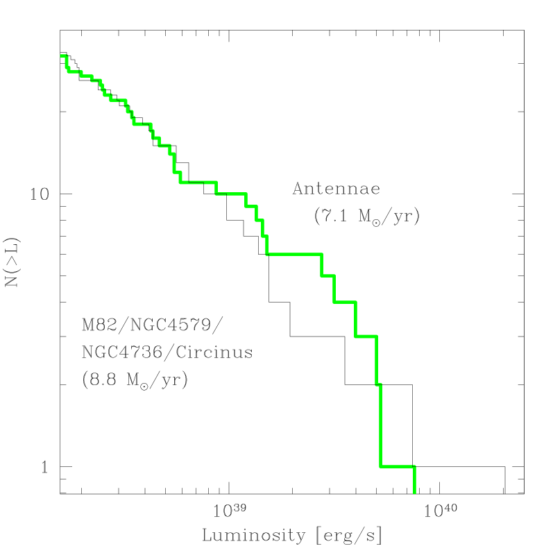
In order to check the assumption that all the individual luminosity functions have identical or similar shape with the normalisation being proportional to the SFR, we compare the luminosity function of the Antennae galaxies, having a high star formation rate ($\sim$ 7 M_⊙ yr^-1), with the collective luminosity function of galaxies with medium SFRs (in the range of $\sim$ 1.0-3.5 M_⊙ yr^-1). For the later we summed the luminosity functions of M 82, NGC 4579, NGC 4736 and Circinus, having a combined SFR of $\sim$ 8.8 M_⊙ yr^-1. The two luminosity functions (shown in Fig. 4) agree very well at $L_{X}\la 10^{39}$ erg s^-1 with possible differences at higher luminosities. In a strict statistical sense, a Kolmogorov-Smirnov test gives a 15 per cent probability that the luminosity functions are derived from the same distribution, thus, neither confirming convincingly, nor rejecting the null hypothesis. However, it should be emphasised, that whereas the shape of a single slope power law luminosity function is not affected at all by the uncertainty in the distance, more complicated forms of a luminosity function, e.g. a power law with cut-off, would be sensitive to errors in the distance determination. The effect might be even stronger for the combined luminosity functions of several galaxies, located at different distances and each having different errors in the distance estimate. In the case of a power law with high luminosity cut-off, the effect would be strongest at the high luminosity end and will effectively dilute the cut-off, as probably is observed. Therefore, we can presently not draw a definitive conclusion about the existence of a universal luminosity function of HMXBs, from which all luminosity functions of the individual galaxies are strictly derived. For instance, subtle effects similar to the effect of flattening of the luminosity function with increase of SFR suggested by Kilgard et al. (2001); Ghosh & White (2001); Ptak et al. (2001) can not be excluded based on the presently available sample of galaxies and sensitivities achieved. We can conclude, however, that there is no evidence for strong non-linear dependences of the luminosity function on the SFR.

Figure 5: Left: Combined luminosity function of compact X-ray sources in the starburst galaxies M82, NGC 4038/9, NGC 4579, NGC 4736 and Circinus with a total SFR of 16 M_⊙ yr^-1 (histogram above $2\cdot 10^{38}$ erg s^-1) and the luminosity functions of NGC 1569 and HMXBs in the Milky Way and Small Magellanic Clouds (three histograms below $2\cdot 10^{38}$ erg s^-1). The thin solid line is the best fit to the combined luminosity function of the starburst galaxies only, given by Eq. 7. Right: Differential luminosity function obtained by combining the data for all galaxies from the primary sample, except for NGC 3256 (see text). The straight line is the best fit to the luminosity function of star forming galaxies given by Eq. 6. – the same as in the left hand panel. Note, that due to different construction algorithms, the luminosity functions shown in the left and right panels are based on different but overlapping samples of galaxies (see discussion in the text). The grey area is the 90 per cent confidence level interval we obtained from a Monte-Carlo simulation taking into account uncertainties in the SFR and distances. For details see discussion in the text.

Figure 6: Comparison of the “universal” luminosity function defined by Eq. 6 (thin solid lines) with individual luminosity functions of compact X-ray sources in the galaxies from Table 1 (histograms). The normalisation of the “universal” luminosity function in each panel was calculated using corresponding SFR values from Table 1. For M83 the luminosity function of the compact sources in the nuclear region only is plotted, whereas the normalisation of the “universal” luminosity function was computed using the overall SFR for the galaxy. Therefore the thin line should be considered as an upper limit. The dotted lines are fits to the normalisation of the observed luminosity functions in the cases where completeness or coverage do not represent the same area as the SFR measurements.

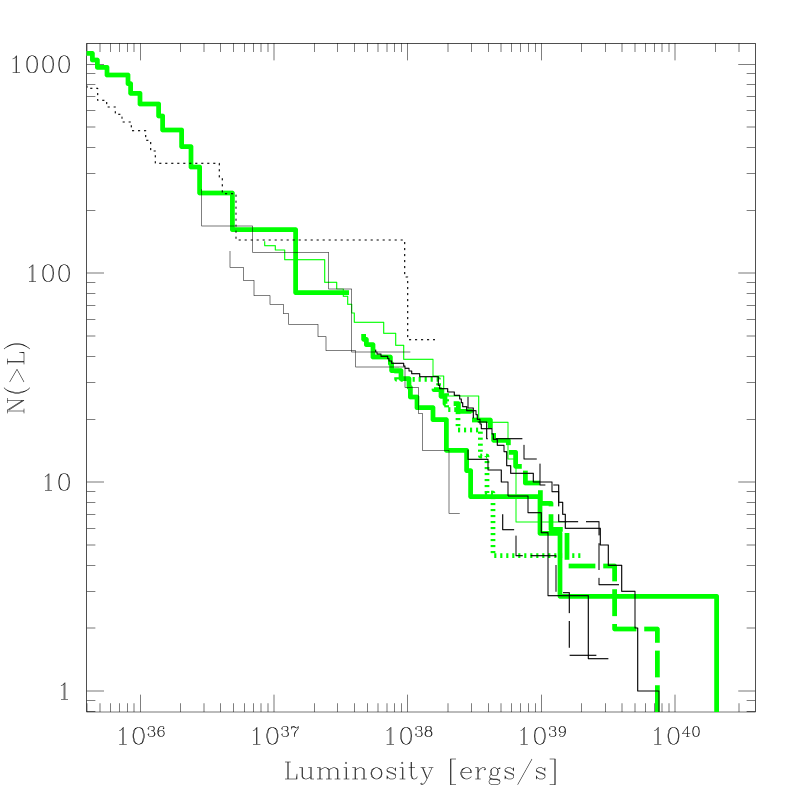
As the next step we compare the luminosity functions of actively star forming galaxies with that of low SFR galaxies. Unfortunately, the X-ray binary population of low SFR galaxies is usually dominated by LMXB systems. One of the cases in which the luminosity function of HMXB sources can be reliably obtained is the Milky Way galaxy, for which all sufficiently bright X-ray binaries are optically identified. Another case is the Small Magellanic Cloud, which has a SFR value similar to our Galaxy, but is $\sim 300-500$ less massive and, correspondingly, has very few, if any, LMXB sources (Yokogawa et al., 2000). Moreover, the SMC is close enough to have optical identifications of HMXBs which makes a distinction like in the Milky Way possible. In order to do the comparison, we combined the luminosity functions of all actively star forming galaxies from our sample with a completeness limit lower than $2\cdot 10^{38}$ erg s^-1 – M 82, Antennae, NGC 4579, NGC 4736 and Circinus. These galaxies have a total SFR of $\sim$ 16 M_⊙ yr^-1, which exceeds the Milky Way SFR ($\sim 0.25$ M_⊙ yr^-1) by a factor of $\sim 65$. Fig. 5 shows the combined luminosity function of the above mentioned star forming galaxies and the luminosity functions of Galactic and SMC HMXBs scaled according to the ratios of SFRs. Shown in Fig. 5 by a solid line is the fit to the luminosity function of the high SFR galaxies only (see below), extrapolated to lower luminosities. It is obvious that the luminosity functions of Galactic and SMC HMXBs agree surprisingly well with an extrapolation of the combined luminosity function of the starburst galaxies.

Thus we demonstrated that the presently available data are consistent with the assumption that the approximate shape and normalisation of the luminosity function for HMXBs in a galaxy with a known star formation rate can be derived from a “universal” luminosity function whose shape is fixed and whose normalisation is proportional to star formation rate. Due to a number of uncertainties involved, the accuracy of this approximation is difficult to assess. Based on our sample of galaxies we can conclude that it might be accurate within $\sim$ 50 per cent.

In order to obtain the universal luminosity function of HMXBs we fit the combined luminosity function of M 82, Antennae, NGC 4579, NGC 4736 and Circinus using a Maximum-Likelihood method with a power law with a cut-off at $L_{c}=2.1\cdot 10^{40}$ erg s^-1 and normalise the result to the combined SFR of the galaxies. The best fit luminosity function (solid line in Fig.5) in the differential form is given by:

$$\frac{dN}{dL_{38}}=(3.3^{+1.1}_{-0.8})\cdot SFR\cdot L_{38}^{-1.61\pm 0.12}\text{~{}~{}for }L<L_{c},$$ (6)

where $L_{38}=L/10^{38}$ erg s^-1 and SFR is measured in units of M_⊙ yr^-1. The errors are $1\sigma$ estimates for one parameter of interest. The rather large errors for normalisation are due to the correlation between slope and normalisation of the luminosity function, with a higher value of normalisation corresponding to a steeper slope. The cumulative form of the luminosity function, corresponding to the best values of the slope and normalisation is:

$$N(>L)=5.4\cdot SFR\cdot(L_{38}^{-0.61}-210^{-0.61}),$$ (7)

According to a Kolmogorov-Smirnov test the data are consistent with the best fit model at a confidence level of 90 per cent.

As an additional test we checked all individual luminosity functions against our best fit using a Kolmogorov-Smirnov test. Taking into account the respective completeness limits, the shapes of all individual luminosity functions are compatible with the assumption of a common ’origin’. In Fig. 6 we show the individual luminosity functions along with the universal luminosity function given by Eq.(6) with the normalisation determined according to the corresponding star formation rates derived from the conventional SFR indicators (Table 1).

Finally, we construct the differential luminosity function combining the data for all galaxies from the primary sample, except for NGC 3256 (having somewhat uncertain completeness limit). To do so we bin all the sources above the corresponding completeness limits in logarithmically spaced bins and normalise the result by the combined SFR of all galaxies contributing to a given bin. Such a method has the advantage of using all the available data. A disadvantage is that due to significantly different luminosity ranges of the individual luminosity functions (especially SMC and Milky Way on one side and star forming galaxies on the other) uncertainties in the conventional SFR estimates may lead to the appearance of artificial features in the combined luminosity function. With that in mind, we plot the differential luminosity function in the right panel of Fig. 5 along with the best fit power law from Eq.(6).

In order to investigate the influence of systematic uncertainties in SFR and distance we performed a Monte-Carlo simulation taking into account these two effects. The grey area in the right panel of Fig. 5 shows the 90 per cent confidence interval obtained from this simulation. In the simulation we randomly varied the distances of galaxies, assuming the errors on the distance to be distributed according to a Gaussian with a mean of 0 and a width of 20 per cent of the distance of a galaxy which corresponds to an uncertainty in luminosity of $\sim$ 40 per cent. Correspondingly the SFR, affected in the same way as the X-ray luminosity by uncertainties in the distance, was changed. Additionally the SFR was randomly varied also assuming a Gaussian error distribution with a mean of 0 and a width of 30 per cent of the SFR, as assumed for Fig. 3. For the Milky Way we varied in each Monte-Carlo run the distance to each HMXB independently with a Gaussian with a mean of 0 and a width of 20 per cent of the distance.

Noteworthy is the fact that the luminosity function is sufficiently close to a single slope power law in a broad luminosity range covering more than five orders of magnitude. If the absence of significant features is confirmed this allows to constrain the relative abundance of NS and BH binaries and/or the properties of accreting compact objects at supercritical accretion rates (see discussion in Sec. 4.1).

However, it should be emphasised that there is hardly any overlap in the luminosity functions for low and high SFR galaxies, as is obvious from Fig. 1 and 5. It happens that this gap is around the Eddington luminosity of a NS, $L_{Edd,NS}$, which should be a dividing line between NS and BH binaries. From simple assumptions it would be expected that the luminosity functions below $L_{Edd,NS}$ are dominated by NS whereas above $L_{Edd,NS}$ BH binaries should dominate. This would imply a break in the luminosity function around $L_{Edd,NS}$ because of different abundances of NSs and BHs. Due to the uncertainties in SFR measurements it is possible that a break, that would theoretically be expected around $L_{Edd,NS}$, could be hidden by this gap. Even upper limits (not more than twice) are of importance and could give some additional information about the relative strength of the two populations of accreting binaries (see discussion in Sec. 4). Observations of star forming galaxies with sufficient sensitivity, i.e. with a completeness limit well below $10^{38}$ erg s^-1 will be able to resolve this question.

3.2 High Luminosity cut-off

The combined luminosity function shown in the left panel of Fig. 5 indicates a possible presence of a cut-off at $L_{c}\sim 2\cdot 10^{40}$ erg s^-1. From a statistical point of view, when analysing the combined luminosity function of the high SFR galaxies only, the significance of the cut-off is not very high, with a single slope power law with slope 0.74 for the cumulative luminosity function also giving an acceptable fit, although with a somewhat lower probability of 54 per cent according to a Kolmogorov–Smirnov test. However, an independent strong evidence for the existence of a cut-off around $\sim{\rm few}\cdot 10^{40}$ erg s^-1 is provided by the $L_{X}$–SFR relation as discussed in the next subsections.

The existence of such a cut-off, if it is real and if it is a universal feature of the HMXB luminosity function, can have significant implications to our understanding of the so-called ultra-luminous X-ray sources. Assuming that these very luminous objects are intermediate mass BHs accreting at the Eddington limit, the value of the cut-off gives an upper limit on the mass of the black hole, $\sim 100$ M_⊙. These apparently super-Eddington luminosities can also be the result of other effects, like a strong magnetic field in NSs which may allow radiation to escape without interacting with the accreting material (Basko & Sunyaev, 1976), emission from a supercritical accretion disk (Shakura & Sunyaev, 1973; Paczynsky & Wiita, 1980), beamed emission (King et al., 2001), or the emission of a jet as suggested by Körding et al. (2002). Moreover, in BHs in high state radiation is coming from the quasi-flat accretion disk where electron scattering gives the main contribution to the opacity. It is easy to show that the radiation flux perpendicular to the plane of the disk exceeds the average value by up to 3 times (Shakura & Sunyaev, 1973). Also the Eddington luminosity is dependent on chemical abundance which allows a twice higher luminosity for accretion of helium. These last two effects alone can provide a factor of 6 above the canonical Eddington luminosity.

It should be mentioned that, based on the combined luminosity function only, we can not exclude the possibility that the cut-off is primarily due to the Antennae galaxies which contributes about half of the sources above $10^{39}$ erg s^-1 and shows a prominent cut-off in its luminosity function. On the other hand, further indication for a cut-off is provided by the luminosity function of NGC 3256. Conventional star formation indicators give a value of SFR of $\sim$ 45 M_⊙ yr^-1, however its luminosity function also shows a cut-off at $\sim 10^{40}$ erg s^-1. Unfortunately, due to the large distance (35 Mpc) and a comparatively short exposure time of the CHANDRA observation, $\sim$ 28 ks, the luminosity function of NGC 3256 becomes incomplete at luminosities shortly below the brightest source and therefore does not allow for a detailed investigation.

3.3 Total X-ray luminosity as SFR indicator

CHANDRA and future X-ray missions with angular resolution of the order of $\sim 1^{\prime\prime}$ would be able to spatially resolve X-ray binaries only in nearby galaxies ($d\la\sim 50-100$ Mpc). For more distant galaxies only the total luminosity of a galaxy due to HMXBs can be used for X-ray diagnostics of star formation.

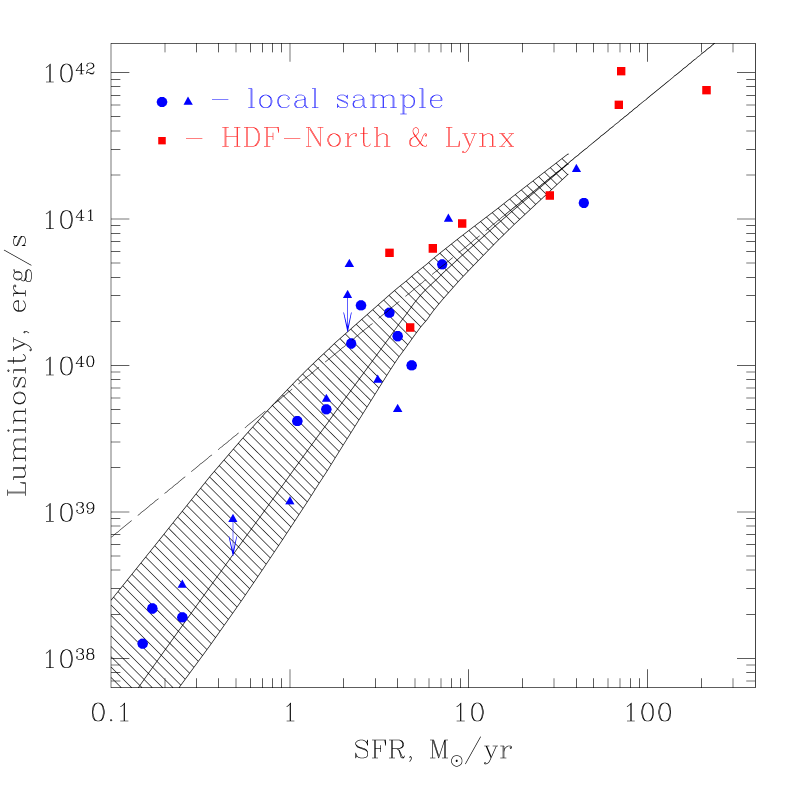
Fig. 7 shows the total luminosity of X-ray binaries (above $10^{36}$ erg s^-1) plotted versus SFR. The galaxies from the primary sample (listed in Table 1) are shown by filled circles. The galaxies, for which only total luminosity is available (Table 2) are shown as filled triangles. The luminosities of the galaxies from the primary sample were calculated by summing the luminosities of individual sources down to the completeness limit of the corresponding luminosity function. The contribution of the sources below the completeness limit was approximately accounted for by integrating a power law distribution with slope $1.6$ and normalisation obtained from the fit to the observed luminosity function. Note, that due to the shallow slope of the luminosity function the total luminosity depends only weakly on the lower integration limit.

As an additional data point we take luminosity and SFR for the Large Magellanic Cloud. The SFR is similar to the Milky Way SFR (Holtzman et al., 1999). Since no luminosity function is presently available for LMC we estimated its integrated X-ray luminosity as a sum of the time averaged luminosities of the three brightest HMXB sources (LMC X-1, X-3, X-4) as measured by ASM (Grimm et al., 2002), $L_{2-10~{}\text{keV}}\approx 3.4\cdot 10^{38}$ erg s^-1. Contribution of the weaker sources should not change this estimate significantly, since the luminosity of the next brightest source is by a factor of $\sim 30-50$ smaller (Sunyaev et al., 1990).

3.4 Theoretical $\bf L_{X}$–SFR relation

At first glance, the relation between collective luminosity of HMXBs and SFR can be easily derived integrating Eq. (6) for the SFR dependent luminosity function. Therefore, as the population of HMXB sources in a galaxy is directly proportional to SFR, one might expect that the X-ray luminosity of galaxies due to HMXB, $L_{X}$, should be linearly proportional to SFR. However this problem contains some subtleties related to the statistical properties of the power law luminosity distribution of discrete sources which appear not to have been recognised previously (at least in astrophysical context). The difference between the most probable value of the total luminosity of HMXB sources in a galaxy (the mode of the distribution) and the ensemble average value (expectation mean, obtained by integrating Eq. (6)) results in the non-linear $L_{X}$–SFR dependence in the low SFR regime. As this effect might be of broader general interest and might work in many different situations related to computing/measuring integrated luminosity of a limited number of discrete objects, we give it a more detailed and rigorous discussion in a separate paper (Gilfanov et al., 2002), and restrict the discussion here to only a brief explanation and an approximate analytical treatment. A somewhat similar problem was considered by Kalogera et al. (2001) in the context of pulsar counts and the faint end of the pulsar luminosity function.

For illustration only, let us consider a population of discrete sources with a Gaussian luminosity function. As is well known, in this case the sum of their luminosities – the integrated luminosity of the parent galaxy, also obeys a Gaussian distribution for which the mean luminosity and dispersion can be computed straightforwardly. An essential property of this simple case is that for an ensemble of galaxies, each having a population of such sources, the most probable value of the integrated luminosity of an arbitrarily chosen galaxy (the mode of the distribution) equals to the mean luminosity (averaged over the ensemble of galaxies). The situation might be different in the case of a population of discrete sources with a power law (or similarly skewed) luminosity function. In this case an ensemble of galaxies would have a non-Gaussian probability distribution of the integrated luminosity. Due to skewness of the probability distribution in this case, the most probable value of the integrated luminosity of an arbitrarily chosen galaxy does not necessarily coincide with the mean value (the ensemble average). The effect is caused by the fact that depending on the slope of the luminosity function and its normalisation the integrated luminosity of the galaxy might be defined by a small number of brightest sources even when the total number of sources is large. Of course, in the limit of large number of sources in the high luminosity end of the luminosity function the distribution becomes asymptotically close to Gaussian and, correspondingly, the difference between the most probable value and the ensemble average vanishes. In this limit the relation between the integrated luminosity of HMXBs and SFR can be derived straightforwardly integrating Eq.(6) for $L_{c}=2.1\cdot 10^{40}$ erg s^-1:

$$L_{X}=6.7\cdot 10^{39}\cdot SFR\text{[M${}_{\odot}$ yr${}^{-1}$]}\text{~{}~{}erg s${}^{-1}$}$$ (8)

It should be emphasised that the ensemble average integrated luminosity (i.e. averaged over many galaxies with similar SFR) is always described by the above equation, independent of the number of sources and shape of the luminosity function. This equality is maintained due to the outlier galaxies, whose luminosity exceeds significantly both the most probable and average values. These outlier galaxies will result in enhanced and asymmetric dispersion in the low SFR-regime.

The following simple consideration leads to an approximate analytical expression for the most probable value of the integrated luminosity. Assuming a power law luminosity function $dN/dL=A\cdot SFR\cdot~{}L^{-\alpha}$ with $1<\alpha<2$, one might expect, that the brightest source would most likely have a luminosity $L_{max}$ close to the value $\sim L_{1}$ such that $N(>L_{1})\sim 1$, i.e.

$$L_{1}\propto SFR^{\frac{1}{\alpha-1}}$$ (9)

In the presence of a cut-off $L_{c}$ in the luminosity function, the luminosity of the brightest source, of course, can not exceed the cut-off luminosity: $L_{max}=\text{min}(L_{1},L_{c})$. The most probable value of the total luminosity can be computed integrating the luminosity function from $L_{min}$ to $L_{max}=\text{min}(L_{1},L_{c})$:

$$L_{total}=\int^{\text{min}(L_{1},L_{c})}_{L_{min}}\frac{dN}{dL}L~{}dL,$$ (10)

which leads to

$$L_{total}\approx\frac{A\cdot SFR}{2-\alpha}\cdot\text{min}(L_{1},L_{c})^{2-\alpha}$$ (11)

for $1<\alpha<2$ and $L_{1},L_{c}>>L_{min}$.

Obviously there are two limiting cases of the $L_{X}$–SFR dependence of the total luminosity on SFR, depending on the relation between $L_{c}$ and $L_{1}$, i.e. on the expected number of sources in the high end of the luminosity function, near its cut-off. In the limit of low SFR (small number of sources) $L_{1}<L_{c}$ and the luminosity of the brightest source would increase with SFR: $L_{max}\sim L_{1}\propto SFR^{\frac{1}{\alpha-1}}$. Therefore the $L_{X}$–SFR dependence might be strongly non-linear:

$$L_{total}\propto SFR^{\frac{1}{\alpha-1}}$$ (12)

e.g. for $\alpha=1.5$ the relation is quadratic $L_{total}\propto SFR^{2}$. For sufficiently large values of SFR $L_{1}>L_{c}$, i.e. $N(>L_{c})>1$ implying a large number of sources in the high luminosity end of the luminosity function and, correspondingly, Gaussian probability distribution of the integrated luminosity. In this case $L_{max}\sim L_{c}=const$ and does not depend on SFR anymore and the dependence is linear, in accord with Eq.(8).

Figure 7: The $L_{X}$–SFR relation. The filled circles and triangles are nearby galaxies from Table 1 (primary sample) and Table 2 (secondary sample), the open circles are distant star forming galaxies from the HDF North and Lynx field. The arrows are the upper limits for the X-ray luminosity due to HMXBs for IC 342 and NGC 891. The thick solid line shows the expected relation between SFR and the most probable value of the total luminosity computed for the best fit parameters of the HMXB luminosity function (exact calculation, from Gilfanov et al. (2002)). Note, that in the low SFR regime the probability to find a galaxy below the solid curve is $\sim 10-15$ per cent. The shaded area shows the 68 per cent confidence region including both intrinsic variance of the $L_{X}$–SFR relation and uncertainty of the best fit parameters of the HMXB luminosity function (Eq.(6)). The dashed line shows the linear $L_{X}$–SFR relation given by Eq.(8).

Importantly, the entire existence of the linear regime in the $L_{X}$–SFR relation is a direct consequence of the existence of a cut-off in the luminosity function. For a sufficiently flat luminosity function, $1<\alpha<2$, the collective luminosity of the sources grows faster than linear because brighter and brighter sources define the total luminosity as the star formation rate increases. Only in the presence of the maximum possible luminosity of the sources, $L_{c}$ (for instance Eddington limit for NSs) the regime can be reached, when $N(>L_{c})$ becomes larger than unity and subsequent increase of the star formation rate results in the linear growth of the total luminosity. The latter, linear, regime of the $L_{X}$–SFR relation was studied independently by Ranalli et al. (2002) based on ASCA and Beppo-SAX data. Note that their equation (12) agrees with our Eq.(8) within 15 per cent.

The position of the break in the $L_{X}$–SFR relation depends on the slope of the luminosity function and the value of the cut-off luminosity:

$${\rm SFR}_{\rm break}\propto L_{c}^{\alpha-1}$$ (13)

Combined with the slope of the $L_{X}$–SFR relation in the low SFR regime (Eq.(12)) and the normalisation of the linear dependence in the high SFR limit this opens a possibility to constrain the parameters of the luminosity function studying the $L_{X}$–SFR relation alone, without actually constructing luminosity functions, e.g. in distant unresolved galaxies.

Table 4: Sample galaxies from the Hubble Deep Field North and Lynx Field

Source	redshift	$F_{1.4~{}GHz}$	SFR	$S_{0.5-8~{}keV}$	$L_{X}$
		[$\mu$Jy]	[M⊙ yr-1]	[$10^{-15}$ erg s-1 cm-2]	[$10^{40}$ erg s-1]
123634.5+621213	0.458	233	28	0.43	14.4
123634.5+621241	1.219	230	213	0.3	75.9
123649.7+621313	0.475	49	8	0.15	2.5
123651.1+621030	0.410	95	9	0.3	9.3
123653.4+621139	1.275	66	69	0.22	60.6
123708.3+621055	0.423	45	4	0.18	5.9
123716.3+621512	0.232	187	5	0.18	1.8
084857.7+445608	0.622	320	71	1.46	102

3.5 $\bf L_{X}$–SFR relation: comparison with the data

The solid line in Fig.7 shows the result of the exact calculation of the $L_{X}$–SFR relation from Gilfanov et al. (2002). The relation was computed for the best fit parameters of the HMXB luminosity function determined from the analysis of five mostly well studied galaxies from the primary sample (section 3.1 and Eq.(6)). Note, that due to the skewness of the probability distribution for $L_{total}$ in the non-linear, low SFR regime the theoretical probability to find a galaxy below the most probable value (the solid curve in Fig.7) is $\approx 12-16$ per cent at SFR = 0.2-1.5 M_⊙ yr^-1 and increases to $\approx$ 30 per cent at SFR = 4-5  M_⊙ yr^-1, near the break of the $L_{X}$–SFR relation. In the linear regime (SFR $\ga 10$ M_⊙ yr^-1) it asymptotically approaches $\sim 50percent$, as expected. The shaded area around the solid curve corresponds to the 68 per cent confidence level including both intrinsic variance of the $L_{X}$–SFR relation and uncertainty of the best fit parameters of the HMXB luminosity function (Eq.(6)).

Fig.7 demonstrates sufficiently good agreement between the data and the theoretical $L_{X}$–SFR relation. Importantly, the predicted relation agrees with the data both in the high and low SFR regime, thus showing that the data, including the high redshift galaxies from Hubble Deep Field North (see the following subsection), are consistent with the HMXB luminosity function parameters, derived from significantly fewer galaxies than plotted in Fig.7.

The existence of the linear part at SFR $>$ 5-10 M_⊙ yr^-1 gives an independent confirmation of the reality of the cut-off in the luminosity function of HMXBs (cf. Sec. 3.2). The position of the break and normalisation of the linear part in the $L_{X}$–SFR relation confirms that the maximum luminosity of the HMXB sources (cut-off in the HMXB luminosity function) is of the order of $L_{c}\sim 10^{40}-10^{41}$ erg s^-1 (see Gilfanov et al. (2002) for more details). Despite the number of theoretical ideas being discussed, the exact reason for the cut-off in the HMXB luminosity function is not clear and significant variations of $L_{c}$ among galaxies, related or not to the galactic parameters, such as metalicity or star formation rate can not be excluded a priori. However, significant variations in $L_{c}$ from galaxy to galaxy would result in large dispersion in the break position and in the linear part of the $L_{X}$–SFR relation. As such large dispersion is not observed, one might conclude that there is no large variation of the cut-off luminosity between galaxies and, in particular, there is no strong dependence of the cut-off luminosity on SFR.

3.6 Hubble Deep Field North

In order to check whether the correlation, which is clearly seen from Fig. 7 for nearby galaxies, holds for more distant galaxies as well we used the data of the CHANDRA observation of the Hubble Deep Field North (Brandt et al., 2001). We cross-correlated the list of the X-ray sources detected by CHANDRA with the catalogue of radio sources detected by VLA at 1.4 GHz (Richards, 2000). Using optical identifications of Richards et al. (1998) and redshifts from Cohen et al. (2000) we compiled a list of galaxies detected by CHANDRA and classified as spiral or irregular/merger galaxies by Richards et al. (1998) and not known to show AGN activity. The K-correction for radio luminosity was done assuming a power law spectrum and using the radio spectral indices from Richards (2000). The X-ray luminosity was K-corrected and transformed to the 2–10 keV energy range using photon indices from Brandt et al. (2001). The final list of galaxies selected is given in Table 4. An additional data point, X-ray flux and redshift, is taken from the observation of the Lynx Field by Stern et al. (2002). The radio flux is obtained from a cross-correlation of the X-ray positions with Oort (1987).

The star formation rates were calculated assuming that the non-thermal synchrotron emission due to electrons accelerated in supernovae dominates the observed 1.4 GHz luminosity and using the following relation from Condon (1992):

$$SFR_{radio}=1.9\cdot 10^{-29}\cdot\nu_{\text{G}Hz}^{\alpha}\cdot L_{\nu}\text{[erg s${}^{-1}$ Hz${}^{-1}$]},$$ (14)

where $\alpha$ is the slope of the non-thermal radio emission.

The galaxies from HDF North and Lynx are shown in Fig.7 by open circles. A sufficiently good agreement with the theoretical $L_{X}$–SFR relation is obvious.

4 Discussion

4.1 Neutron stars, stellar mass black holes and intermediate mass black holes

Two well known and one possible types of accreting objects should contribute to the X-ray luminosity function of sources in star forming galaxies:

1. neutron stars (M $\sim$ 1.4 M_⊙),

2. stellar mass black holes ($3\leq M/M_{\odot}\leq 20$) born due to collapse of high mass stars, and

3. intermediate mass ($50\la M/M_{\odot}\la 10^{5}$) black holes of unknown origin.

Each class of accreting objects is expected to have a maximum possible luminosity, close or exceeding by a factor of several the corresponding Eddington luminosity. In a general case we should expect that each of these three types of accreting objects should have its own luminosity function depending on the mass distribution inside each class (more narrow for NSs, more broad for BHs and probably very broad for intermediate mass BHs), properties of the binary and mass loss type and rate from the normal star. Therefore, the combined luminosity function of a galaxy, containing all three types of objects should have several breaks or steps (see Fig. 8) which are not present in Fig. 5. Such breaks should be connected with the fact that, for example, below the Eddington limit for a NS (or at somewhat higher luminosity) more abundant NS X-ray binaries might dominate in the number of objects, whereas at higher luminosities only black holes should contribute due to their higher masses and broader mass distribution. Until now CHANDRA data did not show any evidence for a break in the luminosity function expected in the vicinity or above of Eddington luminosity for NS mass. However, such a break must exist, the only question is how pronounced and broad it is.

It is believed that stars with masses higher than 60-100 $M_{\odot}$ are unstable. Therefore there should be an upper limit on the mass of BHs born as a result of stellar collapse. Until now the most massive known stellar mass BH in our Galaxy, GRS 1915+105, has a mass of $\sim$15 M_⊙ (Greiner et al., 2001). It is natural that the Eddington luminosity of these objects, amplified several times by angular distribution of radiation and chemical abundance effects, should result in the maximum luminosity of X-ray sources of this type. It is important to mention that 3 years of RXTE/ASM observations revealed from time to time super-Eddington luminosities of some Galactic X-ray binaries on the level of 3–12 $L_{Edd,NS}$ (Grimm et al., 2002).

The hypothetical intermediate mass BHs, probably reaching masses of $\sim 10^{2-5}M_{\odot}$, might be associated with extremely high star formation rates (BHs merging in dense stellar cluster etc.) and are expected to be significantly less frequent than $\sim$stellar mass BHs. Therefore the transition from the $\sim$stellar mass BH HMXB luminosity function to intermediate mass BHs should be visible in the cumulative luminosity function. Merging BHs are one possible way of rapid growth of super-massive BHs that exist in practically all galaxies. To accrete efficiently intermediate mass BHs should form close binary systems with normal stars or be in dense molecular clouds.

If the cut-off in the luminosity function, observed at $\sim$ few $10^{40}$ erg s^-1 corresponds to the maximum possible luminosity of $\sim$stellar mass BHs and if at $L>L_{c}$ the population of hypothetical intermediate mass BHs emerges, it should lead to a drastic change in the slope of the $L_{X}$–SFR relation at extreme values of SFR (Gilfanov et al., 2002). Therefore, observations of distant star forming galaxies with very high SFR might be one of the best and easiest ways to probe the population of intermediate mass black holes.

4.1.1 Three component luminosity function

Figure 8: The upper main figure shows the contributions of neutron stars (thin solid line), stellar (dashed line) and intermediate (dot-dashed line) mass BHs to the differential luminosity function. The thick grey solid line is the total differential luminosity function. For details of the parameters see discussion in the text. The figure in the lower left shows the luminosity around the Eddington limit for a NS. The luminosity functions shown include the simplest assumption that all systems with accretion rates above Eddington radiate at the Eddington luminosity (bottom), two effects allowing super-Eddington luminosities (middle), and additionally a 20 per cent uncertainty in the distance estimate (top). The curves are scaled for clarification. The figure in the lower right shows the luminosity around the Eddington limits for 3–20 M_⊙ BHs. The luminosity functions shown include no effect (bottom), and two effects allowing super-Eddington luminosities (middle) and additionally a 20 per cent uncertainty in the distance estimate (top). The dotted lines denote the uncertainty due to SFR of a factor of 2.

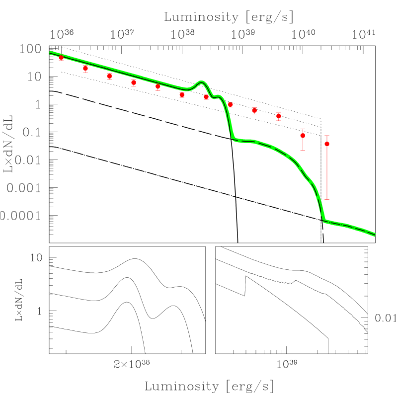
In Fig. 8 we present the result of a simple picture of what type of universal luminosity function a very simple model of HMXB population synthesis could produce. This picture is obviously oversimplified but we present it here to show that the simple picture cannot reproduce the smooth luminosity function we get from CHANDRA observations of star forming galaxies.

The initial set-up includes parameterisation of the mass distributions of NSs and BHs, the distribution of mass transfer rates in binary systems, and a prescription for the conversion of mass transfer rates to X-ray luminosities.

The probability distribution of NS masses was chosen to be a Gaussian distribution with a mean of 1.4 M_⊙ and a $\sigma$ of 0.2 M_⊙. The mass distribution of BHs was chosen to be a power law with a slope of 1.1. These numbers are similar to results of theoretical computations performed by Fryer & Kalogera (2001). The mass distribution for BHs is bimodal, for stellar mass black holes it ranges from 3–20 M_⊙, and secondly, we include intermediate mass BHs ranging from $10^{2}-10^{5}$ M_⊙. We made the simple assumption that their mass distribution has the same slope as for stellar mass BHs.

Normalisations for the probability distributions were chosen such that the number of stellar mass BHs is a factor of 20 smaller than the number of NSs. This is roughly the ratio observed for HMXBs in our Galaxy (Portegies Zwart & Yungelson, 1998; Iben et al., 1995; Grimm et al., 2002). However the ratio of stars with $M>25M_{\odot}$, BH progenitors, to stars with $25M_{\odot}>M>8M_{\odot}$, NS progenitors, is close to 1/2 according to the Salpeter IMF. Therefore in principle the stellar mass BH curve in Fig. 8 might be much closer to the NS curve. The number of intermediate mass BHs is assumed to be a factor of 100 less than the number of stellar mass BHs in HMXBs.

The probability distribution of mass transfer rates in binary systems is set to be a power law with a slope of -1.6, reproducing the observed luminosity function of HMXBs assuming a linear relation between luminosity and mass accretion rate. The limits are 0.1 to $10^{7}$ in units of $10^{16}$ g s^-1. Mass transfer was assumed to be conservative over the whole range, i.e. no mass is lost from the system except for super-Eddington sources and wind accretion. The formulae for conversion of mass accretion rate to X-ray luminosity are

$$L=\eta\cdot\dot{M}_{accretion}\cdot c^{2},$$ (15)

where $\eta=0.1$ for BHs and $\eta=0.15$ for NSs. The mass loss rate from the normal star has no strict limit, however the X-ray luminosity reaches a maximum at the Eddington luminosity and objects with much higher mass accretion rate will end up at the Eddington luminosity introducing a peak in the luminosity function.

For illustration we present two sub-figures in Fig. 8 to show the evolution from sharp features to a smoother curve with the introduction of smearing effects on the luminosity which is shown in the main part of the figure. The first effect is He-accretion when the HMXB is fed by a helium rich star which we take to be the case in about 10 per cent of the sources. Secondly, in the case of BHs a quasi-flat accretion disk with an electron scattering atmosphere (Sobolev, 1949; Chandrasekhar, 1950) radiates according to $(1+2.08\cdot\cos(i))\cos(i)$ where $i$ is the inclination angle, producing 2.6 times higher flux in the direction perpendicular to the disk plane than average (Shakura & Sunyaev, 1973). Sunyaev & Titarchuk (1985) confirmed that this ratio is similar or higher for radiation comptonized in the accretion disk. For slim disks (Paczynsky & Wiita, 1980) this ratio should be even higher. Moreover to demonstrate the influence of distance uncertainties we assumed a variation in distances of 20 per cent. All these effects together give a considerably smoother curve and permit up to 6 times higher luminosities.

These are only the most simple effects that permit to surpass the Eddington limit. Of course other more sophisticated models like jet emission (Körding et al., 2002) or beamed emission (King et al., 2001) or models taking into account strong magnetic fields in X-ray pulsars (Basko & Sunyaev, 1976) also can be employed to explain the observed luminosity function.

4.1.2 Wind driven accreting systems

Our experience with HMXBs in our Galaxy and LMC shows that in many sources accretion happens via capture from a strong stellar wind (Cen X-3, Cyg X-1, 4U 1700+37, 4U 0900-40, and possibly SMC X-1, LMC X-1 and LMC X-4) As we see the majority of Galactic HMXBs are fed by stellar wind accretion. There is a very important difference between wind accretion onto NSs and BHs. The capture radius, $r_{capture}=\frac{2GM}{v_{0}^{2}}$, is proportional to the mass of the accreting object and therefore in similar systems BHs should have $M^{2}$ times larger accretion rates than NSs for the same wind parameters. The dependence of the Roche geometry on the mass ratio make the dependence on M_BH a little weaker.

$$\dot{M}_{capture}\propto\dot{M}_{wind}\cdot(\frac{M_{BH}}{M_{NS}})^{\beta},$$ (16)

where $\beta$ is between 1.5 and 2. This reason might increase the relative BH contribution to the luminosity function in star forming galaxies. It is important that

$$\frac{\dot{M}_{capture}\cdot\eta\cdot c^{2}}{L_{Edd}}\propto\dot{M}_{wind}\cdot M_{BH}^{\beta-1}.$$ (17)

For $\beta>1$ it is preferable for BHs to have higher luminosities than for NSs.

4.1.3 Comparison of simulated and observed luminosity function

The discrepancy between the observed luminosity function in the right panel of Fig. 5 and our simple model in Fig. 8 is obvious. We do not see features in the observed differential luminosity function in the vicinity of $L_{Edd}$ for NSs, neither a peak $\frac{\Delta L}{L}\sim O(2)$ nor a sharp decline at $L>L_{Edd}$ as in the model luminosity function. Furthermore our model luminosity function lacks sources in the luminosity range $10^{39}-10^{40}$ erg s^-1. It seems we should assume that accreting stellar mass BHs in star forming regions are more abundant than in the Milky Way.

It is important to note that having all our corrections we are getting objects close to the limit of maximum luminosity of the observed luminosity functions.

In Fig. 8 is plotted the total accretion luminosity whereas CHANDRA observes only in the range from 1–10 keV. However X-ray pulsars emit the bulk of their luminosity in the range from 20–40 keV. This effect may further decrease the importance of the peak at $2\cdot 10^{38}$ erg s^-1. Since in elliptical galaxies old X-ray binaries with weak magnetic fields, thus having much softer spectra than X-ray pulsars, should dominate the population one should expect the importance of the peak to be larger in ellipticals.

Our simple analysis demonstrates how difficult it is to construct a very smooth luminosity function with the same slope over a broad luminosity range, $10^{35}-10^{40}$ erg s^-1, and without sharp features in the vicinity of Eddington luminosities. Because so many different processes are involved in different parts of this huge luminosity range. Our universal luminosity function based on CHANDRA, ASCA and RXTE data has no strong features. The absence of features around the Eddington luminosity for NSs should be explained but it is also necessary to explain the absence of the abrupt change in the luminosity function at higher luminosities when less numerous BHs dominate the luminosity function.

The most obvious shortcomings of this naive model are the mass distributions of BHs and NSs, the normalisations for BHs, especially for intermediate mass BHs, and the assumptions of conservative mass transfer and that all super-Eddington sources radiate at Eddington luminosity in X-rays. It is also very difficult to assume that intermediate mass BHs form a continuous mass function with stellar mass BHs without a strong break around 20–50 M_⊙. They should have their own luminosity function with different normalisation and slope. Another problem is connected with the formation of binaries with normal stars feeding intermediate mass BHs and making them bright X-ray sources. The observation of HMXBs in other galaxies will allow to put constraints on the combination of these parameters.

The main concern with with the existence of a featureless universal luminosity function (ULF) is connected with the interpretation of the following experimental facts:

• RXTE/ASM, ASCA and CHANDRA give us information about the low luminosity part of the ULF ($L_{X}\la 10^{38}$ erg s^-1) based on the Milky Way, SMC and NGC 1569.

• CHANDRA data on the other galaxies in Table 1 give information about the high luminosity part of the ULF ($L_{X}\ga 10^{38}$ erg s^-1).

• UV, FIR and radio methods of SFR determination in both local and more distant samples of galaxies have significant systematic uncertainties, see Table 3.

To resolve these uncertainties arising very close to the Eddington luminosity for a NS we need to additional data permitting to get the slope of the luminosity function in Antennae-type galaxies at luminosities significantly below $10^{38}$ erg s^-1. Furthermore we need to increase the sample of nearby galaxies where we can extend the luminosity function well above $10^{38}$ erg s^-1. Only this will give full confidence that there is no change in the normalisation in the ULF near $10^{38}$ erg s^-1.

4.2 Further astrophysically important information

The good correlation between SFR and total X-ray luminosity due to HMXBs and the total number of HMXBs can obviously become a powerful and independent way to measure SFR in distant galaxies. In addition, this correlation is providing us with further astrophysically important information:

• These data are showing that NSs and BHs are produced in star forming regions very efficiently and in very short time, confirming the main predictions of stellar evolution.

• The luminosity function of HMXBs does not seem to depend strongly on the trigger of the star formation event which might be completely different for the Milky Way and e.g. the Antennae where it is the result of tidal interaction of two galaxies.

• The good agreement of the X-ray luminosity – SFR relation of HDF galaxies with the theoretical prediction proves that the HMXB formation scenario at high redshifts does not differ significantly from nearby HMXB formation.

• The luminosity function provides information that neutron stars and BHs have a similar distribution of accretion rates in all galaxies of the sample available for study today.

• The luminosity function of HMXBs does not seem to depend strongly on the chemical abundances in the host galaxy.

• The existence of well separated X-ray sources is a way to look for small satellites of massive galaxies, like SMC.

The integral X-ray luminosity and X-ray source counts are unique sources of information on binaries in distant galaxies. Other methods of investigation of SFR (UV, IR, radio) rely on the luminosity distribution and number of the brightest stars, without a significant dependence on the amount of binaries in a high mass star population. On the other hand the existence of an observed population of HMXBs in another galaxy is possible only in the case if there are conditions for formation of close binaries with certain mass loss from a normal companion and efficient capture of out-flowing stellar wind or Roche lobe overflow by an accreting object. Detailed observations of X-ray sources in our own Galaxy have shown how small the allowed parameter space is – this is the reason why the number of X-ray sources in the Galaxy is so small (Illarionov & Sunyaev, 1975) in comparison with the total number of NSs and BHs and the total number of O and B stars. Therefore:

• The existence of a universal luminosity function of HMXBs proves that the formation of close massive X-ray binaries and their distribution on mass ratio, separation and mass exchange rate is similar in all regions of active star formation up to redshifts z$\sim$1.

5 Conclusion

Based on CHANDRA and ASCA observations of nearby star forming galaxies and RXTE/ASM, ASCA, and MIR-KVANT/TTM data on our Galaxy and the Magellanic Clouds we studied the relation between star formation and the population of high mass X-ray binaries. Within the accuracy and completeness of the data available at present, we conclude that:

1. The data are broadly consistent with the assumption that in a wide range of star formation rates the luminosity distribution of HMXBs in a galaxy can be approximately described by a universal luminosity function, whose normalisation is proportional to the SFR (Fig. 1, 4, 5). Although the accuracy of this approximation is yet to be determined based on a larger galaxy sample and deeper observations, we conclude from the rather limited sample available, that it might be of the order of $\sim$50 per cent or better.

   In differential form the universal luminosity function can be approximated as a power law with a cut-off at $L_{c}\sim 2\cdot 10^{40}$ erg s^-1:

   $$\frac{dN}{dL_{38}}=(3.3^{+1.1}_{-0.8})\cdot SFR\cdot L_{38}^{-1.61\pm 0.12}\text{~{}~{}for }L<L_{c},$$ (18)

   where SFR is measured in units of M_⊙ yr^-1 and $L_{38}=L/10^{38}$ erg s^-1. In cumulative form it is correspondingly:

   $$N(>L_{38})=(5.4^{+2.1}_{-1.7})\cdot SFR\cdot(L_{38}^{-0.61\pm 0.12}-210^{-0.61\pm 0.12}).$$ (19)

   Although more subtle effects can not presently be excluded (and are likely to exist), we did not find strong non-linear dependences of the HMXB luminosity function on SFR. We neither found strong dependences of the HMXB luminosity function on other parameters of the host galaxy, such as metalicity or star formation trigger.

2. Both the number and total luminosity of HMXBs in a galaxy are directly related to the star formation rate and can be used as an independent SFR indicator.

3. The total number of HMXBs is directly proportional to SFR (Fig. 3):

   $$\text{SFR [M${}_{\odot}$ yr${}^{-1}$]}=\frac{N(L>2\cdot 10^{38}\text{erg s${}^{-1}$})}{2.9}.$$ (20)

4. The dependence of the total X-ray luminosity of a galaxy due to HMXBs on SFR has a break at SFR $\approx$ 4.5 M_⊙ yr^-1 for $M>8$ M_⊙.

   At sufficiently high values of star formation rate, SFR$\ga 4.5$ M_⊙ yr^-1 ($L_{\rm 2-10~{}keV}\ga 3\cdot 10^{40}$ erg s^-1 correspondingly) the X-ray luminosity of a galaxy due to HMXBs is directly proportional to SFR (Fig.7):

   $${\rm SFR}[{\rm M}_{\odot}{\rm yr}^{-1}]=\frac{L_{\rm 2-10~{}keV}}{6.7\cdot 10^{39}{\rm erg~{}s}^{-1}}$$ (21)

   At lower values of the star formation rate, SFR$\la 4.5$ M_⊙ yr^-1 ($L_{\rm 2-10~{}keV}\la 3\cdot 10^{40}$ erg s^-1), the $L_{X}-SFR$ relation is non-linear: (Fig.7):

   $${\rm SFR}[{\rm M}_{\odot}{\rm yr}^{-1}]=\left(\frac{L_{\rm 2-10~{}keV}}{2.6\cdot 10^{39}{\rm erg~{}s}^{-1}}\right)^{0.6}$$ (22)

   The non-linear $L_{X}-SFR$ dependence in the low SFR limit is not related to non-linear SFR dependent effects in the population of HMXB sources. It is rather caused by non-Gaussianity of the probability distribution of the integrated luminosity of a population of discrete sources. We will give this a more detailed and rigorous treatment in a forthcoming paper (Gilfanov et al., 2002).

5. Based on the data of CHANDRA observations of the Hubble Deep Field North we showed, that the relation (21) between the SFR and the X-ray luminosity of a galaxy due to HMXBs holds for distant star forming galaxies with redshifts as high as $z=1.2$ (Fig. 7).

6. The good agreement of high redshift observations with theoretical predictions and the fact that X-ray observations exclusively rely on the binary nature of the sources is evidence that not only the amount of star formation at redshifts up to $\sim$1 can be easily obtained from the above relations but also that the HMXB formation scenario is very similar at least up to this redshift.

7. The entire existence of the linear regime in the $L_{X}$–SFR relation is a direct consequence of the existence of a cut-off in the luminosity function. The position of the break in the $L_{X}-SFR$ relation depends on the cut-off luminosity $L_{c}$ in the luminosity function of HMXB as SFR${}_{\rm break}\propto L_{c}^{\alpha-1}$, where $\alpha$ is the differential slope of the luminosity function. Combined with the slope of the $L_{X}$–SFR relation in the low SFR regime (Eq.(12)) this opens a possibility to constrain the parameters of the luminosity function studying the $L_{X}$–SFR relation alone, without actually constructing the luminosity functions, e.g. in distant unresolved galaxies.

   Agreement of the predicted $L_{X}-SFR$ relation with the data both in high and low SFR regime (Fig.7) gives an independent evidence of the existence of a cut-off in the luminosity function of HMXBs at $L_{c}\sim{\rm several}\times 10^{40}$ erg s^-1. It also indicates that $L_{X}-SFR$ data, including the high redshift galaxies from Hubble Deep Field North, are consistent with the HMXB luminosity function parameters, derived from significantly fewer galaxies, than plotted in Fig.7.

References

- Armus et al. (1990) Armus L., Heckman T. M., Miley G. K., 1990, \apj, 364, 471
- Awaki et al. (2002) Awaki H., Matsumoto H., Tomida H., 2002, \apj, 567, 892
- Bahcall (1983) Bahcall J. N., 1983, \apj, 267, 52
- Basko & Sunyaev (1976) Basko M. M., Sunyaev R. A., 1976, \mnras, 175, 395
- Bell & Kennicutt (2001) Bell E. F., Kennicutt R. C., 2001, \apj, 548, 681
- Bolton (1972) Bolton C. T., 1972, Nature Physical Science, 240, 124+
- Brandt et al. (2001) Brandt W. N., Alexander D. M., Hornschemeier A. E., Garmire G. P., Schneider D. P., Barger A. J., Bauer F. E., Broos P. S., Cowie L. L., Townsley L. K., Burrows D. N., Chartas G., Feigelson E. D., Griffiths R. E., Nousek J. A., Sargent W. L. W., 2001, \aj, 122, 2810
- Brinchmann & Ellis (2000) Brinchmann J., Ellis R. S., 2000, \apjl, 536, L77
- Buat et al. (2002) Buat V., Boselli A., Gavazzi G., Bonfanti C., 2002, \aap, 383, 801
- Chandrasekhar (1950) Chandrasekhar S., 1950, Radiative transfer.. Oxford, Clarendon Press, 1950.
- Cohen et al. (2000) Cohen J. G., Hogg D. W., Blandford R., Cowie L. L., Hu E., Songaila A., Shopbell P., Richberg K., 2000, \apj, 538, 29
- Condon (1992) Condon J. J., 1992, \araa, 30, 575
- Condon et al. (1990) Condon J. J., Helou G., Sanders D. B., Soifer B. T., 1990, \apjs, 73, 359
- David et al. (1992) David L. P., Jones C., Forman W., 1992, \apj, 388, 82
- de Vaucouleurs et al. (1991) de Vaucouleurs G., de Vaucouleurs A., Corwin H. G., Buta R. J., Paturel G., Fouque P., 1991, Third Reference Catalogue of Bright Galaxies. Volume 1-3, XII, 2069 pp. 7 figs.. Springer-Verlag Berlin Heidelberg New York
- Eneev et al. (1973) Eneev T. M., Kozlov N. N., Sunyaev R. A., 1973, \aap, 22, 41+
- Eracleous et al. (2002) Eracleous M., Shields J. C., Chartas G., Moran E. C., 2002, \apj, 565, 108
- Fabbiano (1994) Fabbiano G., 1994, X-ray binaries. Cambridge University Press, p. 390
- Fabbiano et al. (1988) Fabbiano G., Gioia I. M., Trinchieri G., 1988, \apj, 324, 749
- Feitzinger (1980) Feitzinger J. V., 1980, Space Science Reviews, 27, 35
- Fryer & Kalogera (2001) Fryer C. L., Kalogera V., 2001, \apj, 554, 548
- Galletta & Recillas-Cruz (1982) Galletta G., Recillas-Cruz E., 1982, \aap, 112, 361
- Georgakakis et al. (2000) Georgakakis A., Forbes D. A., Norris R. P., 2000, \mnras, 318, 124
- Ghosh & White (2001) Ghosh P., White N. E., 2001, \apjl, 559, L97
- Gilfanov et al. (2002) Gilfanov M., Grimm H.-J., Sunyaev R., 2002, Collective luminosity of a population of discrete sources: Astrophysical implications, in preparation
- Gonzalez Delgado & Perez (1996) Gonzalez Delgado R. M., Perez E., 1996, \mnras, 281, 1105
- Greiner et al. (2001) Greiner J., Cuby J. G., McCaughrean M. J., 2001, \nat, 414, 522
- Griffiths et al. (2000) Griffiths R., Ptak A., Feigelson E., Garmire G., Townsley L., Brandt W., Sambruna R., Bregman J., 2000, Science, 290, 1325
- Griffiths & Padovani (1990) Griffiths R. E., Padovani P., 1990, \apj, 360, 483
- Grimm et al. (2002) Grimm H.-J., Gilfanov M., Sunyaev R., 2002, \aap, 391, 923
- Holtzman et al. (1999) Holtzman J. A., Gallagher J. S., Cole A. A., Mould J. R., Grillmair C. J., Ballester G. E., Burrows C. J., Clarke J. T., Crisp D., Evans R. W., Griffiths R. E., Hester J. J., Hoessel J. G., Scowen P. A., Stapelfeldt K. R., Trauger J. T., Watson A. M., 1999, \aj, 118, 2262
- Hoopes et al. (2001) Hoopes C. G., Walterbos R. . M., Bothun G. D., 2001, \apj, 559, 878
- Huchtmeier & Richter (1988) Huchtmeier W. K., Richter O.-G., 1988, \aap, 203, 237
- Iben et al. (1995) Iben I. J., Tutukov A. V., Yungelson L. R., 1995, \apjs, 100, 217
- Illarionov & Sunyaev (1975) Illarionov A. F., Sunyaev R. A., 1975, \aap, 39, 185
- Israel (1988) Israel F. P., 1988, \aap, 194, 24
- Körding et al. (2002) Körding E., Falcke H., Markoff S., 2002, \aap, 382, L13
- Kaaret (2001) Kaaret P., 2001, \apj, 560, 715
- Kalogera et al. (2001) Kalogera V., Narayan R., Spergel D. N., Taylor J. H., 2001, \apj, 556, 340
- Karachentsev et al. (1997) Karachentsev I., Drozdovsky I., Kajsin S., Takalo L. O., Heinamaki P., Valtonen M., 1997, \aaps, 124, 559
- Kennicutt (1998) Kennicutt R. C., 1998, \araa, 36, 189
- Kennicutt et al. (1994) Kennicutt R. C., Tamblyn P., Congdon C. E., 1994, \apj, 435, 22
- Kilgard et al. (2001) Kilgard R. E., Kaaret P. E., Krauss M. I., McDowell J. C., Prestwich A. H., Raley M. T., Zezas A., 2001, American Astronomical Society Meeting
- King et al. (2001) King A., Davies M., Ward M., Fabbiano G., Elvis M., 2001, ApJ, 552, L109
- Kuno & Nakai (1997) Kuno N., Nakai N., 1997, \pasj, 49, 279
- Lípari et al. (2000) Lípari S., Díaz R., Taniguchi Y., Terlevich R., Dottori H., Carranza G., 2000, \aj, 120, 645
- Lehnert & Heckman (1996) Lehnert M. D., Heckman T. M., 1996, \apj, 472, 546+
- Lira et al. (2002) Lira P., Ward M., Zezas A., Alonso-Herrero A., Ueno S., 2002, \mnras, 330, 259
- Liu & Kennicutt (1995) Liu C. T., Kennicutt R. C., 1995, \apj, 450, 547+
- Lyutyi et al. (1973) Lyutyi V. M., Syunyaev R. A., Cherepashchuk A. M., 1973, Soviet Astronomy, 17, 1+
- Madau & Pozzetti (2000) Madau P., Pozzetti L., 2000, \mnras, 312, L9
- Martin et al. (2002) Martin C. L., Kobulnicky H. A., Heckman T. M., 2002, \apj, 574, 663
- Moshir et al. (1993) Moshir M., Copan G., Conrow T., McCallon H., Hacking P., Gregorich D., Rohrbach G., Melnyk M., Rice W., Fullmer L., 1993, VizieR Online Data Catalog, 2156, 0
- Negishi et al. (2001) Negishi T., Onaka T., Chan K.-W., Roellig T. L., 2001, \aap, 375, 566
- Oort (1987) Oort M. J. A., 1987, \aaps, 71, 221
- Paczynsky & Wiita (1980) Paczynsky B., Wiita P., 1980, A&A, 88, 23
- Persic & Salucci (1988) Persic M., Salucci P., 1988, \mnras, 234, 131
- Portegies Zwart & Yungelson (1998) Portegies Zwart S. F., Yungelson L. R., 1998, \aap, 332, 173
- Ptak et al. (2001) Ptak A., Griffiths R., White N., Ghosh P., 2001, \apjl, 559, L91
- Ranalli et al. (2002) Ranalli P., Comastri A., Setti G., 2002, The 2–10 keV luminosity as a star formation rate indicator, astro-ph/0202241
- Reakes (1980) Reakes M., 1980, \mnras, 192, 297
- Rephaeli & Gruber (2002) Rephaeli Y., Gruber D., 2002, \aap, 389, 752
- Rice et al. (1988) Rice W., Lonsdale C. J., Soifer B. T., Neugebauer G., Koplan E. L., Lloyd L. A., de Jong T., Habing H. J., 1988, \apjs, 68, 91
- Richards (2000) Richards E. A., 2000, \apj, 533, 611
- Richards et al. (1998) Richards E. A., Kellermann K. I., Fomalont E. B., Windhorst R. A., Partridge R. B., 1998, \aj, 116, 1039
- Roberts et al. (2002) Roberts T., Warwick R., Ward M., Murray S., 2002, A Chandra observation of the interacting pair of glaaxies NGC 4485/NGC 4490, astro-ph/0208196
- Rosa-Gonzalez et al. (2002) Rosa-Gonzalez D., Terlevich E., Terlevich R., 2002, An Empirical Calibration of Star Formation Rate Estimators, accepted by MNRAS
- Roussel et al. (2001) Roussel H., Sauvage M., Vigroux L., Bosma A., 2001, \aap, 372, 427
- Rownd & Young (1999) Rownd B. K., Young J. S., 1999, \aj, 118, 670
- Sage (1993) Sage L. J., 1993, \aap, 272, 123
- Sandage & Tammann (1980) Sandage A., Tammann G. A., 1980, A revised Shapley-Ames Catalog of bright galaxies. Washington: Carnegie Institution, 1980, Preliminary version
- Schreier et al. (1972) Schreier E., Giacconi R., Gursky H., Kellogg E., Tananbaum H., 1972, \apjl, 178, L71
- Schurch et al. (2002) Schurch N., Roberts T., Warwick R., 2002, High-resolution X-ray imaging and spectroscopy of the core of NGC 4945 with XMM-Newton and Chandra, astro-ph/0204361
- Shakura & Sunyaev (1973) Shakura N., Sunyaev R., 1973, \aap, 24, 337
- Sharina et al. (1996) Sharina M. E., Karachentsev I. D., Tikhonov N. A., 1996, \aaps, 119, 499
- Smith & Wilson (2001) Smith D. A., Wilson A. S., 2001, \apj, 557, 180
- Sobolev (1949) Sobolev V., 1949, Seria Matem. Nauk, 18, N1163
- Sofue et al. (1992) Sofue Y., Reuter H.-P., Krause M., Wielebinski R., Nakai N., 1992, \apj, 395, 126
- Soria & Kong (2002) Soria R., Kong A. K. H., 2002, \apjl, 572, L33
- Soria & Wu (2002) Soria R., Wu K., 2002, \aap, 384, 99
- Spinoglio et al. (1995) Spinoglio L., Malkan M. A., Rush B., Carrasco L., Recillas-Cruz E., 1995, \apj, 453, 616
- Stern et al. (2002) Stern D., Tozzi P., Stanford S. A., Rosati P., Holden B., Eisenhardt P., Elston R., Wu K. L., Connolly A., Spinrad H., Dawson S., Dey A., Chaffee F. H., 2002, \aj, 123, 2223
- Strickland et al. (2001) Strickland D. K., Colbert E. J. M., Heckman T. M., Weaver K. A., Dahlem M., Stevens I. R., 2001, \apj, 560, 707
- Sunyaev et al. (1990) Sunyaev R., Gilfanov M., Churazov E., Loznikov V., Yamburenko N., Skinner G. K., Patterson T. G., Willmore A. P., Emam O., Brinkman A. C., Heise J., Intzand J., Jager R., 1990, Soviet Astronomy Letters, 16, 55+
- Sunyaev et al. (1978) Sunyaev R. A., Tinsley B. M., Meier D. L., 1978, Comments on Astrophysics, 7, 183
- Sunyaev & Titarchuk (1985) Sunyaev R. A., Titarchuk L. G., 1985, \aap, 143, 374
- Tananbaum et al. (1972) Tananbaum H., Gursky H., Kellogg E., Giacconi R., Jones C., 1972, \apjl, 177, L5
- Terashima & Wilson (2002) Terashima Y., Wilson A., 2002, Ultraluminous X-ray sources in M51, astro-ph/0204321
- Thronson et al. (1989) Thronson H. A., Hunter D. A., Casey S., Harper D. A., Latter W. B., 1989, \apj, 339, 803
- Toomre & Toomre (1972) Toomre A., Toomre J., 1972, \apj, 178, 623
- Ueda et al. (2001) Ueda Y., Ishisaki Y., Takahashi T., Makishima K., Ohashi T., 2001, \apjs, 133, 1
- Verbunt & van den Heuvel (1994) Verbunt F., van den Heuvel E., 1994, X-ray binaries. Cambridge University Press, p. 457
- Viallefond et al. (1980) Viallefond F., Allen R. J., de Boer J. A., 1980, \aap, 82, 207
- Wilkinson & Evans (1999) Wilkinson M. I., Evans N. W., 1999, \mnras, 310, 645
- Yokogawa et al. (2000) Yokogawa J., Imanishi K., Tsujimoto M., Nishiuchi M., Koyama K., Nagase F., Corbet R. H. D., 2000, \apjs, 128, 491
- Young et al. (1996) Young J. S., Allen L., Kenney J. D. P., Lesser A., Rownd B., 1996, \aj, 112, 1903
- Zezas et al. (2002) Zezas A., Fabbiano G., Rots A., Murray S., 2002, Chandra observations of ”The Antennae” galaxies (NGC4038/39): II. Detection and analysis of galaxian X-ray sources, astro-ph/0203174