XMM-Newton and Chandra Observations of the Galaxy Group NGC 5044.
I. Evidence for Limited Multi-Phase Hot Gas

Abstract

Using new XMM and Chandra observations we present an analysis of the temperature structure of the hot gas within a radius of 100 kpc of the bright nearby galaxy group NGC 5044. A spectral deprojection analysis of data extracted from circular annuli reveals that a two-temperature model (2T) of the hot gas is favored over single-phase or cooling flow ($\hbox{{$\dot{M}$}}=4.5\pm 0.2$ $M_{\sun}$ yr^-1) models within the central $\sim 30$ kpc. Alternatively, the data can be fit equally well if the temperature within each spherical shell varies continuously from $\sim\hbox{{$T_{\rm h}$}}$ to $\hbox{{$T_{\rm c}$}}\sim\hbox{{$T_{\rm h}$}}/2$, but no lower. The high spatial resolution of the Chandra data allows us to determine that the temperature excursion $\hbox{{$T_{\rm h}$}}\rightarrow\hbox{{$T_{\rm c}$}}$ required in each shell exceeds the temperature range between the boundaries of the same shell in the best-fitting single-phase model. This is strong evidence for a multiphase gas having a limited temperature range. We do not find any evidence that azimuthal temperature variations within each annulus on the sky can account for the range in temperatures within each shell. We provide a detailed investigation of the systematic errors on the derived spectral models considering the effects of calibration, plasma codes, bandwidth, variable $N_{\rm H}$, and background rate. We find that the RGS gratings and the EPIC and ACIS CCDs give fully consistent results when the same models are fitted over the same energy ranges for each instrument. The cooler component of the 2T model has a temperature ($\hbox{{$T_{\rm c}$}}\sim 0.7$ keV) similar to the kinetic temperature of the stars. The hot phase has a temperature ($\hbox{{$T_{\rm h}$}}\sim 1.4$ keV) characteristic of the virial temperature of the $\sim 10^{13}$ $M_{\odot}$ halo expected in the NGC 5044 group. However, in view of the morphological disturbances and X-ray holes visible in the Chandra image within $R\approx 10$ kpc, bubbles of gas heated to $\sim\hbox{{$T_{\rm h}$}}$ in this region may be formed by intermittent AGN feedback. Some additional heating at larger radii may be associated with the evolution of the cold front near $R\sim 50$ kpc, as suggested by the sharp edge in the EPIC images.

1 Introduction

The hot gas in groups and clusters of galaxies is a vital window on the history of star formation and metal enrichment in the Universe. But to discover this history requires first a measurement of the thermodynamic properties of the hot gas in these systems. The temperature structure of the gas is of special importance since it is required to determine quantities such as the entropy and the metal abundances. Galaxy groups are especially well-suited for studies of their temperature structure since their $\sim 1$ keV temperatures occur near the peak in sensitivity of current X-ray CCDs and near the strong, highly temperature-sensitive iron L-shell emission lines.

Using new XMM and Chandra observations we present an analysis of the temperature structure of the hot gas of NGC 5044, perhaps the brightest group in soft X-rays. Although several previous ROSAT and ASCA studies demonstrated that the hot gas within $r\sim 30$ kpc is not isothermal (e.g., David et al., 1994; Buote, 1999), the data could not distinguish between single-phase and multiphase models. The combined spatial and spectral resolution of the XMM and Chandra CCDs allows for unprecedented mapping of the temperatures and elemental abundances of the hot gas in groups and clusters. The higher energy resolution, sensitivity, and larger field-of-view of the XMM EPIC CCDs are better suited for constraining the spatial and spectral properties of the diffuse hot gas out to radii well past the optical extent of the central galaxy; i.e., out to $r\sim 100$ kpc assuming a distance of 33 Mpc using the results of Tonry et al. (2001) for $H_{0}=70$ km s^-1 Mpc^-1 (note: $1\arcsec=0.160$ kpc). The $\sim 1\arcsec$ resolution of Chandra is particularly useful for addressing the properties of the hot gas on smaller scales.

In this paper we analyze the temperature structure of the hot gas in NGC 5044. The metal abundances (Buote et al., 2003b, hereafter Paper 2) and gravitating mass distribution are discussed in companion papers.

2 Observations and Data Preparation

2.1 XMM

NGC 5044 was observed with the EPIC pn and MOS CCD cameras for approximately 20 ks and 22 ks respectively during AO-1 as part of the XMM Guest Observer program. We generated calibrated events lists for the data using the standard SAS v5.3.3 software. Since the diffuse emission of NGC 5044 fills the entire field of view we estimate the background using the standard “background templates”. These templates are events lists obtained by combining several high Galactic latitude pointings.

Inspection of the CCD light curves for events with energies above 10 keV does not reveal any strong flares in the NGC 5044 observation, but there are times of increased activity which are more pronounced in the pn data. After applying the count-rate screening criteria recommended to match the background templates (and also the standard screening criteria recommended for all observations), we arrive at final exposures of 19.5 ks for the MOS1, 19.3 ks for the MOS2, and 8.9 ks for the pn.

Since the quiescent background varies typically by $\sim 10\%$ it is necessary to normalize the background templates to each source observation. Since NGC 5044 has a gas temperature $\sim 1$ keV there is little emission from hot gas for energies $>5$ keV. We renormalized the MOS1 and MOS2 background templates by comparing source and background counts in the 7-12 keV band extracted from regions near the edges of the MOS fields. We obtain background normalizations that are %16 and %5 above nominal respectively for the MOS1 and MOS2.

Since the strict events screening mentioned above leaves the pn with $<50\%$ of its raw exposure, it is evident that background flares contaminate the pn more than the MOS. Even after the strict screening, we still require a background normalization that is 21% above nominal for the pn. Although this fraction is not much larger than for the MOS1, an excess of the source over the background is clearly visible above energies of a few keV. We have therefore also investigated a potentially more accurate method of subtracting the flaring background following our study of the XMM observation of NGC 1399 (Buote et al., 2003a). That is, after subtracting the pn spectra taken from regions near the edge of the field with the standard background templates re-scaled by their nominal exposures, we fitted the resultant spectrum with a two-component model consisting of a thermal component, represented by an apec thermal plasma, and a broken power-law (BPL) model, representing the residual flaring background which is most pronounced at high energies. For the BPL model we obtain a break energy of 0.6 keV with power-law indices of -2.6 below the break and 0.54 above the break; i.e., over most of the bandpass of interest ($>0.6$ keV) the flaring background is well-described by a power-law with index 0.54.

This BPL model defines the shape of the excess background above the standard templates. We determined its normalization separately for each region of interest using data between 6.0 and 7.25 keV. This 6 keV lower limit is selected to avoid contamination from softer source emission while the upper limit is chosen to avoid calibration emission lines. We find that this method to subtract the excess background in the pn data gives results consistent with the simpler method of renormalizing the background template. In this paper we use the BPL model of the excess background as our default method for the pn.

2.2 Chandra

NGC 5044 was observed by Chandra with the ACIS-S3 camera for $\approx 22$ ks during AO-1. The events list was corrected for charge-transfer inefficiency according to Townsley et al. (2002), and only events characterized by the standard ASCA grades were used. The standard ciao software (version 2.2.1) was used for most of the subsequent data preparation.

Since the diffuse X-ray emission of NGC 5044 fills the entire S3 chip, we used the standard background templates to model the background. After running the standard lc_clean script to clean the source events list of flares with the same screening criteria as the background templates, we arrive at a final exposure time of $20.2$ ks for NGC 5044.

3 Image and Radial Profile

Figure 1: (Left panel) False-color mosaic of the XMM MOS1 and MOS2 images of NGC 5044 adaptively smoothed using the SAS task asmooth. The image has been divided by the summed MOS1 and MOS2 exposure maps to correct for exposure variations. (Right panel) Portion of the archival Chandra ACIS-S image (also false-color) located at the center of NGC 5044 adaptively smoothed using the CIAO task csmooth. In both images celestial N is up and E is to the left.

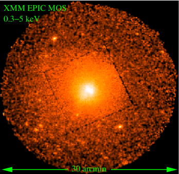
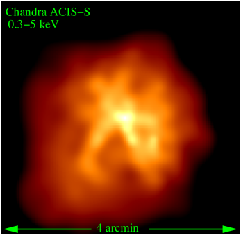
In Figure 1 we display an adaptively smoothed mosaic of the XMM MOS1 and MOS2 images as well as the adaptively smoothed Chandra ACIS-S3 image. Several sources can be seen embedded in the diffuse emission which fills the entire MOS field. That we see more sources at large radius suggests that discrete sources at smaller radii are swamped by the diffuse emission which is brightest near the center. A careful inspection of the MOS and pn images within $R\approx 1\arcmin$ of NGC 5044 reveals significant non-circular features. The higher-resolution Chandra ACIS-S image (Figure 1) shows these features to be holes in the hot gas similar to those seen in Chandra images of the cores of galaxy clusters (e.g., Fabian et al., 2000; McNamara et al., 2000; Churazov et al., 2001). Typically these holes are filled by extended radio emission that emanates from a central source. However, the ($\approx 45\arcsec$) NVSS (Condon et al., 1998) radio image of NGC 5044 reveals only a fairly bright central point-like source suggestive of an AGN. Perhaps a deeper observation at higher resolution would find extended radio emission filling the X-ray holes.

Over a radius $R\approx 1-5\arcmin$ (i.e., to the edge of the central MOS CCD) the diffuse emission is approximately circular with concentric isophotes. Between $R\approx 5-6\arcmin$ the isophote centroid is slightly offset from values at smaller radius. The origin of this shift is apparent in Figure 1 as excess emission to the East and N-E outside the central CCD. This offset was noted previously in the ROSAT PSPC observation of NGC 5044 (David et al., 1994). The XMM image, however, also reveals that there is a sharp edge in the X-ray surface brightness on the West, N-W side near this offset region, $R\sim 6\arcmin$. This type of sharp feature has been observed recently in Chandra observations of several galaxy clusters and has been interpreted as a “cold front”; i.e., a contact discontinuity between regions of different density and temperature (see Markevitch et al., 2002). We note that at radii larger than $\sim 6\arcmin$ the isophote centroids are consistent with those for $R\lesssim 5\arcmin$.

Figure 2: (Left panel) Azimuthally averaged 0.3-5 keV surface brightness profile of the background-subtracted, exposure-corrected combined MOS1 and MOS2 data (kpc units on top axis). The lower points represent the combined background values. The best-fitting $\beta$ model for the MOS data is indicated by the dashed line. (Right panel) Same quantities are plotted for the pn data.

We characterized the image further by computing the azimuthally averaged surface brightness profile in the 0.3-5 keV band separately for the MOS and pn data. We created exposure maps for each detector using the standard SAS software and used these maps to flatten the images. We combined the MOS1 and MOS2 data into a single exposure-corrected image. The same procedures were followed for the background images. (Since here we are not concerned with the detailed spectral dependence of the background for the pn we used the renormalized template accounting for the factor of 21% discussed in §2.) Point sources and chip gaps were masked out from the calculation.

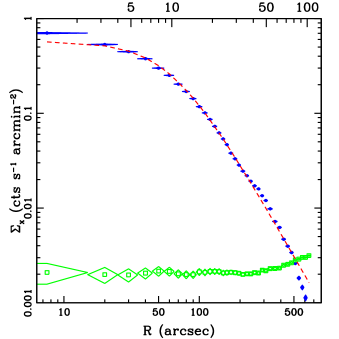
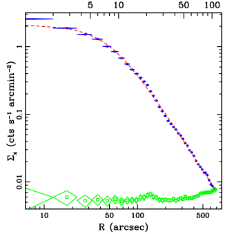
The radial profiles, $\Sigma_{\rm x}(r)$, of the source and background images are shown in Figure 2. Within $R\sim 7\arcmin$ the radial profiles are similar for both detectors, but at larger radii the profiles appear to deviate. To facilitate comparison between the profiles, we fitted standard “$\beta$ models” convolved with the XMM PSF to $\Sigma_{\rm x}(r)$. The best-fitting models are shown in Figure 2. We obtained parameters, $r_{\rm c}=61.9\pm 0.4\arcsec$, and $\beta=0.585\pm 0.001$ for the MOS and, $r_{\rm c}=47.9\pm 0.4\arcsec$, and $\beta=0.522\pm 0.001$ for the pn. The values of these parameters confirm the impression from the figure that at large radius $\Sigma_{\rm x}(r)$ is steeper for the MOS.

The steeper profile of the MOS at larger radii is probably the result of small errors in the background estimate at large radius. Near $R=7\arcmin$ the MOS background rate equals the source rate indicating that the derived $\Sigma_{\rm x}(r)$ for the source is very sensitive to small errors in the background for $R\gtrsim 7\arcmin$. In contrast, the background rate does not equal the source rate for the pn until near the edge of the field, $R\sim 11\arcmin$. The robustness of $\Sigma_{\rm x}(r)$ for the pn is also supported by the analysis of the ROSAT data of NGC 5044 by David et al. (1995) who obtained $\beta=0.53\pm 0.02$ consistent with our result for the pn. If data with $R>400\arcsec$ are excluded for the MOS, then we obtain best-fitting parameters, $r_{\rm c}=52.1\arcsec$ and $\beta=0.542$, in better agreement with the pn and ROSAT values.

We conclude that a single $\beta$ model is a good average description of the radial surface brightness profile of NGC 5044 between $R\sim 10\arcsec$ and $\sim 11\arcmin$. (At the center there is evidence for a small excess above the $\beta$ model on the scale of the PSF. This is also the region where the azimuthal distortions are most pronounced in the Chandra image.) Therefore, the possible “cold front” suggested by the isophotal centroid offset near $R=6\arcmin$ does not substantially distort the radial profile away from that of an equilibrium configuration.

4 Spectral Deprojection Analysis

Motivated by the regular appearance of the radial profile and the lack of substantial azimuthal variations in the spectral properties, we focus our analysis on the azimuthally (and spherically) averaged spectral properties of the X-ray emission. We present an analysis of the azimuthal spectral properties of the Chandra and XMM data in §5.

4.1 Preliminaries

For each XMM detector (MOS1,MOS2,pn) we extracted spectra in concentric circular annuli located at the X-ray centroid of the inner contours (i.e., computed within a $2\arcmin$ radius) such that the width of each annulus contained $\approx 8000$ background-subtracted counts in the 0.3-5 keV band in each MOS detector, and the minimum width was set to $1\arcmin$ for PSF considerations; note that we address residual effects of the PSF by comparison to fits of the high-resolution Chandra data alone in §4.3 and §6. Obvious point sources were masked out before the extraction (and corresponding regions also were omitted from the background templates). These restrictions resulted in a total of eight annuli within $r=10\arcmin$; these annuli are defined in Table 1. (Note that the results we present below are quite insensitive to the choice of radius within which to compute the centroid.) RMF and ARF files were generated using SAS. (Note that the vignetting correction is administered through the ARF file.) Finally, the spectral pulse-invariant (PI) files for each annulus were rebinned such that each energy bin contains a minimum of 30 counts appropriate for $\chi^{2}$ fitting.

We first consider the Chandra data extracted in the same regions as the XMM data subject to the constraint that the regions lie entirely within the ACIS-S3 field. This restriction gives Chandra data within the first three radial bins defined for the XMM data. Later in §4.3 we shall examine the Chandra data within smaller spatial regions. We have applied the latest corrections to the Chandra ARF files that account for a time-dependent degradation in the quantum efficiency at lower energies (i.e., ciao corrarf routine).

To obtain the three-dimensional properties of the X-ray emitting gas we perform a spectral deprojection analysis assuming spherical symmetry using the (non-parametric) “onion-peeling” technique. That is, one begins by determining the spectral model in the bounding annulus and then works inward by subtracting off the spectral contributions from the outer annuli. We have previously developed a code based on xspec (Arnaud, 1996) to implement this procedure (Buote, 2000a). Consequently, we obtain temperatures, abundances, densities, and absorption column densities (and any other desired parameters) by fitting spectral models to the “deprojected spectra”.

In this procedure we account for the emission projected from shells outside of our bounding annulus by assuming the X-ray emissivity for such shells varies as a power-law with radius and has the same spectral shape as determined from the bounding annulus. For the XMM data for NGC 5044 we take the radial surface brightness to vary as $r^{-2}$ (or $\beta=0.5$ for the $\beta$ model) as indicated by the data within $R=10\arcmin$. As found previously (§3.1 of Buote 2000a) the derived spectral parameters (except density in the penultimate annulus) are quite insensitive to this choice.

To estimate the uncertainties on the fitted parameters we simulated spectra for each annulus using the best-fitting models and fit the simulated spectra in exactly the same manner as done for the actual data. From 20 Monte Carlo simulations we compute the standard deviation for each free parameter which we quote as the “$1\sigma$” error. (This is a slightly different manner of quoting the errors compared to §3.2 of Buote 2000a.)

Because deprojection always inflates the errors between points, which is related to the error associated with the derivative of the emissivity in an Abel inversion, we regularize (i.e., smooth) some of the parameters (see §3.3 of Buote 2000a). In actuality we regularize ex post facto by restricting the value of a parameter within certain bounds specified by a pre-determined radial variation for the parameter. We find it necessary to regularize only the O and Ne abundances so that the radial abundance variation of the logarithmic derivative is between $\pm 2$. We emphasize that regularization only applies to O and Ne for the deprojected (3D) spectral analysis. No regularization is applied to any 2D model.

We take the solar abundances in xspec (v11.2.0af) to be those given by the Grevesse & Sauval (1998) table which use the correct new photospheric value for iron which agrees also with the value obtained from solar-system meteorites (e.g., McWilliam, 1997).

4.2 Simultaneous Fitting of XMM-Chandra Data

Table 1: Quality of Spectral Fits ($\chi^{2}$/dof) for 1T and 2T Models

	$R_{\rm in}$	$R_{\rm out}$	1T		2T
Bin	(arcmin)	(arcmin)	2D	3D	2D	3D
1	0.0	0.5	779.8/451	737.9/451	646.7/449	644.0/449
2	0.5	1.5	1812.3/689	1368.1/689	974.2/687	949.8/687
3	1.5	2.5	1338.2/693	1189.0/693	855.3/691	836.0/691
4	2.5	3.5	730.6/482	666.8/482	610.3/480	537.3/480
5	3.5	4.5	535.6/454	504.7/454	521.7/452	484.4/452
6	4.5	5.7	547.7/469	548.3/469	516.2/467	514.4/467
7	5.7	7.6	538.0/515	572.4/515	519.7/513	550.0/513
8	7.6	10.1	674.6/561	674.6/561	658.7/559	658.7/559

Within the eight annuli defined in Table 1 we consider simultaneous fits to the MOS1, MOS2, and pn XMM data within radial bins 4-8 for which we do not have Chandra data. Within radial bins 1-3 we perform simultaneous fits to the Chandra and XMM data. Comparison of the Chandra and XMM data within their overlap regions is discussed in §6. We focus on fits performed over the energy range 0.5-5 keV from consideration of the iron abundances obtained from separate Chandra and XMM fits as discussed in Paper 2. However, all results presented for the temperatures in this paper are consistent with those obtained when fitting 0.3-5 keV (§6).

Our baseline model (1T) consists of a single thermal plasma component using the apec code modified by foreground Galactic absorption ($\hbox{{$N_{\rm H}$}}=5\times 10^{20}$ cm^-2) using the phabs model in xspec. The free parameters for this baseline model are all associated with the plasma component: temperature ($T$), normalization, and Fe, O, Ne, Mg, Si, and S abundances – all other elements tied to Fe in their solar ratios. (Models with intrinsic absorption are discussed in §6.) We obtained results for the 1T model fitted directly to the data projected on the sky (i.e., traditional 2D model) and also fitted to the deprojected data (i.e., 3D model) as discussed in §4.

To account for small calibration differences between detectors we multiplied the spectrum of each detector by a detector-dependent constant. These constants were determined by fitting the 1T model to the data with the constants as free parameters. We fixed the constants to these values for all subsequent spectral fits. This approach guarantees that the relative normalizations of multiple emission components (e.g., in 2T models) are the same for each detector.

4.2.1 Single-Temperature Models

Figure 3: Radial temperature profiles (units – bottom: arcminutes, top: kpc) and $1\sigma$ errors for (Left panel) 1T and (Right panel) 2T models fitted simultaneously to XMM and Chandra data. Note that the Chandra data apply only to the inner three radial bins. In each case “3D” refers to results obtained from a spectral deprojection analysis.

Figure 4: Emission measure of the cooler and hotter components for the 2T (3D) model whose temperatures are plotted in Figure 3. The emission measure is expressed as the normalization of the apec plasma model as given in xspec; i.e., normalization is $10^{-14}n_{e}n_{p}V/(4\pi D_{A}^{2}(1+z)^{2})$, where $n_{e}$ is the electron number density, $n_{p}$ is the proton number density, $V$ is the emitting volume, $D_{A}$ is the angular diameter distance, and $z$ is the redshift. The units are arcminutes on the bottom axis and kpc on the top axis.

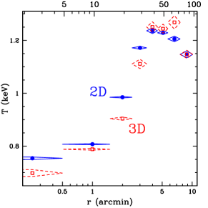
The temperature profiles for the 1T models (2D and 3D) are displayed in Figure 3. For the 1T (2D) model the temperature rises from $T\sim 0.7$ keV at the center to $T\sim 1.2$ keV at large radii consistent with previous 2D ROSAT determinations (e.g., David et al., 1994; Buote, 2000a). The 3D temperature has a steeper rise outward from the center consistent with the 2D profile being smeared by projection effects. The lower temperature in the bounding annulus certainly suggests a declining temperature value, but its value is underestimated because of projection; i.e., we have had to assume the projected emission from shells exterior to our bounding annulus has the same spectral shape as the bounding annulus (§4).

The $\chi^{2}$ values for both models are listed in Table 1. This model is a reasonably good fit in the outer annuli, but the fit degrades at progressively smaller radii, though the trend reverses somewhat for the central annulus. For most radial bins the 2D and 3D fits are similar, with the 3D model usually giving slightly better $\chi^{2}$ values. In shells 2-4, however, the 3D model clearly provides a better fit indicating that annuli 2-4 contain multiple temperature components projected on to the sky.

The 1T (3D) model is still a relatively poor fit in shells 1-4. In Figure 5 we show the EPIC and ACIS spectra for annulus 2 fitted to the 1T (3D) model fits and residuals. The 1T (3D) model yields fit residuals near 1 keV that are fully characteristic of those obtained when trying to force a single-temperature model to fit a spectrum consisting of a multiple components with temperatures near 1 keV (e.g., Buote & Fabian, 1998; Buote, 1999, 2000b). The small deviations above 2 keV also suggest the presence of another (higher) temperature component.

4.2.2 Two-Temperature Models

Since the fits within the central regions – even when the spectral data are deprojected – indicate the presence of at least one more spectral component, we investigated fitting simple two-temperature models (2T) to the data. The abundances for each component are tied together to limit the number of free parameters and because relaxing this condition does not amount to a substantial improvement in the fit quality. (In Paper 2 we briefly discuss 2T models with separately varying abundances on each component.) Consequently, the 2T models add only two free parameters: the temperature and normalization of the second component.

The $\chi^{2}$ values for both the 2T (2D) and 2T (3D) models are listed in Table 1. In all spatial bins the fits are improved by the 2T models, with the greatest improvement occurring in the central bins (1-4). The considerable improvement for bin 2 is shown in Figure 6 for the 2T (3D) model. In comparison to Figure 5 the fit residuals are reduced substantially, and overall the fit is as good as could be expected for such a simple model.

The values of $\chi^{2}$ obtained for the 2T (2D) and 2T (3D) models are very similar, but the 3D models generally have lower $\chi^{2}$ values. Only in bin 4 is the 3D model an obvious improvement over the 2D version. Since 2T models can mimic radial temperature variations accurately, this agreement is not unexpected. Nevertheless, because of the similarity between the 2D and 3D fits, projection effects are not very important for the 2T models.

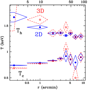
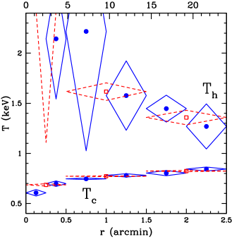
The temperature profiles of the 2D and 3D 2T models are displayed in Figure 3. Focusing for the moment on the 2D model which has better constrained values than the 3D model, it is seen that both the cool ($T_{\rm c}$) and hot ($T_{\rm h}$) temperature components are consistent with an isothermal radial profile for $R\gtrsim 20$ kpc. For smaller radii, $T_{\rm c}$ remains nearly constant with an indication of a slight downturn in the central two bins. The hotter component rises slightly at the center. The values of $T_{\rm c}$ at small radii and the values of $T_{\rm h}$ at large radii are similar to the 1T temperature values.

Within the 1-2 $\sigma$ errors the 3D and 2D temperatures are consistent in all bins, but there are some trends that deserve attention. At large radii ($r\gtrsim 40$ kpc) $T_{\rm c}$ is not tightly constrained particularly for the 3D model; the exception is the final bin where the 2D and 3D fits are equivalent in our deprojection procedure (apart from the inferred normalization). In bin 7 the cooler component is barely detected in 3D; the ratio of normalizations for the best-fitting cooler-to-hotter components is 0.12 for the 2D model compared to only 0.03 for the 3D model. Also in bin 7 the value of $T_{\rm c}$ is poorly constrained for the 3D model, and the best-fitting value of 0.5 keV is located at the lower range we allowed for during the fit. We attribute the stronger detection of the 2T model in bin 8 compared to bin 7 to the limitation in the way we treat the deprojection of the bounding annulus; i.e., our deprojection method assumes the source flux at large radii has the same spectrum as the bounding shell.

At small radius ($r\lesssim 10$ kpc), the temperature of the hotter component rises and becomes poorly constrained in bin 1 for the 3D model, where the best-fitting value is$T=3.7$ keV and the lowest value from 100 Monte Carlo simulations is 1.4 keV which is shown in Figure 3. It is possible that the rise in $T_{\rm h}$ in bin 2, and especially bin 1, arises from the emission of unresolved discrete sources similar to the trend observed for the related system, NGC 1399 (Buote, 2002). If we add a 10 keV bremsstrahlung (brem) component to the 2T models the fits are not improved, but the fitted value of $T_{\rm h}$ in bins 1-2 are consistent with those adjacent bins. Moreover, we obtain a luminosity $\hbox{{$L_{\rm x}$}}\approx 3\times 10^{40}$ erg cm^-2 s^-1 for the brem component. Since this value is comparable to the (relatively uncertain) luminosity expected from discrete sources in NGC 5044 using the results of O’Sullivan et al. (2001), we conclude that the unresolved emission from discrete sources is a viable candidate for the rise in $T_{\rm h}$ at small radius in the 2D models (though $T_{\rm h}$ is still a separate component from the discrete sources).

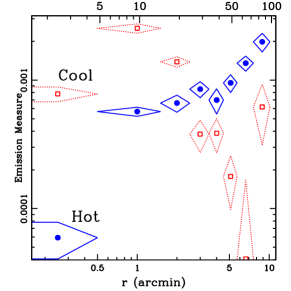
In Figure 4 we plot the emission measures for each component of the 2T (3D) model. The cooler component dominates within $\sim 10$ kpc while the hotter component dominates for $r\gtrsim 50$ kpc. Over $\approx 15-40$ kpc the relative emission measures of the components are within a factor of two of each other.

Figure 5: (Left panel) EPIC MOS1, MOS2, pn, and ACIS-S3 spectra for annulus #2 fitted with a 1T (3D) model. (Right panel) A close-up of the plot in the left panel emphasizing the the MOS and ACIS data and model in the region of strong iron L-shell lines.

Figure 6: (Left panel) Same as Figure 5 except that the 2T (3D) model is shown.

4.2.3 Cooling Flow and Other Multitemperature Models

Table 2: Quality of Spectral Fits ($\chi^{2}$/dof) for other Multitemperature Models

Shell	Cooling Flow	GDEM	PLDEM
1	729.6/450	695.5/450	665.0/449
2	1375.6/688	1091.4/688	973.3/687
3	982.1/692	869.7/692	847.2/691
4	591.2/481	546.5/481	546.9/480
5	490.7/453	484.6/453	494.7/452
6	526.0/468	518.9/468	535.8/467
7	561.1/514	554.3/514	558.1/514
8	659.7/560	658.3/560	660.6/560

Table 3: Selected Parameters for other Multitemperature Models

	Cooling Flow	GDEM		PLDEM
	$\dot{M}$	$T_{0}$	$\sigma_{T}$	$\alpha$	$T_{\rm min}$	$T_{\rm max}-T_{\rm min}$
Shell	($M_{\sun}$ yr-1)	(keV)	(keV)		(keV)	(keV)
1	$0.00\pm 0.15$	$0.72\pm 0.01$	$0.10\pm 0.04$	$-5.0\pm 2.3$	$0.62\pm 0.14$	$>0.5$
2	$3.02\pm 0.13$	$0.83\pm 0.01$	$0.14\pm 0.01$	$-4.6\pm 0.5$	$0.69\pm 0.01$	$>0.7$
3	$0.71\pm 0.07$	$0.94\pm 0.01$	$0.16\pm 0.01$	$-3.9\pm 2.1$	$0.75\pm 0.04$	$1.2\pm 0.6$
4	$0.33\pm 0.05$	$1.22\pm 0.02$	$0.26\pm 0.03$	$0.6\pm 1.6$	$0.72\pm 0.13$	$1.0\pm 0.2$
5	$0.01\pm 0.03$	$1.31\pm 0.05$	$0.19\pm 0.11$	$3.4\pm 4.8$	$1.19\pm 0.30$	$0.1\pm 0.6$
6	$0.14\pm 0.04$	$1.37\pm 0.06$	$0.29\pm 0.14$	$-5.4\pm 3.2$	$1.19\pm 0.28$	$0.1\pm 0.6$
7	$0.04\pm 0.07$	$1.27\pm 0.03$	$0.00\pm 0.04$	0	$1.23\pm 0.35$	$0.1\pm 0.8$
8	$0.22\pm 0.05$	$1.22\pm 0.02$	$0.22\pm 0.04$	0	$0.87\pm 0.27$	$0.7\pm 0.7$

Since the 2T models are preferred over the 1T models (particularly in bins 1-4), we investigated other multitemperature spectral models to attempt to constrain the general differential emission measure (DEM) of the emission spectrum. Because the task of inferring the general DEM from the X-ray spectrum of a coronal plasma is difficult and often highly degenerate (Craig & Brown, 1976), especially for data of only moderate energy resolution such as provided by the XMM and Chandra CCDs, we probed the DEM using a few parameterized models. For this discussion we focus on models fitted to the deprojected spectra; i.e., 3D models.

Cooling Flow: The DEM for an ideal gas cooling at constant pressure from a maximum temperature, $T_{\rm max}$, is (e.g., Johnstone et al., 1992),

$$\xi_{\rm cf}(T)={5\over 2}{\dot{M}k_{B}\over\mu m_{p}}{1\over\Lambda(T)},\hskip 14.22636pt$$ (1)

for $T\leq\hbox{{$T_{\rm max}$}}$. Here $k_{B}$ is Boltzmann’s constant, $m_{p}$ is the proton mass, $\Lambda(T)$ is the plasma emissivity which we take to be given by the apec code, and $\dot{M}$ is the mass drop-out rate. The luminosity of this cooling gas emitted over some energy range $\Delta E$ is,

$$L_{\Delta E}^{\rm cf}=\int^{\hbox{{$T_{\rm max}$}}}_{\hbox{{$T_{\rm min}$}}}\Lambda_{\Delta E}(T)\xi_{\rm cf}(T)dT,$$ (2)

where $\Lambda_{\Delta E}(T)$ is the plasma emissivity integrated over the bandwidth ${\Delta E}$. We set $\hbox{{$T_{\rm min}$}}=0.05$ keV. The total emission spectrum of a cooling flow model is taken to be $L_{\Delta E}^{\rm cf}$ plus the spectrum of a $1T$ model with $T=\hbox{{$T_{\rm max}$}}$ to represent the emission from the ambient gas. We shall refer to this cooling flow model as “CF+1T”. Note that this model adds only one free parameter over the 1T case, i.e., $\dot{M}$, since we tie together the abundances between the two components.

The $\chi^{2}$ values for the CF+1T model fitted to the XMM and Chandra data are listed in Table 2. Although the CF+1T fits are an improvement over the 1T models in some bins, the improvement is not nearly as great as observed for the 2T model. The largest improvement occurs in shells 3-4 where the $\chi^{2}$ values of the CF+1T model are roughly half-way between the 1T and 2T values. The CF+1T model offers no improvement over the 1T model in bins 1-2.

The total mass deposition rate (see Table 3) for all shells (i.e., within $r=97$ kpc) is, $\hbox{{$\dot{M}$}}=4.5\pm 0.2$ $M_{\sun}$ yr^-1. This value is less than half that obtained from the ROSAT imaging analysis of NGC 5044 by David et al. (1994) and only $\approx 1/8$ that obtained from the single-aperture analysis of the ASCA data by Buote (1999). The much smaller value of $\dot{M}$ obtained from the spatially resolved spectral analysis of the XMM and Chandra data is very similar to the reduction obtained from Chandra and XMM results for cooling flow clusters (e.g., David et al., 2001).

In fact, $\dot{M}$ is even slightly smaller because the value in the bounding shell is very likely overestimated. The spike in $\dot{M}$ in shell 8 is almost certainly biased by the edge effect inherent in our deprojection procedure (§4).

Gaussian: An important consideration is whether the better fits obtained by the 2T (3D) model over the 1T (3D) model could simply reflect the range of temperatures within each shell arising from the radially varying temperature profile implied by the 1T fits. In support of this hypothesis is the fact that the improvement of the 2T model is greatest in shells 1-4 where the 1T temperature profile is changing most rapidly with radius; i.e., there we should have the largest range of temperatures per shell.

To test this hypothesis we have explored a model where the temperature distributions within each shell are a Gaussian. The Gaussian DEM (GDEM) is expressed as,

$$\xi_{\rm g}(T)=\frac{norm}{\sigma_{T}\sqrt{2\pi}}\exp\left[-{(T-T_{0})^{2}/2\sigma_{T}^{2}}\right],$$ (3)

where $T_{0}$ is the mean and $\sigma_{T}$ the standard deviation of the Gaussian, and $norm$ is a constant proportional to $n_{e}n_{p}V$ as defined for the apec code in xspec (see caption to Figure 4). The luminosity over some energy range $\Delta E$ is therefore given by equation (2) with $\xi_{\rm g}(T)$ replacing $\xi_{\rm cf}(T)$ and $T_{\rm max}$ and $T_{\rm min}$ set to $\pm\infty$.

In shells 1-4 the GDEM model provides superior fits to the 1T and cooling flow models, but does not have $\chi^{2}$ values quite as low as the 2T model. For example, in shell 3 we obtain for the Gaussian model, $\chi^{2}=869.7$ for 692 dof compared to $\chi^{2}=1189.0$ for 1T, $\chi^{2}=982.1$ for CF+1T, and $\chi^{2}=836.0$ for 2T. Note that the Gaussian adds only $\sigma_{T}$ as a free parameter over the 1T model; i.e., it has the same number of free parameters as the cooling flow model but one less than the 2T model.

The fitted values of $\sigma_{T}$ for shells 5-7 are consistent with the single-phase hypothesis within the $1-1.5\sigma$ errors on $\sigma_{T}$. For shell 8 $\hbox{{$\sigma_{T}$}}=0.22\pm 0.05$ keV could reflect the projection of cooler gas from exterior shells as discussed in §4.2.2 for the 2T models. We cannot determine this for certain with the present data set.

In contrast, in shells 2-4 (and perhaps shell 1) the fitted values of $T_{0}$ and $\sigma_{T}$ do not appear to be consistent with the radially varying single-phase hypothesis. The $1\hbox{{$\sigma_{T}$}}$ ranges for the temperatures of the GDEM model are 0.68-0.97 keV for shell 2, 0.78-1.11 keV for shell 3, 0.95-1.48 keV for shell 4. The considerable overlap of these $1\sigma$ values is in conflict with the small temperature range expected from the single-phase hypothesis. That is, for the 1T (3D) model, the temperature difference between shells 1 and 3 is $0.21\pm 0.01$ keV, between shells 2 and 4 is $0.32\pm 0.02$ keV, and between shells 3 and 5 is $0.35\pm 0.02$ keV. The single-phase hypothesis predicts, therefore, a range of temperatures of approximately half the difference between adjacent shells; i.e., $\approx 0.11$ keV within shell 2, $\approx 0.16$ keV within shell 3, and $\approx 0.17$ keV within shell 4. These values are considerably smaller than the $1\hbox{{$\sigma_{T}$}}$ ranges of $0.28\pm 0.02$ keV for shell 2, $0.32\pm 0.02$ keV for shell 3, and $0.52\pm 0.06$ keV for shell 4.

The temperature difference between shells 1-2 is $0.09\pm 0.01$ keV for the 1T (3D) model implying a single-phase temperature range of $\approx 0.05$ keV. The $1\hbox{{$\sigma_{T}$}}$ range for the GDEM model in shell 1 is $\hbox{{$\sigma_{T}$}}=0.10\pm 0.04$ keV which is only marginally discrepant with the single-phase hypothesis.

Power Law: Finally, to further quantify deviations from the single-phase hypothesis we have investigated spectral fits using a power-law DEM (PLDEM),

$$\xi_{\rm pl}(T)=\begin{cases}{norm\over\log(T_{\rm max}/T_{\rm min})}T^{\alpha},&\alpha=-1\\[5.0pt] {norm(\alpha+1)\over(T_{\rm max}^{\alpha+1}-T_{\rm min}^{\alpha+1})}T^{\alpha},&\alpha\neq-1\\ \end{cases}$$ (4)

where $norm$ is a constant proportional to $n_{e}n_{p}V$ as defined for the apec code in xspecas discussed previously (see caption to Figure 4. The luminosity over some energy range $\Delta E$ is therefore given by equation (2) with $\xi_{\rm pl}(T)$ replacing $\xi_{\rm cf}(T)$. This model adds two free parameters over the 1T model: $\alpha$ and the width of the temperature distribution, $\hbox{{$T_{\rm max}$}}-\hbox{{$T_{\rm min}$}}$; i.e., the power-law model has the same number of free parameters as the 2T model. Because the values of $\alpha$ and $\hbox{{$T_{\rm max}$}}-\hbox{{$T_{\rm min}$}}$ are correlated we found it necessary to restrict their values during the fits to $-5\leq\alpha\leq 5$ and $\hbox{{$T_{\rm max}$}}-\hbox{{$T_{\rm min}$}}\leq 10$ keV.

As indicated in Table 2, the PLDEM model fits nearly as well as the 2T model in every shell. Because $\alpha$ is not well constrained, particularly at larger radii, we fixed $\alpha\equiv 0$ in in shells 7-8. Even with this restriction, the power-law model fits nearly as well as the 2T model in those shells.

The results obtained for $\alpha$, $T_{\rm min}$, and $\hbox{{$T_{\rm max}$}}-\hbox{{$T_{\rm min}$}}$ are listed in Table 3. Like both the 2T and GDEM models, in shells 5-7 there is little indication of significant multitemperature gas; i.e., $\hbox{{$T_{\rm min}$}}\gtrsim 1.2$ keV and $\hbox{{$T_{\rm max}$}}-\hbox{{$T_{\rm min}$}}$ is small (though uncertain). Similarly, in shell 8 the PLDEM model indicates the presence of multiple temperature components which likely arises from projection of gas exterior to shell 8 (see §4.2.2).

For shells 1-4 the PLDEM fits imply a substantial range of temperature components in each shell. In shell 4 we have $\alpha\approx 0$ which indicates an equal contribution from temperature components over a range from approximately 0.7 keV to 1.7 keV (with some uncertainty in the upper limit). The value of $\alpha$ becomes increasingly negative at smaller radius showing that the temperature distribution is progressively more peaked near $T_{\rm min}$. However, the large values of $\hbox{{$T_{\rm max}$}}-\hbox{{$T_{\rm min}$}}$ reflect the rise in $T_{\rm h}$ seen for the 2T models at lower radius which is probably attributed to the emission from unresolved stellar sources (§4.2.2).

Overall, the PLDEM model, like the 2T and GDEM models, indicate that within shells 1-4 the temperature distribution is too wide within each shell to be described by a radially varying single-phase medium. The XMM CCD data cannot distinguish between the PLDEM and 2T models; i.e., a continuous versus a discrete temperature distribution.

4.3 Smaller Regions with Chandra

Table 4: $\chi^{2}$/dof for Selected Models Fitted Only to the Chandra Data

	$R_{\rm in}$	$R_{\rm out}$
Shell	(arcmin)	(arcmin)	1T	2T	GDEM
1C	0.00	0.25	100.7/65	94.1/63	98.3/64
2C	0.25	0.50	130.9/85	95.7/83	118.2/84
3C	0.50	1.00	177.1/116	122.4/114	149.1/115
4C	1.00	1.50	196.5/120	129.4/118	141.5/119
5C	1.50	2.00	235.1/118	159.1/116	164.7/117
6C	2.00	2.50	170.1/116	138.9/114	148.0/115

Table 5: Parameters for Selected Models Fitted Only to the Chandra Data

	1T	2T		GDEM
	$T$	$T_{\rm c}$	$T_{\rm h}$	$T_{0}$	$\sigma_{T}$
Shell	(keV)	(keV)	(keV)	(keV)	(keV)
1C	$0.61\pm 0.04$	$0.61\pm 0.03$	$\cdots$	$0.63\pm 0.11$	$0.15\pm 0.14$
2C	$0.73\pm 0.03$	$0.70\pm 0.03$	$2.1\pm 0.6$	$0.77\pm 0.05$	$0.23\pm 0.08$
3C	$0.75\pm 0.01$	$0.75\pm 0.01$	$2.2\pm 1.2$	$0.76\pm 0.01$	$0.11\pm 0.05$
4C	$0.79\pm 0.01$	$0.78\pm 0.02$	$1.58\pm 0.35$	$0.84\pm 0.01$	$0.14_{-0.02}^{+0.29}$
5C	$0.88\pm 0.01$	$0.80\pm 0.03$	$1.45\pm 0.13$	$0.91\pm 0.03$	$0.19_{-0.09}^{+0.24}$
6C	$0.91\pm 0.01$	$0.84\pm 0.02$	$1.27\pm 0.23$	$0.93\pm 0.03$	$0.10_{-0.03}^{+0.30}$

Figure 7: 3D radial temperature profiles (units – bottom: arcminutes, top: kpc) and $1\sigma$ errors for (Left panel) 1T and (Right panel) 2T models. The (blue) circles and solid diamonds refer to models fitted only to the Chandra data in shells 1C-6C. The (red) boxes and dashed diamonds refer to models fitted jointly to the XMM and Chandra data in shells 1-3.

The higher spatial resolution of Chandra allows for smaller regions to be probed than with XMM. This allows the preference for multitemperature models over the radially varying single-phase hypothesis of NGC 5044 to be tested with Chandra using shells of smaller width. If the hot gas is really a radially varying single-phase medium, then the temperature range indicated by a 2T model should decrease with decreasing aperture size. Therefore, we have further divided the region spanned by shells 1-3 into the six shells 1C-6C defined in Table 4. We are only able to usefully probe apertures of about half the size used previously because the Chandra ACIS-S3 data alone do not have the combined sensitivity of the XMM CCDs.

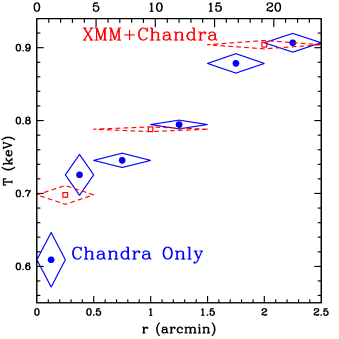
In Table 4 we list the $\chi^{2}$ values for the 1T and 2T (both 3D) fits in shells 1C-6C. In good agreement with the results presented above, we find that the 2T model is a better fit than the 1T model. The temperatures of the 1T and 2T models are plotted in Figure 7 and listed in Table 5. The 1T profile shows excellent agreement with the results obtained from the joint Chandra-XMM fits. In particular, notice that it is the temperature values obtained for shells 2C, 4C, and 6C that agree well with those obtained from the larger shells. The lower temperature values obtained in 1C, 3C, and 5C indicate that the emission-weighted temperatures obtained in shells 1-3 are heavily weighted toward the outer edge of the shell.

The temperatures for the 2T model in the smaller Chandra apertures also agree well with those obtained from the larger apertures. The value of $T_{\rm h}$ in shell 1C is not shown since it has a large best-fitting value and is effectively unconstrained. Note also that results for a small number of error simulations where the normalization of $T_{\rm h}$ in shells 2C and 3C is very small are not included in the error bars indicated in the figure.

It is clear that the 2T models fitted to the Chandra data alone indicate a range of temperatures at a given radius consistent with the 2T models fitted within wider shells. In shells 4C-6C the temperature is consistent with a constant value, $T_{\rm h}$ between 1.3-1.5 keV. The temperature difference within each shell is significantly larger than indicated by the radially varying single-phase model. For example, in shell 5C where the ratio the emission measures for the cool and hot components is 2.3 (best fit), we have $\hbox{{$T_{\rm h}$}}-\hbox{{$T_{\rm c}$}}=0.65\pm 0.13$ keV which is substantially larger ($5\sigma$) than the $\approx 0.03$ keV spread in that shell expected from the single-phase hypothesis.

Perhaps a clearer, more quantitative, indication of the temperature range within the shells is indicated by the GDEM model. The $\chi^{2}$ values and temperature parameters are listed in Tables 4 and 5 are for the GDEM model. Similar to the results obtained from the joint XMM–Chandrafits in larger regions (§4.2.3), the $\chi^{2}$ values obtained for the GDEM model are generally intermediate between the 1T and 2T models, though are clearly better than 1T in all shells except 1C. The parameter values for the GDEM model obtained from the Chandra data alone are consistent with those obtained in the wider apertures (cf. Table 3) though with larger error bars.

As we did in §4.2.3 we can use the GDEM model to test the hypothesis that the temperature profile of the hot gas represents a radially varying single-phase medium. Using the 1T results for shells 3C-6C we would expect the following range of temperatures within shells 4C-6C: $\approx 0.03$ keV within 4C and 5C, and $\approx 0.02$ keV within 6C. Since the 95% confidence lower limit on $\sigma_{T}$ is $\approx 0.10$ in these bins (Table 5), the $1\hbox{{$\sigma_{T}$}}$ temperature range implied by the GDEM model within each shell 4C-6C is at least 0.20 keV – very much larger than than the 0.02-0.03 keV ranges expected from the single-phase hypothesis. (Consistent evidence for multiphase gas is indicated in shells 2C and 3C, but the significance is only at the 2-3 $\sigma$ level.)

We conclude that the improvement in the fits provided by the GDEM and 2T models, as well as the large implied temperature widths obtained for the Chandra data in the thinner shells, provides important additional evidence that a single-phase description of the hot gas in NGC 5044 is inadequate in the central regions.

5 Non-Radial Analysis

5.1 XMM

We performed a two-dimensional spectral analysis to determine whether the multiple components inferred from the analysis assuming spherical symmetry arise from azimuthal temperature fluctuations within each annulus. We searched for azimuthal variations in the temperature and metal abundances using the following simple procedure; results obtained for the abundances are discussed in Paper 2. Within the central CCD of the MOS images we defined a 5x5 array of equally spaced circular extraction regions of $1\arcmin$ radius. Just outside of the central CCD, we defined 12 equally spaced circular regions of $2\arcmin$ radius that surrounded the central CCD. Similar to the azimuthally averaged analysis, to each region we fitted 1T and 2T models modified by foreground Galactic absorption. Each model was fitted simultaneously to the MOS1 and MOS2 data projected on the sky; i.e., no deprojection.

Overall, we find results consistent with the spherically symmetric analysis. The temperatures obtained from the 1T model generally vary significantly only with distance from the center of the image. However, we notice a small asymmetry in the temperature distribution at a radius between $2\arcmin-3\arcmin$. At this radius we find $T\approx 0.9$ keV for $\theta=90\arcdeg-180\arcdeg$ while $T\approx 1.1$ keV elsewhere at this radius ($\theta$ is measured N-E.). This small azimuthal variation cannot account for the wide temperature distributions inferred from the 2T and continuous DEM models.

In fact, when 2T models are fitted to the data, results in very good agreement with those obtained from the spherical analysis are obtained. The fits are improved over the 1T models and values for $T_{\rm c}$ and $T_{\rm h}$ are obtained consistent with those presented for the 2T (2D) models in §4.2.2.

5.2 Chandra

Table 6: Parameters from the Non-Radial Analysis of the Chandra Data

	1T		2T
		$T$		$T_{\rm c}$	$T_{\rm h}$	nc/nh
Region	$\chi^{2}$/dof	(keV)	$\chi^{2}$/dof	(keV)	(keV)	(ratio)
Annulus 2
1A	115.6/79	$0.82\pm 0.005$	81.7/77	$0.80\pm 0.009$	$1.84\pm 0.22$	$3.0\pm 0.6$
1B	58.3/46	$0.76\pm 0.009$	53.8/44	$0.76\pm 0.022$	$\cdots$	$\cdots$
2	114.3/83	$0.78\pm 0.005$	71.8/81	$0.74\pm 0.015$	$1.42\pm 0.13$	$3.0\pm 0.7$
3A	118.0/82	$0.81\pm 0.005$	79.6/80	$0.78\pm 0.010$	$1.52\pm 0.19$	$3.3\pm 0.8$
3B	42.5/42	$0.82\pm 0.010$	35.0/40	$0.82\pm 0.015$	$\cdots$	$\cdots$
Annulus 3
4	47.6/41	$1.07\pm 0.018$	45.9/39	$1.06\pm 0.059$	$\cdots$	$\cdots$
5	65.3/40	$1.12\pm 0.031$	55.8/38	$1.04\pm 0.067$	$\cdots$	$\cdots$
6A	80.4/61	$0.77\pm 0.013$	54.8/59	$0.73\pm 0.017$	$1.56\pm 0.21$	$2.9\pm 0.8$
6B	33.1/31	$0.75\pm 0.017$	26.6/29	$0.67\pm 0.038$	$1.14\pm 0.19$	$2.1\pm 1.1$

Figure 8: Portion of the archival Chandra ACIS-S image located at the center of NGC 5044 adaptively smoothed using the CIAO task CSMOOTH. Heavy circles mark the limits of annuli 2 and 3. Overlaid are several regions used in our non-radial analysis (see §5.2). Region labels match Table 6.

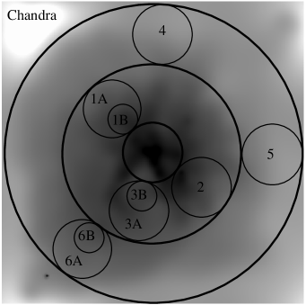
We have performed a similar but independent two-dimensional analysis on the Chandra data. The higher spatial resolution of Chandra allows a more definitive test of the existence of large-scale multiple temperature gas components, by allowing regions as small as a few arcseconds in radius to be analyzed in principle. To directly compare with the azimuthally-averaged analysis, we have chosen circular regions which fall within annuli 2 and 3 defined in Table 1. In Fig. 8 we present several representative regions from this analysis overlaid on a smoothed Chandra image (we note that we have analyzed similar regions across the entire image, but do not find further variation beyond what we report below). Six of these representative regions are 30″ in radius, thus reaching the edge of the annulus they fall within. In addition, we have chosen three smaller regions 15″ in radius which lie within the larger regions, and would fall within the thinner annuli 3C and 5C (defined in Table 4). Some of the regions were placed intentionally in the areas of bright or faint emission visible in the smoothed image, which might be expected to exhibit the strongest spectral variations. As above, in each region we fitted 1T and 2T models modified by foreground Galactic absorption.

In Table 6 we present the results of the 1T and 2T fits for the selected regions shown in Fig. 8. We again find results entirely consistent with the spherically symmetric analysis. For the 1T model, the temperatures from regions lying within annulus 2 are clearly grouped about the value obtained for the entire annulus (cf. Figure 3), not deviating enough to explain the multi-temperature results of the annular analysis. In annulus 3, we see the same asymmetry as observed in the XMM non-radial analysis, with $T\approx 0.8$ keV for $\theta=90\arcdeg-180\arcdeg$ while $T\approx 1.1$ keV elsewhere at this radius. Again, this variation cannot account for the wide temperature distributions inferred from the 2T and continuous DEM models.

The 2T model fits provide an impressive confirmation of this result. For regions 1A, 2, 3A, 6A, and 6B, the 2T models are significantly improved over the 1T models, and obtain values for $T_{\rm c}$ and $T_{\rm h}$ consistent with those fit to the entire annulus (§4.2.2). The strongest constraints are within annulus 3, which is expected since the emission measures of the hotter and cooler components are most similar there (§4.2.2; see Figure 4). For the four remaining regions, there is insufficient S/N to constrain the value of a second temperature component. In these regions (1B, 3B, 4, 5), a second temperature component of similar temperature and relative emission measure strength as found in other regions can be added without significant effect on the fit. We emphasize that regions 1B and 3B are simply subsets of their surrounding regions 1A and 3A, wherein a 2T model improved the fit. Presumably, in a longer exposure of the smaller regions, the same 2T result would obtain; i.e., while present, the 2T model is simply unconstrained in the low S/N regime.

Spatial variations in temperature could also be investigated with a hardness ratio map, an analysis which has been performed by Tamura et al. (2003). They do not find any significant azimuthal hardness variations, consistent with our non-radial analysis here.

6 Systematic Errors

This section contains a detailed investigation of systematic errors on the temperature measurements. Those readers who are not interested in these technical details can safely skip ahead to §7.

6.1 Calibration

6.1.1 XMM–EPIC vs. Chandra–ACIS

Table 7: Comparison of Temperatures from XMM and Chandra

	1T			2T
	$T$			$T_{\rm c}$			$T_{\rm h}$
Annulus	XMM	Chandra	%	XMM	Chandra	%	XMM	Chandra	%
1	$0.764\pm 0.005$	$0.738\pm 0.009$	$3\pm 1$	$0.747\pm 0.006$	$0.724\pm 0.010$	$3\pm 2$	$1.62\pm 0.11$	$2.08\pm 0.31$	$-28\pm 20$
2	$0.814\pm 0.004$	$0.794\pm 0.004$	$3\pm 1$	$0.790\pm 0.002$	$0.782\pm 0.005$	$1\pm 1$	$1.46\pm 0.04$	$1.54\pm 0.07$	$-5\pm 6$
3	$0.990\pm 0.004$	$0.975\pm 0.005$	$2\pm 1$	$0.830\pm 0.005$	$0.835\pm 0.008$	$-1\pm 1$	$1.36\pm 0.03$	$1.41\pm 0.06$	$-4\pm 5$

We have examined possible systematic errors in the measurements of the temperatures arising from calibration differences between the XMM and Chandra CCDs. In Table 7 we list the temperatures obtained from 1T (2D) and 2T (2D) models fitted separately to the XMM and Chandra data; i.e., the MOS and pn data were fitted simultaneously while the Chandra data were fitted alone. We focus on 2D models so that the fits for a specific annulus are independent of results obtained from fits to adjacent regions at larger radii.

Using the 1T model the XMM and Chandra data in annuli 1 and 3 give values of $Z_{\rm Fe}$ that agree within 3% and are consistent within their $3\sigma$ statistical errors. The temperatures of the 2T model are more uncertain, and the XMM and Chandra temperatures are consistent within their $1-1.5\sigma$ errors.

6.1.2 EPIC and ACIS CCDs vs. RGS Gratings

We have compared results obtained from our analysis of NGC 5044 using the XMM and Chandra CCDs to the published results obtained for the XMM RGS obtained by Tamura et al. (2003). First, by comparing the emission measures obtained within our extraction radii with the published emission measure for the RGS data by Tamura et al. (2003) and a separate analysis of the RGS data (T. Fang 2003, private communication) we conclude that the effective RGS aperture corresponds to a circular aperture with radius $R\approx 30\arcsec-40\arcsec$; i.e., essentially our radius bin 1.

Tamura et al. (2003) find that a 2T (2D) model is a significant improvement over a 1T model. In their analysis they (1) restrict their analysis to 0.44-1.55 keV, (2) only allow the iron and oxygen abundances to vary, (3) use the solar abundance table of Anders & Grevesse (1989), and (4) use a plasma code essentially corresponding to the mekal code (Kaastra & Mewe, 1993; Liedahl et al., 1995) in xspec. They obtain the following parameters for the 2T model: $\hbox{{$T_{\rm c}$}}=0.7$ keV (no error quoted), $\hbox{{$T_{\rm h}$}}=1.07\pm 0.03$ keV, $\hbox{{$Z_{\rm Fe}$}}=0.55\pm 0.05\hbox{{$Z_{\odot}$}}$, and $\hbox{{$Z_{\rm O}$}}/\hbox{{$Z_{\rm Fe}$}}=0.51\pm 0.06$ in solar units. If we follow the same procedures (1)-(4) for the EPIC and ACIS data within radial bin 1 we obtain the following best-fitting values for the 2T model: $\hbox{{$T_{\rm c}$}}=0.68$, $\hbox{{$T_{\rm h}$}}=1.08$ keV, $\hbox{{$Z_{\rm Fe}$}}=0.58\hbox{{$Z_{\odot}$}}$, and $\hbox{{$Z_{\rm O}$}}/\hbox{{$Z_{\rm Fe}$}}=0.46$ in solar units. These results are in excellent agreement with Tamura et al.’s results for the RGS.

We conclude that the RGS and the EPIC and ACIS CCDs give fully consistent results when the same models are fitted over the same energy ranges for each instrument. In particular, the RGS corroborates the improvement of a 2T (2D) model over a 1T (2D) model. However, since they are unable to perform a deprojection analysis, Tamura et al. (2003) could not determine whether the extra temperature component arises only from projection of gas from larger radii. (The consistency of the metal abundances is discussed further in Paper 2.)

6.2 Plasma Codes

We compared the results obtained using the apec code to those obtained using the mekal code (Kaastra & Mewe, 1993; Liedahl et al., 1995) to assess the importance of different implementations of the atomic physics and different emission line lists in the plasma codes. In every case examined we found no qualitative differences between results obtained from each code; e.g., the fitted temperatures usually agree to within $\sim 5\%$. The $\chi^{2}$ values obtained for the multitemperature models are also very similar. Some significant quantitative differences in $\chi^{2}$ values are observed for the 1T models, but there is no qualitative difference in the fits. For example, for shell 3 the 1T (3D) mekal model gives $\chi^{2}=1535.3$ for 693 dof compared to $\chi^{2}=1338.2$ for the apec code. Visual inspection of these fits and residuals reveals no noticeable differences between the two fits except for slightly more pronounced residuals in the Fe L region in the mekal fit.

(We note that we explored the the validity of the assumption of ionization equilibrium using the vnei model in xspec. We found no improvement in the fit for a single-temperature model when allowing for departures from ionization equilibrium.)

6.3 Bandwidth

We explored the sensitivity of our results our default lower limit of the bandpass, $\hbox{{$E_{\rm min}$}}=0.5$ keV. For comparison we performed 1T and 2T fits (both in 3D) with $\hbox{{$E_{\rm min}$}}=0.3$ keV and $\hbox{{$E_{\rm min}$}}=0.7$ keV. The fitted temperatures are generally consistent between models with $E_{\rm min}$ between 0.3-0.7 keV. However, the $\chi^{2}$ values indicate that the improvement of the 2T model over the 1T model decreases significantly as $E_{\rm min}$ increases. In shell 3, for example, we obtain $\chi^{2}$/dof of 1427.9/774 (1T) and 957.5/772 (2T) for $\hbox{{$E_{\rm min}$}}=0.3$ keV , 1189.0/693 (1T) and 836.0/691 (2T) for $\hbox{{$E_{\rm min}$}}=0.5$ keV, 916.4/614 (1T) and 730.5/612 (2T) for $\hbox{{$E_{\rm min}$}}=0.7$ keV (each model is 3D). Similar behavior is observed for shells 1,3, and 4.

This decreasing of the need for multitemperature models with increasing $E_{\rm min}$ demonstrates that the residuals in the Fe L lines near 1 keV for 1T models are not the sole driving force for the 2T and other multitemperature models. This is significant since it implies that remaining inaccuracies in the the Fe L lines in the plasma codes cannot be solely responsible for the improvement of the multitemperature models over 1T models. Conversely, large bandwidth is seen to be imperative in the search for, and constraint of, multitemperature models of the hot gas.

6.4 Variable $N_{\rm H}$

Table 8: 1T and 2T Models with Variable Absorption

	1T		2T
		$\Delta\hbox{{$N_{\rm H}$}}$		$\Delta\hbox{{$N_{\rm H}$}}$
Shell	$\chi^{2}$/dof	($10^{20}$ cm-2)	$\chi^{2}$/dof	($10^{20}$ cm-2)
1	688.7/450	$5.2\pm 0.8$	637.8/448	$1.9\pm 0.9$
2	1059.8/688	$7.0\pm 0.4$	916.7/686	$3.4\pm 0.6$
3	1120.9/692	$4.2\pm 0.4$	828.2/690	$1.9\pm 0.6$
4	616.3/481	$4.0\pm 0.7$	533.6/479	$1.3\pm 0.8$
5	510.3/453	$0.8\pm 0.7$	485.2/451	$0.4\pm 0.8$
6	551.4/468	$0.8\pm 0.8$	513.8/466	$0.4\pm 1.0$
7	561.2/514	$-1.8\pm 0.8$	544.7/512	$-2.4\pm 0.9$
8	674.3/560	$0.5\pm 0.7$	657.9/558	$0.8\pm 1.0$

Since the lever-arm provided by the bandwidth below $\sim 0.7$ keV is an important constraint on the multitemperature models, it should be expected that the fits may also be improved – to some extent – by allowing for intrinsic (continuous) photoelectric absorption from cold gas. In Table 8 we present results for the 1T (3D) and 2T (3D) models where we have allowed $N_{\rm H}$ of the foreground absorber component to be a free parameter. (We have examined a suite of cold absorber models and they give results similar to those for the simple foreground-screen cold absorber model.) In shells 1-2 the 1T model is improved significantly with variable absorption. However, in shells 1-4 the 2T model is still clearly preferred over the 1T model when allowing for variable absorption in each case. In fact, variable $N_{\rm H}$ actually improves the 2T model very little; i.e., the 2T model with Galactic absorption (Table 1) is itself superior to the 1T model with variable $N_{\rm H}$in shells 1-4.

The superior fits provided by the 2T (and other multitemperature models like the PLDEM) with Galactic absorption, and the relatively insignificant improvement to the multitemperature models obtained when intrinsic absorption is allowed for, indicates to us that there is little motivation to consider intrinsic absorption models. Moreover, the variable-$N_{\rm H}$models imply large amounts of absorbing material in shells 1-4; e.g., taking $\Delta\hbox{{$N_{\rm H}$}}=2.5\times 10^{20}$ cm^-2 in shells 1-2 leads to an absorbing mass, $M_{\rm abs}\approx m_{\rm H}\Delta\hbox{{$N_{\rm H}$}}\pi(14\,\rm kpc)^{2}\approx 10^{9}\hbox{{$M_{\sun}$}}$ assuming solar abundances and that the absorber is uniformly distributed; this is a lower limit if the abundances are sub-solar and the absorber is non-uniform. This large absorbing mass is almost as large as that of the hot gas. Yet this amount of cold material, whether it be from optical line emitting gas or dust (e.g., Goudfrooij et al., 1994) or from atomic or molecular gas (e.g., Bregman et al., 1992; O’Dea et al., 1994), has never been seen in NGC 5044 or other “cooling flow” galaxies. (We note that the fitted values of $N_{\rm H}$ for both the 1T and 2T models at large radius are consistent with the Galactic value within their $1-2\sigma$ errors.)

Since the multitemperature models with $\hbox{{$N_{\rm H}$}}=\hbox{{$N_{\rm H}^{\rm Gal}$}}$ provide better fits within the central $\approx 30$ kpc, there is no obvious sharp absorption feature in the spectrum, and there is no evidence from observations in other wavebands for the large quantities of cold absorbing material implied by the fitted values of $N_{\rm H}$, we do not take seriously the results obtained from the intrinsic cold absorber models.

6.5 Background

Since NGC 5044 is sufficiently bright the fitted temperature values are quite insensitive to errors in the background normalization. For example, even if we do not subtract the background in the bounding annulus (where background is most important) the temperature we obtain for a 1T model differs only by 10% from the background-subtracted value. Within the inner shells the background effect is negligible; e.g., in shell 2 if the background is not subtracted we obtain a 1T temperature that differs by $0.2\%$ from the background-subtracted value.

7 Spectral Analysis within a Large Aperture

Figure 9: EPIC MOS1, MOS2, pn and ACIS-S3 spectra accumulated within a circular aperture of radius, $R=2.5\arcmin$ (24 kpc), fitted with (Left panel) a single temperature (1T) model and (Right panel) a two-temperature (2T) model (no deprojection is performed). In each case the apec plasma model is used and the solar abundances are taken from Grevesse & Sauval (1998) which use the new (smaller) photospheric value for the iron abundance. The models are the same as discussed in §4.2.1 and §4.2.2 for the spatially resolved analysis. That is, Galactic absorption is assumed and the following metal abundances are free parameters: O, Ne, Mg, Si, S, Fe and all other abundances are tied to Fe in their solar ratios. For the 2T model the abundances of each temperature component are tied together in the fits.

Table 9: Selected Results for Models Fitted Within a Large Aperture

		$\Delta\hbox{{$N_{\rm H}$}}$	$T_{\rm c}$	$T_{\rm h}$		$T_{\rm min}$	$T_{\rm max}-T_{\rm min}$
Model	$\chi^{2}$/dof	($10^{20}$ cm-2)	(keV)	(keV)	$\alpha$	(keV)	(keV)
1T, Galactic $N_{\rm H}$	4197.4/869	$\cdots$	$0.897\pm 0.002$	$\cdots$	$\cdots$	$\cdots$	$\cdots$
1T, variable $N_{\rm H}$	3879.5/868	$4.5\pm 0.3$	$0.878\pm 0.002$	$\cdots$	$\cdots$	$\cdots$	$\cdots$
2T, Galactic $N_{\rm H}$	1356.8/867	$\cdots$	$0.792\pm 0.002$	$1.41\pm 0.02$	$\cdots$	$\cdots$	$\cdots$
2T, variable $N_{\rm H}$	1313.0/866	$3.0\pm 0.6$	$0.779\pm 0.006$	$1.28\pm 0.04$	$\cdots$	$\cdots$	$\cdots$
PLDEM, Galactic $N_{\rm H}$	1373.0/867	$\cdots$	$\cdots$	$\cdots$	$-3.0\pm 0.1$	$0.681\pm 0.005$	$1.5\pm 0.1$

Table 10: Fits to Simulated Data of Radially Varying Models Within a Large Aperture

	$\chi^{2}$/dof
Model	Sim #1	Sim #2	Sim #3
1T, Galactic $N_{\rm H}$	1809.8/839	2469.2/855	3731.6/861
1T, variable $N_{\rm H}$	1805.3/838	1309.1/854	3611.3/860
2T, Galactic $N_{\rm H}$	865.6/837	1105.4/853	980.0/859

Thus far we have fitted models to the XMM and Chandra spectra of a particular radial bin independently of the spectra in other radial bins. (Although a deprojected model for a specific radial bin does account for the projected emission from exterior shells, the spectral fitting is not performed simultaneously with other shells.) Here we consider models fitted to the total XMM and Chandra spectral data accumulated within radial bins 1-3; i.e., within a circular aperture of radius, $R=2.5\arcmin$ (24 kpc). We focus on this central region where there is both Chandra and XMM data and evidence for multiphase gas. Our objective is to show that the preference for the multiphase models indicated by the fits to the individual radial bins 1-3 is rendered even more significant when the data in these bins are analyzed simultaneously in a single aperture.

First we summarize the results (Table 9) of fitting 1T, 2T, and PLDEM models (all 2D for this exercise) to the spectral data within $R=2.5\arcmin$. As expected, the 1T model is an even worse fit than within the individual radial bins 1-3. The best-fitting 1T model shown in Figure 9 displays more pronounced residuals near 1 keV (i.e., characteristic of the “Fe Bias”) than observed for the fit only to radial bin 2 shown in Figure 5. The Chandra ACIS-S3 data have the most pronounced $\chi^{2}$ residuals in Figure 9 near 1 keV, but we note that the fractional residuals between the model and data are very similar for both the EPIC and ACIS CCDs. Allowing for variable $N_{\rm H}$ does not improve the 1T fits significantly, despite the fact that a large excess value for the column density is indicated.

However, the addition of a second temperature component (i.e., 2T model) provides a vastly improved fit with small residuals near 1 keV similar to the residuals at other energies (Figure 9). The PLDEM model fits nearly as well as the 2T model, and the quality of both of these fits is about as good as could be hoped for considering the simplicity of these models and that we know the spectral properties do vary with radius within the $R=2.5\arcmin$ aperture. (Allowing for variable $N_{\rm H}$ also provides negligible improvement for the multitemperature models even though a large fitted value of excess $N_{\rm H}$ is indicated – the 2T result is shown in Table 9.)

Now we wish to compare these results to those that should have been obtained if the real data were actually described by the radially varying 1T and 2T models in shells 1-3 obtained in §4.2.1 and §4.2.2. To perform this comparison we follow the general approach discussed in §5.3 of Buote (1999). We take the 1T (3D) models in shells 1-3 obtained from the real EPIC and ACIS data (§4.2.1) and simulate EPIC and ACIS spectra appropriate for the NGC 5044 observations using the fakeit routine in xspec. These simulated spectra also contain the projected emission from external shells obtained from our deprojection analysis. The resulting simulated source and background pha files for radial bins 1-3 are then summed (separately for each detector) and analyzed in the same way as done in Table 9. We refer to this simulated radially varying 1T model within $R=2.5\arcmin$ as “Sim #1” in Table 10. “Sim #2” and “Sim #3” in Table 10 are prepared in the same way as “Sim #1” except they refer respectively to the 1T (3D) model with variable $N_{\rm H}$ (§6.4) and 2T (3D) model with Galactic $N_{\rm H}$ (§4.2.2).

Fits to Sim #1 using 1T models give $\chi^{2}\approx 1800$ which are much smaller than the values of $\chi^{2}\approx 4000$ obtained for the real data in Table 9. The 2T model is also a somewhat better fit than for the real data and provides a formally acceptable fit. Although similar to the real data the 2T fit is superior to the 1T fit, and there is negligible improvement when allowing for variable absorption, the much smaller values of $\chi^{2}$ for the 1T models fitted to Sim #1 rule out the radially varying 1T models with Galactic absorption.

Qualitatively different results are obtained for fits to Sim #2. Similar to Sim #1 the fitting the 1T model with Galactic $N_{\rm H}$has yields a much lower value of $\chi^{2}$ than obtained for the real data. However, the 1T model with variable $N_{\rm H}$ provides a very large improvement in the fit – almost as good as the 2T model with Galactic $N_{\rm H}$. This behavior is totally inconsistent with the results obtained from the real data in Table 9, and we conclude that the radially varying 1T model with variable $N_{\rm H}$ is not a viable description of the spectral data within $R=2.5\arcmin$.

In contrast, the $\chi^{2}$ values obtained for fits to Sim #3 are very similar to those obtained for the real data in Table 9. Since only fits to Sim #3 can reproduce the results of fitting the real data, this is strong evidence that the multitemperature models (in this case the radially varying 2T model, but this also applies to the PLDEM model) are required within the central $R=2.5\arcmin$ (24 kpc) of NGC 5044.

8 Discussion: Two-Phase Model

Figure 10: Volume filling factor of the cooler component required to maintain pressure equilibrium between the cooler and hotter phases in the 2T (3D) model obtained from simultaneous fitting of the XMM and Chandra data. Due to the expected contribution of emission from discrete sources, the value in the central bin is quite uncertain and is consistent with unity. The units are arcminutes on the bottom axis and kpc on the top axis.

Our spectral deprojection analysis of the XMM and Chandra data of NGC 5044 indicates that a single-phase description of the hot gas is inadequate for $r\lesssim 30$ kpc. Of the simple multiphase models we considered, the 2T and PLDEM models provide the best fits in the central regions. Each of these models describes a limited multiphase plasma where the cooler temperature components ($\sim 0.7$ keV) dominate for $r\lesssim 10$ kpc, the contributions of cooler and hotter ($\sim 1.4$ keV) components are similar for $r\approx 20-30$ kpc, while at larger radii the hotter components dominate so that the gas is consistent with a single-phase medium.

These results for the 2T model are very similar to those obtained from an analysis of the XMM data of the group NGC 1399 (Buote, 2002). The temperature of the extended hotter component, $\hbox{{$T_{\rm h}$}}\sim 1.4$ keV, is consistent with the virial temperature of a surrounding group of mass $\approx 10^{13}\hbox{{$M_{\sun}$}}$, whereas the temperature of the centrally concentrated cooler component, $\hbox{{$T_{\rm c}$}}\sim 0.7$ keV, is similar to the kinetic temperature of the stars. These parameters suggest a physical association of the hotter component with the ambient group gas and the cooler component with stellar ejecta from the dominant central galaxy.

A potential problem with this scenario is that it might be expected that these phases should mix very rapidly for a system in equilibrium. However, the sharp edge in the surface brightness and isophote center offset for $R\approx 5\arcmin-6\arcmin$ discussed in §3 are suggestive of a “cold front” such as has been observed in several clusters with Chandra (e.g. Markevitch et al., 2002). The surface brightness edge in the MOS image of NGC 5044 near $R\approx 50$ kpc to the NW essentially divides the regions where the cooler and hotter gas phases are most prominent.

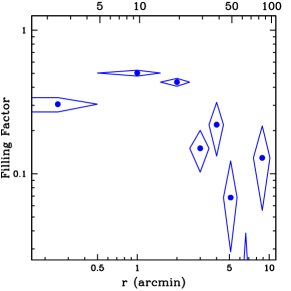
Although the cold front can explain the radial transition from cooler to hotter dominance, the phases clearly co-exist over a large range in radius. For this to occur we expect the phases to be in pressure equilibrium. We have calculated the volume filling factor ($f_{\rm c}$) of the cooler component of the 2T model required to maintain pressure equilibrium between the two phases. The result is plotted in Figure 10.

For $r\gtrsim 30$ kpc we have $f_{\rm c}\sim 0.1$ indicating that the cooler gas occupies only a small fraction of the shell volume. In contrast, for shells 2-3 ($r\sim 5-25$ kpc) we have $f_{\rm c}\approx 0.5$ meaning that each phase occupies half the volume. In shell 1 ($r\lesssim 5$ kpc) the value shown ($f_{\rm c}\approx 0.3$) is actually a lower limit because the value of $T_{\rm h}$ is overestimated due to contamination from discrete sources (§4.2.2).

9 Conclusions

The spectral deprojection analysis of XMM and Chandra data favors a two-phase (2T) or limited multi-phase medium (PLDEM) within the central $r\sim 30$ kpc of NGC 5044. The cooler component in the 2T models has a temperature $\hbox{{$T_{\rm c}$}}\sim 0.7$ keV similar to the kinetic temperature of the stars in the central galaxy NGC 5044, and the hotter component has a temperature $\hbox{{$T_{\rm h}$}}\sim 1.4$ keV characteristic of the massive $\sim 10^{13}$ $M_{\odot}$ dark halo of the surrounding galaxy group. Nevertheless, both temperature components appear at every radius $\lesssim 30$ kpc. In spite of the similarity of the hot phase temperature $T_{\rm h}$ and the group virial temperature at all radii, it is likely that gas at small radii with temperature $T_{\rm h}$ is heated by a central AGN. Some additional heating at large radii could arise from the energy associated with establishing the cold front near $r\sim 30$ kpc, as suggested by the sharp edge visible in the EPIC MOS and pn images.

The need for two discrete temperatures in the 2T models cannot be attributed solely to the Fe-L lines at $\sim 1$ keV, which still may be uncertain in the plasma codes, but is also required by the spectrum below 0.7 keV. Our comparison of results using the apec and mekal codes in §6.2 indicates that even large differences in the plasma codes have a small effect at the moderate resolution of the EPIC and ACIS CCDs.

As an alternative, and possibly more physically plausible model, we have shown that a continuous, but limited, range of temperatures in each spherical shell (PLDEM) can explain the NGC 5044 data for $r\lesssim 30$ kpc as well as the 2T model. However, the range of temperatures required in each spherical shell exceeds the radial temperature variation of the best-fitting single-phase models across the same shell. For either type of thermal model there is no evidence at any radius for gas at temperatures $\lesssim 0.7$ keV. These results are very similar to our previous 2T models of NGC 5044 using ASCA data (Buote, 1999). However, within $r\sim 30$ kpc the ASCA data lacked the spatial resolution of XMM and Chandra and could not distinguish between a single-phase medium in which the gas temperature varies with radius, a two-phase (2T) medium, or multi-phase gas at every radius.

The remarkable irregularities visible for $r\lesssim 10$ kpc in the Chandra image of NGC 5044 (Figure 1) support the notion of fluctuations in the gas density and, by implication, also in the gas temperature. In pressure equilibrium the ratio of X-ray emissivities in the two phases should be approximately, $[(n_{\rm e})_{\rm c}/(n_{\rm e})_{\rm h}]^{2}\propto(\hbox{{$T_{\rm h}$}}/\hbox{{$T_{\rm c}$}})^{2}\approx 5$, which may be sufficient to account for the conspicuous surface brightness fluctuations in Figure 1. Within the central annulus ($R=0.5\arcmin\approx 5$ kpc), which includes nearly half the optical image of the NGC 5044 galaxy, the X-ray spectrum is further complicated by hard $\sim 10$ keV bremsstrahlung radiation from X-ray binary stars, so the precise range of gas temperatures is less accurately determined in this region.

The 2T or limited multi-phase thermal properties of NGC 5044 are very similar to those of the bright galaxy group NGC 1399 revealed by XMM (Buote, 2002). A 2T model is also preferred by Molendi (2002) in his XMM analysis of M87. However, Molendi argues that the temperature range $\hbox{{$T_{\rm h}$}}-\hbox{{$T_{\rm c}$}}$ implied for each annulus by his 2T model for M87 is consistent with a radially varying single-phase temperature except in regions where the X-ray image is clearly distorted by interaction with the central radio source. Nevertheless, the pattern that is emerging from observations of NGC 5044 and NGC 1399 may differ substantially from the gasdynamical models of groups and clusters constructed by Brighenti & Mathews (1999, 2002). In the gasdynamical models relatively cool ejecta from stellar mass loss mix thermally on small scales with hotter ambient group or cluster gas to reproduce the single-phase radial temperature profiles typically observed in groups and clusters. Instead, our observations suggest a limited range of thermal phases that are incompletely mixed at every radius, which, if viewed as a single-phase gas, can reproduce the same typical “cooling flow” thermal profile but with a reduction in the quality of the spectral fit.

References

- Anders & Grevesse (1989) Anders, E. & Grevesse, N. 1989, Geochim. Cosmochim. Acta, 53, 197
- Arnaud (1996) Arnaud, K. A. 1996, in ASP Conf. Ser. 101: Astronomical Data Analysis Software and Systems V, Vol. 5, 17
- Bregman et al. (1992) Bregman, J. N., Hogg, D. E., & Roberts, M. S. 1992, ApJ, 387, 484
- Brighenti & Mathews (1999) Brighenti, F. & Mathews, W. G. 1999, ApJ, 512, 65
- Brighenti & Mathews (2002) —. 2002, ApJ, 567, 130
- Buote (1999) Buote, D. A. 1999, MNRAS, 309, 685
- Buote (2000a) —. 2000a, ApJ, 539, 172
- Buote (2000b) —. 2000b, MNRAS, 311, 176
- Buote (2002) —. 2002, ApJ, 574, L135
- Buote & Fabian (1998) Buote, D. A. & Fabian, A. C. 1998, MNRAS, 296, 977
- Buote et al. (2003a) Buote, D. A., Lewis, A. D., Brighenti, F., & Mathews, W. G. 2003a, in preparation
- Buote et al. (2003b) —. 2003b, ApJ, submitted (astro-ph/0303054)
- Churazov et al. (2001) Churazov, E., Brüggen, M., Kaiser, C. R., Böhringer, H., & Forman, W. 2001, ApJ, 554, 261
- Condon et al. (1998) Condon, J. J., Cotton, W. D., Greisen, E. W., Yin, Q. F., Perley, R. A., Taylor, G. B., & Broderick, J. J. 1998, AJ, 115, 1693
- Craig & Brown (1976) Craig, I. J. D. & Brown, J. C. 1976, A&A, 49, 239
- David et al. (1995) David, L. P., Jones, C., & Forman, W. 1995, ApJ, 445, 578
- David et al. (1994) David, L. P., Jones, C., Forman, W., & Daines, S. 1994, ApJ, 428, 544
- David et al. (2001) David, L. P., Nulsen, P. E. J., McNamara, B. R., Forman, W., Jones, C., Ponman, T., Robertson, B., & Wise, M. 2001, ApJ, 557, 546
- Fabian et al. (2000) Fabian, A. C., Sanders, J. S., Ettori, S., Taylor, G. B., Allen, S. W., Crawford, C. S., Iwasawa, K., Johnstone, R. M., & Ogle, P. M. 2000, MNRAS, 318, L65
- Goudfrooij et al. (1994) Goudfrooij, P., Hansen, L., Jorgensen, H. E., & Norgaard-Nielsen, H. U. 1994, A&AS, 105, 341
- Grevesse & Sauval (1998) Grevesse, N. & Sauval, A. J. 1998, Space Science Reviews, 85, 161
- Johnstone et al. (1992) Johnstone, R. M., Fabian, A. C., Edge, A. C., & Thomas, P. A. 1992, MNRAS, 255, 431
- Kaastra & Mewe (1993) Kaastra, J. S. & Mewe, R. 1993, A&AS, 97, 443
- Liedahl et al. (1995) Liedahl, D. A., Osterheld, A. L., & Goldstein, W. H. 1995, ApJ, 438, L115
- Markevitch et al. (2002) Markevitch, M., Vikhlinin, A., & Forman, W. R. 2002, in Matter and Energy in Clusters of Galaxies, eds. S. Bowyer and C.-Y. Hwang, ASP Conf. Ser., vol X, in press (astro-ph/0208208)
- McNamara et al. (2000) McNamara, B. R., Wise, M., Nulsen, P. E. J., David, L. P., Sarazin, C. L., Bautz, M., Markevitch, M., Vikhlinin, A., Forman, W. R., Jones, C., & Harris, D. E. 2000, ApJ, 534, L135
- McWilliam (1997) McWilliam, A. 1997, ARA&A, 35, 503
- Molendi (2002) Molendi, S. 2002, ApJ, 580, 815
- O’Dea et al. (1994) O’Dea, C. P., Baum, S. A., Maloney, P. R., Tacconi, L. J., & Sparks, W. B. 1994, ApJ, 422, 467
- O’Sullivan et al. (2001) O’Sullivan, E., Forbes, D. A., & Ponman, T. J. 2001, MNRAS, 328, 461
- Tamura et al. (2003) Tamura, T., Kaastra, J. S., Makishima, K., & Takahashi, I. 2003, A&A, 399, 497
- Tonry et al. (2001) Tonry, J. L., Dressler, A., Blakeslee, J. P., Ajhar, E. A., Fletcher, A. ., Luppino, G. A., Metzger, M. R., & Moore, C. B. 2001, ApJ, 546, 681
- Townsley et al. (2002) Townsley, L. K., Broos, P. S., Nousek, J. A., & Garmire, G. P. 2002, nuclear Instruments and Methods in Physics Research, in press (astro-ph/0111031)