The Dwarf Spheroidal Companions to M31: Variable Stars in Andromeda VI

Abstract

We have surveyed Andromeda VI, a dwarf spheroidal galaxy companion to M31, for variable stars using F450W and F555W observations obtained with the Hubble Space Telescope. A total of 118 variables were found, with 111 being RR Lyrae, 6 anomalous Cepheids, and 1 variable we were unable to classify. We find that the Andromeda VI anomalous Cepheids have properties consistent with those of anomalous Cepheids in other dwarf spheroidal galaxies. We revise the existing period–luminosity relations for these variables. Further, using these and other available data, we show that there is no clear difference between fundamental and first-overtone anomalous Cepheids in a period-amplitude diagram at shorter periods, unlike the RR Lyrae. For the Andromeda VI RR Lyrae, we find that they lie close to the Oosterhoff type I Galactic globular clusters in the period-amplitude diagram, although the mean period of the RRab stars, $\langle P_{ab}\rangle=0.588$d, is slightly longer than the typical Oosterhoff type I cluster. The mean $V$ magnitude of the RR Lyrae in Andromeda VI is $25.29\pm 0.03$, resulting in a distance $815\pm 25$ kpc on the Lee, Demarque, & Zinn distance scale. This is consistent with the distance derived from the $I$ magnitude of the tip of the red giant branch. Similarly, the properties of the RR Lyrae indicate a mean abundance for Andromeda VI which is consistent with that derived from the mean red giant branch color.

1 Introduction

Galactic dwarf spheroidal galaxies (dSphs) have been shown to be quite diverse in their star formation histories (e.g., Da Costa 1998; Grebel 1999). These galaxies generally also possess a range in metallicity among their stars. A detailed examination of these and other dwarf galaxies is important in understanding galaxy formation and gives insight into cosmology (e.g., Klypin et al. 1999). The diverse stellar populations in these systems is also reflected in their variable stars. dSphs contain significant numbers of RR Lyrae (RRL) implying an older ($t>10$ Gyr) stellar population. Contrary to Galactic globular clusters whose RRab stars can be classified into one of two Oosterhoff types (Oosterhoff 1939), the mean period of the RRab stars in a number of dSphs is “intermediate” between the two types. A second difference between Galactic globular clusters and dSphs as regards their variable star content, is the existence of anomalous Cepheids (ACs) in dSphs. Only one AC is known among the entire Galactic globular cluster population, V19 in NGC 5466 (Zinn & King 1982), but there exists at least one AC in every dSph surveyed for variable stars. These fundamental differences between dSphs and Galactic globular clusters are presumably indicative of the differences in the stellar populations of these systems.

Clearly, a large and diverse sample of variable stars in dSphs can contribute to the understanding of the underlying stellar populations in these systems. While there have been many detailed variability surveys for the Galactic dSphs (e.g., Kaluzny et al. 1995; Mateo, Fischer, & Krzeminski 1995; Siegel & Majewski 2000; Held et al. 2001; Bersier & Wood 2002), there are none available for the M31 dSph companions. In this paper we examine the variable star content of the M31 dSph Andromeda VI (And VI, also known as the Pegasus dSph). Armandroff, Jacoby, & Davies (1999, hereafter AJD99) found And VI to have a mean metallicity of $\langle{\rm[Fe/H]}\rangle=-1.58\pm 0.20$ dex from the mean ($V$–$I$) color of the red giant branch. This places And VI among the more metal–rich of the dSphs within the Local Group. AJD99 also derived a distance of $775\pm 35$ kpc for And VI from the $I$ magnitude of the tip of the red giant branch. A detailed analysis of the And VI color–magnitude diagram, based on HST/WFPC2 images, will be presented in Armandroff et al. (2002). Here, we present the discovery of 118 variables in And VI from that data; 111 RRL, 6 ACs, and 1 whose classification is uncertain. Light curves and mean properties are given for each variable. We then use these data to compare the properties of the And VI variables with those for other dSphs.

2 Observations and Reductions

As part of our GO program 8272, the Hubble Space Telescope imaged And VI with the WFPC2 instrument on 1999 October 25 and, with the same orientation, on 1999 October 27. For each set of observations, four 1100s exposures through the F555W filter and eight 1300s exposures through the F450W filter were taken. The second set of observations was offset slightly from the first set in order to aid in distinguishing real stars from image defects. The images were taken with a gain of 7 electrons/ADU. The raw frames were processed by the standard STScI pipeline. Each frame was separated into individual images for each CCD and the vignetted areas were trimmed using the limits defined in the WFPC2 Handbook.

2.1 Photometry

In order to create a star list for photometry that is relatively free of contamination by cosmic ray events, star detection was performed on a cleaned image. To do this, we used the Peter Stetson routine, montage ii. This program creates a median image from all available images. The advantage of this is that the median image eliminates nearly all of the cosmic rays and other defects that are found on the individual images. A search for stellar objects was then performed on the median image for each CCD using a full-width at half maximum of 1.6 pixels. Aperture photometry on these median images was then obtained using Stetson’s (1992) stand-alone version of daophot ii. An aperture radius of 2.0 pixels was used. The allstar routine was then employed to obtain profile–fitting photometry for the stars on the median images, adopting a fitting radius of 1.6 pixels. The point-spread functions for each CCD were obtained from Peter Stetson; they were created for reducing data in the Extragalactic Distance Scale Key Project (Stetson et al. 1998). The objects that were fit by allstar on the median image were assumed to be stars and not image defects or resolved galaxies.

The master list of objects was then used by allframe (Stetson 1994) to obtain profile-fitting photometry for each individual CCD exposure. This program is designed to reduce all of the images simultaneously for each CCD. The resulting photometry was investigated for variable stars using the Stetson routine daomaster. daomaster compared the rms scatter in the photometric values to that expected from the photometric errors returned by the allframe program. The PC was searched for variable stars and only turned up a handful of candidate RRL with no ACs. Since this small number of RRL would add little to the final results, we decided to ignore the PC data.

2.2 CTE and Aperture Corrections

It is well known that the WFPC2 CCDs suffer from poor charge-transfer efficiency (CTE) which affects the photometry (Holtzman et al. 1995; Stetson 1998; Whitmore, Heyer, & Casertano 1999; Dolphin 2000). In order to correct for this effect we applied equations (2c) and (3c) from Whitmore, Heyer, & Casertano (1999) to the profile-fitting photometry for each frame.

To place the photometry on the system of Holtzman et al. (1995), aperture corrections are required to convert the profile–fit magnitudes to magnitudes within a 5 pixel radius aperture. As part of this process, a comparison of the profile–fit photometry for each individual frame to that for an adopted “reference” frame (the first image in the sequence for the first pointing) was carried out. This revealed that there were cyclic differences from frame–to–frame that followed the exposure sequence of the observations. As a result, we decided to determine the aperture correction for the adopted “reference” frame and base the aperture corrections for the other frames on the differences seen between the profile-fitting photometry of each frame as compared to the “reference” frame.

In order to do this, the difference between the 5 pixel radius aperture magnitudes from the “gcombined” frames for each CCD (Armandroff et al. 2002) and the profile–fit magnitudes for the “reference” frame was then computed for those stars that had no neighbors within a 7 pixel radius. We then generated the weighted mean of these differences for all stars brighter than the horizontal branch by approximately 1 magnitude for each filter. In this calculation, stars whose differences were greater than 0.4 mag were excluded. This gave us the aperture correction for the “reference” frame. The aperture corrections for the rest of the frames were then calculated from the aperture correction for the “reference” frame and the differences in the profile–fit photometry between this frame and each individual frame.

The resulting aperture corrections were then applied to the profile–fit photometry along with the CTE corrections. After correction, the resulting mean differences in the photometry between the frames were, for the most part, below 0.01 mag with the maximum difference being around 0.015 mag.

Figure 1: And VI color-magnitude diagram showing the location of the RR Lyrae and anomalous Cepheids marked as crosses.

3 Light Curves

With at most 16 epochs in F450W and 8 epochs in F555W, phasing the photometry and finding accurate periods in both colors presents a challenge. In order to employ the maximum number of photometric measures in the period finding, we sought to use the F450W and F555W data together. Therefore, we need to determine the magnitude offset for each star to place the F555W observations on the F450W magnitude scale. We began this process by noting that the last F555W observation and the first F450W observation were taken consecutively. Therefore, we can assume that this F555W magnitude, which we denote by $m_{0{\rm,F555W}}$, corresponds to the F450W magnitude, which we denote by $m_{0,{\rm F450W}}$. The other F555W magnitudes are then converted to their F450W equivalents by using the equation:

$$m_{{\rm n,F450W}}=m_{{\rm 0,F450W}}+1.3(m_{{\rm F555W}}-m_{{\rm 0,F555W}})$$ (1)

where $m_{{\rm n,F450W}}$ is the F450W magnitude derived from the F555W magnitude $m_{{\rm F555W}}$. The 1.3 value is the approximate ratio of the amplitudes in $B$ to $V$ for the light curves. This value was determined from a number of RRL in various Galactic GCs which had clean light curves in both colors. While this ratio may not be exactly the same as the F450W to F555W ratio for the amplitudes, a difference of $\pm 0.1$ in the amplitude ratio does not affect the results. This combined dataset was then used to determine the period of the star through the use of routines created by Andrew Layden (Layden & Sarajedini 2000 and references therein). The program is designed to determine the most likely period from the chi–squared minima by fitting the photometry of the variable star with 10 templates over a selected range of periods. Since there is little difference in light curve shape between RRL and ACs, we are confident that the templates will work well for any ACs we find. Due to the aliasing from the observations, these periods were tested in a period–amplitude diagram to determine their accuracy. A small number of RRL with periods scattered from where the majority were found in this diagram were revised in order to reduce the scatter. These typically were stars that had large gaps in their light curves making it difficult to accurately determine their period. The combination of the template-fitting program and the period-amplitude diagram allowed us to reduce the likelihood that the given period for a variable is an alias of the true period, although there is a slight possibility that a small number of the And VI variables may have an alias period. The typical uncertainty in the periods is about $\pm 0.005$ day.

Once an accurate period was determined, we fit a light curve template to the combined data by another routine created by Andrew Layden. A copy of this template was then converted back to the F555W system in a reverse of Eq. 1. Having a template for each filter now allows us to make use of Eq. 8 and the coefficients in Table 7 of Holtzman et al. (1995) to calibrate the F450W,F555W templates to $B$,$V$ templates for each phase along the light curve. The individual F450W,F555W data points at each phase were converted to $B$,$V$ through the color information provided by the template $B$,$V$ light curves. New template light curves were then fit to the $B$,$V$ data points. The preceding two steps were repeated until convergence of the $B$,$V$ magnitudes was achieved.

In the following sections, we use the intensity-weighted mean $\langle V\rangle$, $\langle B\rangle$ magnitudes and magnitude-weighted ($\bv$) colors for each variable, determined by a spline fit to the $B$,$V$ light curve templates.

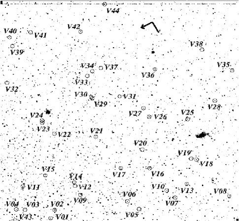
Figure 2: Finding charts for the And VI variable stars. The WFC2 ($1.2\arcmin$x$1.3\arcmin$), WFC3 ($1.3\arcmin$x$1.2\arcmin$), and WFC4 ($1.2\arcmin$x$1.2\arcmin$) images are each shown in a panel. North and east directions are shown with the arrow pointing toward the north.

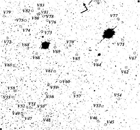
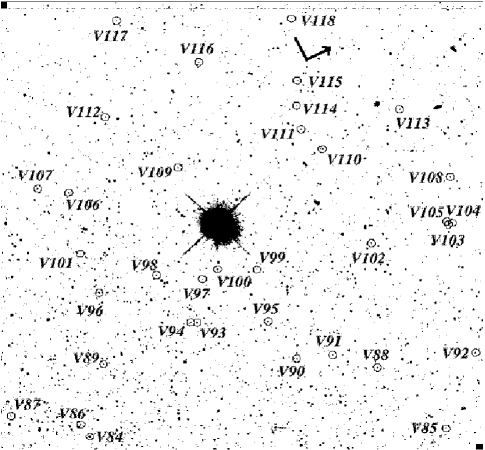
Figure 2 cont: Finding charts for the And VI variable stars. The WFC2 ($1.2\arcmin$x$1.3\arcmin$), WFC3 ($1.3\arcmin$x$1.2\arcmin$), and WFC4 ($1.2\arcmin$x$1.2\arcmin$) images are each shown in a panel. North and east directions are shown with the arrow pointing toward the north.

Figure 2 cont: Finding charts for the And VI variable stars. The WFC2 ($1.2\arcmin$x$1.3\arcmin$), WFC3 ($1.3\arcmin$x$1.2\arcmin$), and WFC4 ($1.2\arcmin$x$1.2\arcmin$) images are each shown in a panel. North and east directions are shown with the arrow pointing toward the north.

3.1 Variable Star Colors

Choosing the correct magnitude offset as discussed in §3 provided a challenge with the variable stars due to the varying brightness along the light curve. However, for RRL with uniform reddening, it is known that the colors during minimum light are approximately the same. With this in mind, we calibrated those stars for which we had photometry in both filters during minimum light. These variable stars fell within the expected instability strip, which is approximately $0.26<(\bv)<0.46$ given $E(\bv)=0.06$ from AJD99. Knowing what the magnitude offsets should look like from these variable stars, we were able to accurately calibrate the approximately 25% of the variable stars which only had photometry during minimum light for one filter.

In Figure 1 we show the location of the variables within the color-magnitude diagram. All variables lie within the instability strip with the RRL forming a distinct group along the horizontal branch, while the brighter stars are likely to be ACs. We investigated the stars scattered about the location of the ACs and found them to show no variability. It should be noted that the colors and magnitudes for all the stars have inherent uncertainties of order 0.02-0.03 mag due to the method we have used to calibrate the data to the $B$,$V$ system. Nevertheless, our approach is adequate to investigate the general properties of And VI as demonstrated in the following sections.

In Table 1 we present the photometric properties for the 118 variables while their photometric $B$ and $V$ data are in Tables 2 and 3. Column 1 of Table 1 lists the star’s ID, while the next two columns give the RA and Dec. Finding charts for the variables are found in Figure 2. Of these variables, 6 are likely ACs and they are discussed in the following section with their light curves shown in Figure 3. A further 111 are RRL and Figure 4 shows their light curves with their properties discussed in §5, with the exception of V103. The variable V103 only had photometry along the descending branch of the light curve. Therefore no templates adequately fit the data. We were unable to classify one candidate variable (V34). The best fit for the data implies that it is a contact binary. On the other hand, its magnitude and color place it among the RRL. For this reason we have not definitively classified this variable and have left it out of our analysis.

Figure 5: And VI anomalous Cepheid light curves with the observations shown as filled circles and the fitted template displayed as a curve.

Figure 6: And VI RR Lyrae light curves with the observations shown as filled circles and the fitted template displayed as a curve.

Figure 4 cont: And VI RR Lyrae light curves with the observations shown as filled circles and the fitted template displayed as a curve.

Figure 4 cont: And VI RR Lyrae light curves with the observations shown as filled circles and the fitted template displayed as a curve.

Figure 4 cont: And VI RR Lyrae light curves with the observations shown as filled circles and the fitted template displayed as a curve.

Figure 4 cont: And VI RR Lyrae light curves with the observations shown as filled circles and the fitted template displayed as a curve.

4 And VI Anomalous Cepheids

ACs are typically 0.5 - 1.5 mag brighter than the RRL in a system. This difference indicates that ACs have masses in the range of 1 - 2 $M_{\odot}$ (Norris & Zinn 1975; Zinn & Searle 1976; Zinn & King 1982; Smith & Stryker 1986; Bono et al. 1997b). In order for such stars to evolve into the instability strip, they are required to have low metallicities, approximately ${\rm[Fe/H]}<-1.3$ (Demarque & Hirshfeld 1975). Given that masses in excess of the turnoff mass of old globular clusters ($M>0.8~{}M_{\odot}$) are required, the two leading hypotheses for the origin of ACs are that they are either stars from an intermediate age population, age less than 5 Gyr (e.g., Demarque & Hirshfeld 1975; Norris & Zinn 1975), or stars of increased mass due to mass transfer in a binary system of older stars (Renzini, Mengel, & Sweigart 1977). Both scenarios are plausible. It may be the case that the origin of the ACs is tied to the system in which they originate. While there seems to be no clear way of selecting between the two origin scenarios, the most likely explanation for the ACs found in globular clusters, such as NGC 5466 (Zinn & Dahn 1976) and possibly $\omega$ Centauri (Wallerstein & Cox 1984), is the mass transfer scenario. For dSphs, both scenarios may be effective.

While ACs are almost nonexistent in globular clusters, they are common in dSphs. Every dSph surveyed for variable stars has been shown to include at least one AC. Thus it is not unexpected that And VI would contain at least one AC, especially given the mean metallicity of the dSph ($\langle{\rm[Fe/H]}\rangle=-1.58$, AJD99).

Six of the 118 variables found in this survey are likely ACs. Their photometric properties are listed in Table 1 and their light curves are shown in Figure 3. The first and fourth columns of Table 1 list the star’s identification along with its period. The intensity-weighted $\langle V\rangle$ and $\langle B\rangle$ magnitudes are given in the fifth and sixth columns. The magnitude-weighted B Vcolor, $(\bv)_{\rm mag}$, is listed in the seventh column. Columns eight and nine list the $V$ and $B$ amplitudes for the variables. The other columns will be discussed subsequently, but the classifications are in column twelve. We searched the literature for ACs with $(\bv)$ colors and found that they lie between the typical red and blue edges of the RRL instability strip. As can be seen in Figure 1, the And VI candidate ACs are consistent with the expected position for ACs in the CMD. For two ACs we were not able to make full use of the data. V44 was very near the edge of the WFC2 CCD in the second pointing, and so only photometry from the first pointing is available. For V83, the star fell near or on a bad column in the first pointing. This resulted in the loss of all the F450W data for this star at this pointing, though the F555W photometry was unaffected. Similarly, for the second pointing, we were able to only use two F555W and two F450W measurements for this star. As a result, the magnitudes and colors for V44 and V83 are less well determined than for the other variables. However, their periods and absolute magnitudes are consistent with those for the other ACs.

One way to classify the pulsation modes of variable stars is on the basis of the shape of their light curves. First-overtone mode stars typically have a more sinusoidal shape to their light curves, while fundamental mode stars have more asymmetric light curves. This is clearly seen in RRL and other Cepheid stars, but the case is not so clear for ACs. While some first-overtone mode ACs may have more sinusoidal light curves, others look “less asymmetric” than a light curve for a fundamental mode star. An example of this would be the difference between a RRa star, which has a sharp rise to maximum light, and a RRb star, which has a gentle rise to maximum light (Bailey 1902), though both are fundamental mode pulsators. On this basis, we can attempt to classify the ACs in And VI. And VI ACs pulsating in the fundamental mode are V06 and V84. First-overtone mode stars are V52 and V93. We are unable to definitively classify V44 and V83 due to the small number of points and difficulties with the photometry as stated above. On the other hand, the small number of points renders these classifications preliminary. For example, from the absolute magnitude versus the period of the ACs, V93 may well be pulsating in the fundamental mode (see §4.1).

4.1 Anomalous Cepheid Absolute Magnitudes

In order to compare the properties of the And VI ACs with those for other known ACs, we have converted the available photometry to absolute magnitudes. AJD99 derive an And VI distance modulus $(m-M)_{0}=24.45$ from the $I$ magnitude of the tip of the red giant branch. We have adopted this value together with their listed And VI reddening, $E(\bv)=0.06$ mag.

For the ACs in Galactic dSphs, we have adopted reddenings from Mateo (1998), while for the AC in the globular cluster NGC 5466 we have used the reddening from Harris (1996). In order to have all distance moduli on the same system, we have searched the literature for distance estimates derived from the tip of the red giant branch. For the cases where these estimates were not available, we used the mean magnitude of the RRL along with the absolute magnitude based on the Lee, Demarque, & Zinn distance scale (Eq. 7 of Lee, Demarque, & Zinn 1990) to calculate the distance modulus. The tip of the red giant branch method is based upon this distance scale. We have also adopted total-to-selective extinction ratios $R_{V}=3.1$ and $R_{B}=4.1$, respectively. The results are given in Table 4. Here the first column identifies the system while the second and third give the associated distance modulus and reddening. The ID for each AC and the mode of pulsation (F$=$fundamental mode; H$=$first-overtone mode) based on the position in the absolute magnitude versus the logarithm of the period diagram (see below) are given in columns 4 and 5, respectively, along with the period (column 6). Note that the IDs given for the ACs taken from Bersier & Wood (2002) only list the last three digits of the full IDs given in that paper. The mean apparent magnitudes and respective absolute magnitudes are listed in columns 7 through 10. Columns 11 and 12 list the $V$ and $B$ amplitudes for the ACs. In each case we have reviewed the original photometry to check the periods and magnitudes. Cases where we have made revisions to previous adopted values are indicated by an asterisk. We have not attempted to revise the Leo I data because of its generally poorer quality.

Figure 11: $M_{B}$ versus period for anomalous Cepheids. Figure (a) includes all available anomalous Cepheids and (b) leaves out the Carina and Leo I data. The solid lines in (b) are from Eqs. 13 and 14 from Bono et al. (1997b), while the dashed lines are from Eqs. 2 and 3 from this paper.

Figure 5 shows the $B$ absolute magnitudes for the ACs as a function of their period. In Figure 5a, which plots all available ACs, scatter is present in the plot and the difference between the two pulsational modes is not clear. Since there is significant scatter in the photographic light curves of the Carina and Leo I ACs, we have removed these ACs in Figure 5b. The difference between the pulsation modes is more evident in this plot. It is clear that the slopes for the two pulsation modes are not parallel. This contradicts the suggestion of Nemec, Nemec, & Lutz (1994) (cf. Figure 5), although the idea of non-parallel lines is in better agreement with the original analysis of Nemec, Wehlau, & Mendes de Oliveira (1988). The difference in slopes was also noted by Bono et al. (1997b) in their analysis of ACs based on the Nemec, Nemec, & Lutz data. Using Eqs. 13 and 14 of Bono et al., we have plotted these lines in Figure 5b for the different pulsational modes. The lines appear to be slightly fainter than the data. We have attempted to fit lines to the data in Figure 5b. Due to the fundamental and first-overtone ACs converging at short periods, there is some uncertainty in the classification of those variables. For the purposes of fitting the lines, we have left out V9 in Sextans since it is unclear whether it is pulsating in the fundamental or first-overtone mode. The equations for the resulting lines are:

$$M_{B,{\rm F}}=-2.62(\pm 0.18)\log\,P-0.40(\pm 0.04)$$ (2)

$$M_{B,{\rm H}}=-3.99(\pm 0.27)\log\,P-1.43(\pm 0.09)$$ (3)

The slopes for our lines match well with what was found by Bono et al., but the zeropoint is different, perhaps as a result of different adopted distance scales.

Figure 12: $M_{V}$ versus period for anomalous Cepheids. All data is included in (a) and the Fornax data from Bersier & Wood (2002) is removed in (b). The dashed lines in (b) are from Eqs. 4 and 5 from this paper.

In Figure 6 we have plotted $M_{V}$ versus period. Again, in Figure 6a we have included all available data. Much of the scatter is due to the Fornax ACs from Bersier & Wood (2002). Because of the high scatter in their light curves, we have left out these variables in Figure 6b. As for the $B$ data, we have fit lines to the data in Figure 6b. We again omit from the fit V9 in Sextans, and also V1 in Leo II for similar reasons which will be discussed in §4.2.

$$M_{V,{\rm F}}=-2.64(\pm 0.17)\log\,P-0.71(\pm 0.03)$$ (4)

$$M_{V,{\rm H}}=-3.74(\pm 0.20)\log\,P-1.61(\pm 0.07)$$ (5)

The slopes for these lines match well to those found for the $B$ AC data. We are not aware of any a priori reason why this should be true.

4.2 Anomalous Cepheid Period-Amplitude Diagram

In Figure 7 we plot the amplitudes versus log period for our sample of ACs. The Carina and Leo I ACs have been excluded from Figure 7a due to the large scatter in their photometry, while the Fornax ACs from Bersier & Wood (2002) have been left out of Figure 7b for similar reasons. The pulsation modes are assigned according to each variable’s positions in the $M-\log\,P$ diagrams. In Figure 7 there is no clear trend in $V$ or $B$ amplitude with pulsation mode. This is similar to what was found by Nemec, Nemec, & Lutz (1994, their Fig. 10). The same is not true for RRL where there are clear distinctions between pulsation modes in the period-amplitude diagram. For RRL, there is a clear break in period between fundamental mode, RRab, and first-overtone mode, RRc, stars with the longest period RRc star having a shorter period than the shortest period RRab star in a given system. This is due to the ionization zone being located deeper within the envelope for the bluer variables. A similar effect is seen in the classical Cepheids (e.g., Smith et al. 1992) where the first-overtone Cepheids tend to have lower amplitudes coupled with their shorter periods.

Bono et al. (1997b) used theoretical models to analyze the properties of ACs. They argued that the predicted location of the zero-age horizontal branch in the amplitude-$\log\,P$ diagram provided a transition between the fundamental mode pulsators and the first-overtone mode pulsators in the period-amplitude diagram. We have plotted this line in Figure 7b. Bono et al. stated that all ACs with period shorter than this line are pulsating in the first-overtone and those with longer periods are pulsating in the fundamental mode.

Taking a closer look at the fundamental mode ACs to the left of the Bono et al. line, the likely reasons for their being to the left of the line are either they have the wrong classification or their periods and/or amplitudes are incorrect. V6 from And VI is close enough to the line that we leave it out of further discussion. V93 from And VI is another one of the fundamental mode ACs to the left of the line. Due to the fundamental mode and first-overtone mode lines nearly intersecting as seen in Figures 5 and 6, it is possible that V93 is actually a first-overtone pulsator although it doesn’t seem likely. A better case may be made for V9 in Sextans. Still, there are a few other ACs (V1 and V56 of Ursa Minor and V055 and V208 of Draco) that are found among the first-overtone pulsators that appear to be pulsating in the fundamental mode according to their position in the absolute magnitude versus $\log\,P$ plots. In any case, more and better observations would likely help in better defining the period-amplitude diagrams.

5 And VI RR Lyrae

The presence of RRL within a system indicates the existence of an old population ($t>10$ Gyr). For And VI we have detected 111 RRL with 91 pulsating in the fundamental mode (RRab) and 20 pulsating in the first-overtone mode (RRc). There is one RRL (V103) which we were unable to place on the $B$,$V$ system due to a large gap in its light curve. As a result, its magnitude and amplitude were not used in the following results. Although our search for variables was extensive, the number of RRc stars is more than likely greater than what we found. The scatter in the photometry along with the low amplitude of the RRc star makes it difficult to detect this type of variable. A histogram of the RRL periods in And VI is compared to other dSphs in Figure 8, with the dSphs increasing in mean metallicity from the top, Ursa Minor, to the bottom, Fornax. The sources for the data are the same as those listed in Table 4. There is a clear trend in the populations of the RRab stars with the more metal-poor dSphs tending to have longer period RRab stars than the more metal-rich dSphs. There appears to be no obvious trend with the RRc stars. This may be due, in part, to the difficulty in detecting the smaller amplitude RRc stars, as we noted in this survey.

Figure 13: Period-amplitude diagram for anomalous Cepheids. First-overtone stars are denoted by open circles and fundamental mode stars are denoted by filled circles. Asterisks denote ACs with uncertain classification as noted in Table 4. Only anomalous Cepheids with good photometry are included in the $V$ (a) and $B$ (b) plots. The line in (b), taken from Figure 7 of Bono et al. (1997b), represents the predicted location of the zero-age horizontal branch fundamental mode pulsators, and is meant to divide fundamental mode from first-overtone pulsators.

Figure 14: Period distribution plots for the RR Lyrae in dwarf spheroidal galaxies. The [Fe/H] values were taken from Mateo (1998).

From the sample of RRL in And VI we find the mean magnitude to be $\langle V\rangle=25.29\pm 0.03$, where the uncertainty is the aperture correction uncertainty, the photometry zeropoint uncertainty, and the spline-fitting uncertainty added in quadrature to the standard error of the mean. In order to convert this RRL magnitude to a distance on the same scale as the tip of the red giant branch distance of AJD99, we calculated $M_{V}$ of the RRL from Lee, Demarque, & Zinn (1990),

$$M_{V,{\rm RR}}=0.17{\rm[Fe/H]}+0.82{\rm.}$$ (6)

Adopting $\langle{\rm[Fe/H]}\rangle=-1.58\pm 0.20$ and $E(\bv)=0.06\pm 0.01$ from AJD99, we find $M_{V,{\rm RR}}=0.55$ and $A_{V}=3.1E(\bv)=0.19\pm 0.03$. The resulting distance is $815\pm 25$ kpc. This matches up well with the tip of the red giant branch distance estimate by AJD99 of $775\pm 35$ kpc.

5.1 RR Lyrae Period-Amplitude Diagram

The period-amplitude diagram provides an important diagnostic tool when investigating the properties of a system as the period and the amplitude of a variable are independent of quantities such as distance and reddening. It is generally thought that the position of a RRL in the period-amplitude diagram is dependent on the metallicity of the star (Sandage 1993b). More recently, Clement et al. (2001) in a study of the properties of the RRL in Galactic globular clusters suggested that while this may be true for the more metal-rich Oosterhoff type I clusters, the same may not be true for the more metal–poor Oosterhoff type II clusters.

In Figure 9, we plot the RRL found in And VI in a period-amplitude ($A_{B}$) diagram. The RRL fall in the expected positions with the RRc stars at shorter periods and lower amplitudes as compared to the longer period RRab stars. The RRc stars appear to fall into a parabolic shape, an effect predicted by Bono et al. (1997a). The width seen in the RRab stars is similar to what is seen in other dSphs (e.g., Leo II: Siegel & Majewski 2000; Sculptor: Kaluzny et al. 1995). This is not unexpected since dSphs are known to have a spread in their metallicity (see Mateo 1998 and references therein). It is uncertain how much the And VI spread in metallicity ($\sigma({\rm[Fe/H]})\approx 0.3$, AJD99) may be the cause of the observed spread of the RRab stars in the period-amplitude diagram and how much may be due to other effects such as age or evolutionary effects.

Figure 15: Period-amplitude diagram for the RR Lyrae in And VI. The amplitudes shown are for the $B$ filter.

Figure 16: Period-amplitude diagram showing the linear regression fits to the RR Lyrae in dwarf spheroidal galaxies. Also shown are the linear regression fits to NGC 6934 and M53.

To allow comparison to other dSphs, we fit the RRab stars in the period-amplitude diagram by linear regression fits using the second equation from Table 1 of Isobe et al. (1990). This version of “least squares,” which places the dependence on the x-variable against the independent y-variable and accounts for uncertainties in both variables, gives the best fit visually to the data. Figure 10 plots the fits for And VI, Leo II (Siegel & Majewski 2000), Draco (Kinemuchi et al. 2002), and Sculptor (Kaluzny et al. 1995). For reference we also plotted the fits to two Oosterhoff clusters: NGC 6934 (Oosterhoff type I; Kaluzny, Olech, & Stanek 2001) and M53 (Oosterhoff type II; Kopacki 2000). These two clusters were chosen due to their well-defined data. It should be noted that these globular cluster lines are similar to the Oosterhoff lines defined by Clement (2000 and private communications). Table 5 lists the equations for each system. The fit for the RRab stars in And VI coincides with the fit for NGC 6934. This agrees with the idea that the position of RRab stars in a period-amplitude diagram is dependent on the metallicity since the metallicities of NGC 6934 (${\rm[Fe/H]}=-1.54$) and And VI ($\langle{\rm[Fe/H]}\rangle=-1.58$) are the same.

The fit of the Sculptor data, although slightly shifted toward longer periods, is found to be similar to the line for the more metal-rich NGC 6934. This is a bit surprising given the metallicity of Sculptor ($\langle{\rm[Fe/H]}\rangle=-1.8$). With [Fe/H] values of -2.0 and -1.9 for Draco and Leo II, respectively (Mateo 1998), one would expect the RRab stars to fall near the M53 (${\rm[Fe/H]}=-2.04$) line in Figure 10. Instead the fits to the data fall somewhere between NGC 6934 and M53 lines. The slopes of the lines for Leo II and Draco, while similar to each other are different from the slopes of And VI and Sculptor which also are similar to each other. Although the exact reason for the differences seen in the slopes and locations of the fits are uncertain, it is an effect that is seen in other dSphs, where the mean periods of the RRab stars in dSph systems do not follow the shift in period with abundance seen in Galactic GCs. We discuss this in the next section.

5.2 Oosterhoff Classification

Figure 17: The mean period for the RRab stars versus the metallicity of the parent system. Galactic globular clusters are shown as filled circles, along with $\omega$ Centauri (filled square). Large Magellanic Cloud globular clusters are shown as open triangles. The Galactic dwarf spheroidals are indicated by open circles. And VI is shown as an open square.

The RRab stars in metal-poor globular clusters have longer mean periods ($\langle P_{ab}\rangle=0.64$d) and higher ratios of RRc stars compared to the total number of RRL ($N_{c}/N_{RR}=0.44$) than do RRab stars in metal-rich clusters (Oosterhoff 1939) where $\langle P_{ab}\rangle=0.55$d and $N_{c}/N_{RR}=0.17$ (see Smith 1995 and references therein). Further, Galactic globular clusters having $-2.0<{\rm[Fe/H]}<-1.7$ contain few RRL because their horizontal branches lack stars in the vicinity of the instability strip. Although it is clear that metallicity is the first parameter governing the morphology of the horizontal branch and therefore the RRL content within the instability strip, secondary parameters (e.g., age, mass loss along the red giant branch, and rotation) also affect the horizontal branch morphology and thus confuse the general Oosterhoff trend.

RRL in the Galactic dSphs fall along a continuum within the Oosterhoff gap (van Agt 1973; Zinn 1978, 1985; Kaluzny et al. 1995; Mateo et al. 1995). A number of the Large Magellanic Cloud (LMC) globular clusters also fall within the Oosterhoff gap. In Table 6 we list the properties of the dSphs, including And VI, and the LMC globular clusters with at least 15 RRab stars whose light curves have minimum scatter and gaps in the data. For comparison, the mean properties for the Oosterhoff groups are also listed. The first two columns identify the various systems. The metallicities for the dSphs in the third column were taken from Mateo (1998; except for Leo I which is from Gallart et al. 1999), while the metallicities for the LMC GCs were taken from the literature. Columns 4 and 5 give the mean periods for the RRab and RRc stars and columns 6–8 give the number of RRab and RRc stars, along with the ratio of RRc stars to the total number of RRL. To better illustrate how these systems fill in the “intermediate” metallicities we have also plotted the logarithm of the mean RRab periods versus the metallicity of the parent system in Figure 11. We have left out the Sagittarius dSph since the precise metallicity related to the RRL is uncertain. Also plotted in the figure are Galactic globular clusters with at least 15 RRab stars (Clement et al. 2001 and references therein). Excluding $\omega$ Centauri, which has a spread in metallicity (e.g., Freeman & Rodgers 1975), and M2, which shows the second parameter effect (e.g., Lee & Carney 1999), the Oosterhoff dichotomy is clearly seen in the Galactic globular clusters as noted by Oosterhoff (1939). As discussed above, the properties of And VI are consistent with the Galactic dSphs. The one Galactic dSph that is somewhat offset from the other dSphs in Figure 11 is Fornax. Given the large age and abundance range in Fornax, it is possible that the mean [Fe/H] of the RRL is lower than that of the galaxy as a whole (see Bersier & Wood 2002). This effect would act to displace Fornax toward the other dSphs in Figure 11.

While studying M15 and M3, Sandage, Katem, and Sandage (1981) noticed a period shift between the RRL in these clusters in the period-amplitude diagram that correlated with metallicity (Sandage 1981;1982a,b). Metal-poor clusters tend to have longer periods for a given amplitude when compared to metal-rich clusters such that,

$$\Delta\log\,P=-(0.129A_{B}+0.088+\log\,P)$$ (7)

relative to M3 (Sandage 1982a,b). From Eq. 7, Oosterhoff type I clusters have $\langle\Delta\log\,P\rangle\geq-0.01$, while Oosterhoff type II clusters have $\langle\Delta\log\,P\rangle\leq-0.05$ and field RRL tend to avoid a range $-0.05\leq\Delta\log\,P\leq-0.01$ (Suntzeff et al. 1991).

RRL in dSphs, though, are found in the $-0.05\leq\Delta\log\,P\leq-0.01$ range (Sextans: Mateo et al. 1995; Leo II: Siegel & Majewski 2000). For And VI we calculated the $\Delta\log\,P$ values for the RRab stars, listed in column ten of Table 1, and plot them against $\log\,P$ in Figure 12. There are a number of stars in the region where Galactic RRab stars are absent. This shows that the “intermediate” mean periods of the RRab stars in dSphs are not a result of a superposition of Oosterhoff type I and II populations. Still, it is interesting to note that $\langle\Delta\log\,P\rangle=0.00$ for And VI arguing that there is no period shift compared to the Oosterhoff type I cluster, M3. Again, this is not unexpected since the metallicity of M3 (${\rm[Fe/H]}=-1.57$, Harris 1996) is the same as And VI ($\langle{\rm[Fe/H]}\rangle=-1.58$, AJD99).

Figure 18: The period shift versus period for the RRab stars in And VI. The dashed lines represent the zone in which few RRab stars from Galactic globular clusters are found.

It is easy to see from Table 6 that the mean periods of the RRab stars in the “intermediate” systems primarily follow the metallicity of the parent system. Therefore it is not surprising to see that $\langle P_{ab}\rangle$ for And VI is similar to the values found in Galactic globular clusters of similar [Fe/H]. This is consistent with our finding in §5.1 that the individual RRab stars in And VI fall along the line defined by the Oosterhoff type I cluster, NGC 6934 (${\rm[Fe/H]}=-1.54$, $\langle P_{ab}\rangle=0.574$d, Kaluzny et al. 2001).

The presence of systems within the gap between the Oosterhoff groups brings up questions regarding whether there is an Oosterhoff dichotomy as seen in Galactic globular clusters or an “Oosterhoff continuum” as seen in dSphs (Renzini 1983; Castellani 1983). The question is: What is the origin of the difference between systems such as the dSphs and LMC globular clusters that have significant numbers of RRL and the Galactic globular clusters in the same abundance range which have little or no RRL? Clearly, the presence of RRL in this metallicity range is due to the differences in the horizontal branch morphology between the systems. All dSphs with adequately deep CMDs, except Ursa Minor, exhibit the second parameter effect. The combined effects of metallicity spreads, in addition to extended periods of star formation (Mateo 1998), may explain the different horizontal branch morphology in the dSph systems. Yet it is unlikely this can be the explanation for the LMC globular clusters which have no metallicity spread and have been shown to have the same ages as their Galactic counterparts (Olsen et al. 1998; Johnson et al. 1999). Further observations of other systems within this metallicity range would help in clearing up this debate. In any case, the idea of metallicity being the first parameter governing the horizontal branch morphology and $\langle P_{ab}\rangle$ is clear in Figure 11.

5.3 Metallicity Estimates from RR Lyrae

A number of Galactic dSphs have been shown to exhibit a spread in their metallicities (see Mateo 1998 and references therein). Consequently, the exact metallicities for the individual RRL are uncertain. One method for determining the metallicity of the bulk of the RRL is through a relation determined by Alcock et al. (2000) relating the metallicity of a RRab star to its period and $V$-band amplitude. The relation,

$${\rm[Fe/H]}_{\rm ZW}=-8.85(\log\,P_{ab}+0.15A_{V})-2.60{\rm,}$$ (8)

was calibrated using the RRab stars in M3, M5, and M15, where ZW refers to the Zinn & West (1984) scale. Their calibration predicted the metallicity of the RRL in those systems with an accuracy of $\sigma_{\rm[Fe/H]}=0.31$ per star. Alcock et al. tested this formula on their sample of RRab stars from the LMC and found the resulting median metallicity to be in good agreement with previous results.

We list in column eleven of Table 1 the resulting metallicities for the individual RRab stars using Eq. 8. These results were plotted in the [Fe/H] distribution plot seen in Figure 13. A gaussian fit to the data reveals a mean metallicity of ${\rm[Fe/H]}=-1.58$ with a fitting error of 0.01 and a standard deviation of 0.33. This is exactly what was found by AJD99 ($\langle{\rm[Fe/H]}\rangle=-1.58\pm 0.20$) using the red giant branch mean $V$–$I$ color. Since the accuracy of the Alcock et al. equation is on the order of $\sim 0.3$ dex, there is no evidence for any abundance dispersion in the RRab stars given $\sigma=0.33$. We also investigated the distribution of ${\rm[Fe/H]}$ values with distance from the center of And VI and saw no convincing evidence for any metallicity gradient.

Figure 19: [Fe/H] distribution plot for the RRab stars in And VI. The individual [Fe/H] values were calculated using Eq. 2 in Alcock et al. (2000). The dashed line represents a gaussian fit to the data. The curve has a mean of ${\rm[Fe/H]}=-1.58$ and a standard deviation of 0.33.

Sandage (1993a) studied cluster and field RRL spanning a wide range of metallicities and related the average periods of RRL to their metallicities through the relations

$${\rm[Fe/H]}_{\rm ZW}=(-\log\,\langle\,P_{ab}\rangle-0.389)/0.092$$ (9)

$${\rm[Fe/H]}_{\rm ZW}=(-\log\,\langle\,P_{c}\rangle-0.670)/0.119$$ (10)

Siegel & Majewski (2000) and Cseresnjes (2001) showed that, although these relations were derived from cluster and field RRL, the RRL in dSphs follow the same relations. For And VI, $\langle P_{ab}\rangle=0.588\pm 0.005$d and $\langle P_{c}\rangle=0.382\pm 0.005$d resulting in ${\rm[Fe/H]}_{\rm ZW}=-1.72\pm 0.04$ (internal error) for the RRab stars and ${\rm[Fe/H]}_{\rm ZW}=-2.12\pm 0.05$ (internal error) for the RRc stars. The estimate derived from the RRab stars is slightly metal-poor when compared to the estimate derived from the Alcock et al. (2000) formula, but given the uncertainties in both methods, the values are not inconsistent with each other. The metallicity estimate from the RRc stars is much more metal-poor than what was derived from the RRab stars. This should be taken with some caution since as discussed in §5, our search for RRc stars is more than likely incomplete. As a result, the mean period for the RRc stars is probably inaccurate.

6 Summary & Conclusions

We have presented the light curves and photometric properties for 118 variables found in the And VI dwarf spheroidal galaxy. The properties of the variable stars in And VI were shown to be consistent with those found in other dSphs. In particular, the 6 anomalous Cepheids found in And VI have periods and absolute magnitudes similar to the anomalous Cepheids in other systems. We redetermined the period-luminosity relations for the anomalous Cepheids and concur with the previous results of Nemec, Wehlau, & Mendes de Oliveira (1988) and Bono et al. (1997b), that the lines representing the different pulsation modes are not parallel. Unlike the situation for RR Lyrae, we were not able to make a clear distinction between the fundamental and first-overtone mode anomalous Cepheids in a period-amplitude diagram.

From a sample of 110 RR Lyrae, we found the mean $V$ magnitude to be $25.29\pm 0.03$ resulting in a distance for And VI of $815\pm 25$ kpc on the Lee, Demarque, & Zinn (1990) distance scale. The mean period of the RRab stars in And VI, $\langle P_{ab}\rangle=0.588$d, is consistent with the galaxy’s mean metallicity of $\langle{\rm[Fe/H]}\rangle=-1.58$ and follows the trend of the Galactic dwarf spheroidal galaxies filling in the gap between the Oosterhoff groups. The location of the RRab stars in a period-amplitude diagram is consistent with Galactic globular clusters of similar metallicity. We were also able to show that a number of RR Lyrae metallicity indicators, such as Eq. 2 from Alcock et al. (2000) and the Sandage (1982a,b) period shift, give results consistent with the mean abundance ($\langle{\rm[Fe/H]}\rangle=-1.58\pm 0.20$) derived by AJD99 from the red giant branch. Indeed, based on the properties of its variable stars, the And VI dSph is indistinguishable from the Galactic dSph companions.

Table 1: Light Curve Properties

ID	RA (2000)	Dec (2000)	Period	$\langle V\rangle$	$\langle B\rangle$	$(B-V)_{\rm mag}$	$A_{V}$	$A_{B}$	$\Delta\log\,P$	[Fe/H]	Classification
V01	23:51:47.9	24:34:39.5	0.579	25.387	25.734	0.389	0.99	1.40	-0.03	-1.81	ab
V02	23:51:47.7	24:34:37.2	0.385	25.286	25.700	0.429	0.51	0.72	$\cdots$	$\cdots$	c
V03	23:51:47.4	24:34:45.1	0.434	25.217	25.570	0.362	0.41	0.57	$\cdots$	$\cdots$	c
V04	23:51:47.3	24:34:47.4	0.365	25.282	25.561	0.295	0.54	0.76	$\cdots$	$\cdots$	c
V05	23:51:48.6	24:34:14.0	0.427	25.255	25.665	0.414	0.28	0.40	$\cdots$	$\cdots$	c
V06	23:51:48.3	24:34:16.0	0.629	24.532	24.873	0.369	0.74	1.05	$\cdots$	$\cdots$	AC
V07	23:51:48.7	24:34:02.4	0.652	25.330	25.655	0.335	0.48	0.68	0.01	-1.59	ab
V08	23:51:49.2	24:33:47.5	0.590	25.209	25.491	0.299	0.64	0.90	0.03	-1.42	ab
V09	23:51:47.6	24:34:27.8	0.576	25.321	25.627	0.356	1.07	1.51	-0.04	-1.90	ab
V10	23:51:48.5	24:34:03.5	0.335	25.256	25.659	0.418	0.52	0.73	$\cdots$	$\cdots$	c
V11	23:51:46.9	24:34:42.0	0.534	25.125	25.352	0.256	0.82	1.17	0.03	-1.28	ab
V12	23:51:47.4	24:34:27.8	0.549	25.329	25.711	0.417	0.92	1.30	0.00	-1.52	ab
V13	23:51:48.5	24:33:57.0	0.395	25.132	25.385	0.266	0.46	0.65	$\cdots$	$\cdots$	c
V14	23:51:47.3	24:34:27.5	0.548	25.341	25.590	0.302	1.03	1.46	-0.02	-1.66	ab
V15	23:51:46.8	24:34:34.2	0.624	25.353	25.644	0.323	0.87	1.23	-0.04	-1.94	ab
V16	23:51:47.8	24:34:04.6	0.535	25.215	25.538	0.377	1.05	1.49	-0.01	-1.59	ab
V17	23:51:47.5	24:34:12.4	0.555	25.306	25.611	0.326	0.65	0.92	0.05	-1.20	ab
V18	23:51:48.1	24:33:50.4	0.532	25.119	25.421	0.341	0.96	1.36	0.01	-1.45	ab
V19	23:51:48.0	24:33:51.8	0.605	25.275	25.644	0.390	0.69	0.98	0.00	-1.58	ab
V20	23:51:47.3	24:34:03.5	0.591	25.267	25.656	0.415	0.73	1.03	0.01	-1.55	ab
V21	23:51:46.5	24:34:14.2	0.490	25.102	25.374	0.332	1.14	1.61	0.01	-1.37	ab
V22	23:51:46.0	24:34:25.0	0.519	25.130	25.400	0.308	0.94	1.34	0.02	-1.33	ab
V23	23:51:45.6	24:34:26.6	0.673	25.304	25.673	0.383	0.58	0.82	-0.02	-1.85	ab
V24	23:51:45.6	24:34:26.3	0.593	25.216	25.572	0.370	0.57	0.81	0.03	-1.35	ab
V25	23:51:47.1	24:33:46.3	0.626	25.338	25.710	0.397	0.78	1.11	-0.03	-1.84	ab
V26	23:51:46.6	24:33:56.4	0.512	25.306	25.658	0.417	1.12	1.58	0.00	-1.51	ab
V27	23:51:46.4	24:33:56.6	0.599	25.284	25.568	0.319	0.90	1.27	-0.03	-1.82	ab
V28	23:51:47.0	24:33:36.0	0.433	25.216	25.510	0.303	0.40	0.56	$\cdots$	$\cdots$	c
V29	23:51:45.6	24:34:09.0	0.536	25.104	25.356	0.297	1.02	1.44	0.00	-1.56	ab
V30	23:51:45.6	24:34:09.0	0.319	25.354	25.716	0.380	0.56	0.79	$\cdots$	$\cdots$	c
V31	23:51:45.9	24:34:01.2	0.647	25.161	25.567	0.423	0.59	0.83	-0.01	-1.71	ab
V32	23:51:44.4	24:34:29.7	0.717	25.224	25.522	0.309	0.49	0.69	-0.03	-1.97	ab
V33	23:51:45.1	24:34:06.7	0.567	25.183	25.494	0.341	0.83	1.18	0.01	-1.52	ab
V34	23:51:45.0	24:34:04.5	0.651	25.270	25.631	0.377	0.56	0.82	$\cdots$	$\cdots$	Contact Binary?
V35	23:51:46.5	24:33:26.5	0.604	25.237	25.595	0.385	0.81	1.14	-0.02	-1.74	ab
V36	23:51:45.6	24:33:47.1	0.539	25.406	25.682	0.331	1.12	1.58	-0.02	-1.71	ab
V37	23:51:45.0	24:34:01.7	0.691	25.362	25.674	0.330	0.64	0.91	-0.04	-2.03	ab
V38	23:51:45.7	24:33:31.3	0.548	25.143	25.507	0.402	0.87	1.23	0.01	-1.44	ab
V39	23:51:43.6	24:34:22.2	0.610	25.397	25.665	0.291	0.75	1.06	-0.01	-1.56	ab
V40	23:51:43.4	24:34:21.5	0.434	25.197	25.449	0.266	0.50	0.71	$\cdots$	$\cdots$	c
V41	23:51:43.5	24:34:15.1	0.512	25.145	25.466	0.376	1.12	1.59	0.00	-1.51	ab
V42	23:51:44.0	24:34:01.4	0.596	25.235	25.589	0.388	0.82	1.15	-0.01	-1.70	ab
V43	23:51:43.7	24:33:50.4	0.587	25.334	25.780	0.463	0.65	0.92	0.02	-1.42	ab
V44	23:51:47.5	24:34:49.4	0.760	23.624	23.988	0.378	0.53	0.75	$\cdots$	$\cdots$	AC
V45	23:51:43.5	24:34:32.8	0.546	25.340	25.553	0.266	1.09	1.55	-0.03	-1.72	ab
V46	23:51:43.7	24:34:36.3	0.652	25.307	25.546	0.251	0.49	0.70	0.01	-1.61	ab
V47	23:51:46.2	24:34:57.6	0.570	25.272	25.551	0.325	0.97	1.38	-0.02	-1.73	ab
V48	23:51:45.4	24:34:51.5	0.324	25.342	25.645	0.316	0.48	0.68	$\cdots$	$\cdots$	c
V49	23:51:46.2	24:34:59.1	0.545	25.340	25.677	0.411	1.20	1.60	-0.03	-1.86	ab
V50	23:51:45.5	24:34:56.5	0.614	25.364	25.717	0.363	0.52	0.73	0.03	-1.42	ab
V51	23:51:45.8	24:35:00.1	0.607	25.431	25.780	0.381	0.85	1.20	-0.03	-1.81	ab
V52	23:51:45.9	24:35:01.2	0.725	23.570	23.884	0.330	0.52	0.74	$\cdots$	$\cdots$	AC
V53	23:51:43.3	24:34:42.7	0.585	25.223	25.503	0.302	0.72	1.02	0.01	-1.50	ab
V54	23:51:42.5	24:34:42.3	0.518	25.382	25.603	0.257	0.82	1.17	0.05	-1.16	ab
V55	23:51:46.2	24:35:09.7	0.586	25.320	25.673	0.381	0.77	1.09	0.00	-1.57	ab
V56	23:51:45.0	24:35:03.2	0.556	25.367	25.694	0.368	0.89	1.26	0.00	-1.53	ab
V57	23:51:44.0	24:34:56.5	0.573	25.342	25.683	0.369	0.77	1.09	0.01	-1.48	ab
V58	23:51:46.0	24:35:12.2	0.654	25.363	25.651	0.301	0.52	0.74	0.00	-1.66	ab
V59	23:51:44.7	24:35:06.9	0.636	25.312	25.624	0.325	0.50	0.71	0.02	-1.52	ab
V60	23:51:44.2	24:35:05.6	0.590	25.398	25.803	0.433	0.81	1.15	-0.01	-1.65	ab
V61	23:51:44.2	24:35:12.3	0.527	25.487	25.846	0.394	0.87	1.22	0.03	-1.29	ab
V62	23:51:41.7	24:34:56.4	0.644	25.235	25.551	0.343	0.80	1.13	-0.04	-1.97	ab
V63	23:51:45.6	24:35:25.3	0.651	25.290	25.595	0.342	0.93	1.32	-0.07	-2.18	ab
V64	23:51:42.6	24:35:07.3	0.541	25.208	25.471	0.280	0.57	0.81	0.07	-1.00	ab
V65	23:51:43.2	24:35:15.1	0.412	25.271	25.538	0.276	0.40	0.57	$\cdots$	$\cdots$	c
V66	23:51:44.5	24:35:25.8	0.633	25.383	25.708	0.360	0.91	1.24	-0.01	-1.77	ab
V67	23:51:41.1	24:35:01.4	0.415	25.161	25.523	0.368	0.32	0.45	$\cdots$	$\cdots$	c
V68	23:51:44.8	24:35:30.7	0.594	25.103	25.408	0.330	0.72	1.03	0.01	-1.55	ab
V69	23:51:43.7	24:35:24.4	0.353	25.239	25.606	0.385	0.56	0.79	$\cdots$	$\cdots$	c
V70	23:51:43.2	24:35:21.3	0.529	25.296	25.681	0.442	1.08	1.53	-0.01	-1.59	ab
V71	23:51:41.3	24:35:10.8	0.546	25.300	25.720	0.451	0.79	1.12	0.03	-1.32	ab
V72	23:51:45.3	24:35:40.9	0.578	25.468	25.720	0.274	0.68	0.96	0.03	-1.40	ab
V73	23:51:43.9	24:35:35.6	0.660	25.321	25.578	0.269	0.52	0.74	0.00	-1.69	ab
V74	23:51:44.6	24:35:43.2	0.562	25.273	25.532	0.328	1.14	1.62	-0.01	-1.58	ab
V75	23:51:44.3	24:35:45.2	0.599	25.355	25.760	0.434	0.83	1.17	-0.02	-1.73	ab
V76	23:51:43.5	24:35:39.8	0.528	25.257	25.523	0.298	0.80	1.13	0.04	-1.21	ab
V77	23:51:41.0	24:35:22.7	0.569	25.395	25.738	0.364	0.72	1.02	0.03	-1.39	ab
V78	23:51:43.6	24:35:42.9	0.480	25.331	25.738	0.450	1.01	1.43	0.05	-1.12	ab
V79	23:51:45.0	24:35:52.7	0.639	25.399	25.704	0.313	0.43	0.61	0.03	-1.45	ab
V80	23:51:43.7	24:35:44.9	0.381	25.354	25.635	0.295	0.47	0.67	$\cdots$	$\cdots$	c
V81	23:51:43.7	24:35:45.3	0.386	25.361	25.628	0.285	0.56	0.79	$\cdots$	$\cdots$	c
V82	23:51:43.8	24:35:48.3	0.554	25.372	25.804	0.447	0.60	0.84	0.06	-1.13	ab
V83	23:51:43.6	24:35:47.7	0.674	23.471	23.789	0.332	0.50	0.70	$\cdots$	$\cdots$	AC
V84	23:51:47.2	24:35:10.6	1.357	23.661	24.054	0.408	0.60	0.84	$\cdots$	$\cdots$	AC
V85	23:51:45.4	24:35:59.9	0.651	25.243	25.683	0.457	0.64	0.90	-0.02	-1.80	ab
V86	23:51:47.3	24:35:10.3	0.307	25.254	25.683	0.436	0.36	0.51	$\cdots$	$\cdots$	c
V87	23:51:47.8	24:35:01.5	0.599	25.372	25.764	0.417	0.75	1.05	0.00	-1.63	ab
V88	23:51:46.4	24:35:55.1	0.621	25.383	25.651	0.282	0.58	0.82	0.01	-1.54	ab
V89	23:51:47.9	24:35:17.9	0.627	25.360	25.690	0.351	0.67	0.94	-0.01	-1.70	ab
V90	23:51:46.9	24:35:44.8	0.415	25.119	25.378	0.282	0.63	0.89	$\cdots$	$\cdots$	c
V91	23:51:46.8	24:35:50.0	0.349	25.364	25.601	0.255	0.55	0.78	$\cdots$	$\cdots$	c
V92	23:51:46.1	24:36:09.7	0.661	25.364	25.737	0.391	0.58	0.81	-0.01	-1.78	ab
V93	23:51:47.8	24:35:33.8	0.477	24.749	25.130	0.402	0.60	0.84	$\cdots$	$\cdots$	AC
V94	23:51:47.9	24:35:33.0	0.579	25.292	25.675	0.411	0.75	1.06	0.01	-1.50	ab
V95	23:51:47.5	24:35:43.7	0.548	25.284	25.629	0.389	0.93	1.31	0.05	-1.52	ab
V96	23:51:48.7	24:35:22.7	0.674	25.204	25.634	0.445	0.56	0.79	-0.02	-1.83	ab
V97	23:51:48.3	24:35:37.8	0.614	25.371	25.658	0.326	0.96	1.37	-0.05	-2.01	ab
V98	23:51:48.6	24:35:31.8	0.563	25.344	25.710	0.385	0.67	0.95	0.04	-1.28	ab
V99	23:51:48.1	24:35:46.0	0.608	25.358	25.774	0.443	0.80	1.13	-0.02	-1.75	ab
V100	23:51:48.3	24:35:40.6	0.666	25.215	25.588	0.386	0.54	0.77	-0.01	-1.75	ab
V101	23:51:49.2	24:35:23.0	0.595	25.292	25.675	0.402	0.62	0.88	0.02	-1.43	ab
V102	23:51:47.8	24:36:03.7	0.621	25.371	25.755	0.401	0.63	0.88	0.01	-1.61	ab
V103	23:51:47.6	24:36:15.6	0.734	$\cdots$	$\cdots$	$\cdots$	$\cdots$	$\cdots$	$\cdots$	$\cdots$	ab
V104	23:51:47.6	24:36:16.2	0.524	25.299	25.635	0.373	0.87	1.24	0.03	-1.27	ab
V105	23:51:47.7	24:36:15.6	0.524	25.141	25.415	0.322	0.95	1.35	0.02	-1.38	ab
V106	23:51:49.9	24:35:26.0	0.544	25.312	25.745	0.469	0.88	1.24	0.02	-1.43	ab
V107	23:51:50.1	24:35:22.2	0.590	25.457	25.752	0.335	0.88	1.25	-0.02	-1.74	ab
V108	23:51:48.1	24:36:19.4	0.572	25.339	25.714	0.403	0.74	1.05	0.02	-1.44	ab
V109	23:51:49.6	24:35:42.9	0.406	25.237	25.623	0.396	0.42	0.59	$\cdots$	$\cdots$	c
V110	23:51:49.1	24:36:04.1	0.636	25.313	25.715	0.414	0.51	0.73	0.01	-1.54	ab
V111	23:51:49.4	24:36:02.6	0.698	25.284	25.592	0.319	0.51	0.72	-0.02	-1.90	ab
V112	23:51:50.5	24:35:36.8	0.597	25.276	25.655	0.405	0.80	1.13	-0.01	-1.68	ab
V113	23:51:49.1	24:36:17.6	0.509	25.374	25.792	0.454	0.90	1.27	0.04	-1.20	ab
V114	23:51:49.7	24:36:03.7	0.619	25.207	25.523	0.343	0.73	1.03	-0.01	-1.73	ab
V115	23:51:49.9	24:36:05.7	0.572	25.360	25.719	0.377	0.67	0.94	0.03	-1.34	ab
V116	23:51:50.6	24:35:53.7	0.583	25.209	25.490	0.312	0.85	1.20	-0.01	-1.65	ab
V117	23:51:51.5	24:35:45.5	0.366	25.226	25.631	0.417	0.65	0.46	$\cdots$	$\cdots$	c
V118	23:51:50.6	24:36:09.5	0.511	25.203	25.476	0.293	0.71	1.00	0.07	-0.96	ab

Table 2: Photometry of the Variable Stars ($B$)

	V01			V02
HJD-2451000	$B$	$\sigma_{B}$		$B$	$\sigma_{B}$
476.729	26.078	0.208		26.150	0.342
476.746	25.592	0.214		25.973	0.213
476.797	24.883	0.100		25.524	0.113
476.813	25.130	0.156		25.453	0.238
476.863	25.418	0.235		$\cdots$	$\cdots$
476.880	25.498	0.164		25.273	0.123
476.931	25.654	0.223		25.545	0.146
476.947	25.734	0.179		25.687	0.112
479.011	26.249	0.210		25.861	0.138
479.028	26.243	0.236		26.161	0.195
479.078	25.126	0.145		25.784	0.134
479.095	25.099	0.193		25.658	0.115
479.146	25.227	0.094		25.491	0.106
479.162	25.253	0.207		25.214	0.113
479.213	25.553	0.143		$\cdots$	$\cdots$
479.230	25.627	0.175		25.458	0.152

Note. — The complete version of this table is in the electronic edition of the Journal. The printed edition contains only a sample.

Table 3: Photometry of the Variable Stars ($V$)

	V01			V02
HJD-2451000	$V$	$\sigma_{V}$		$V$	$\sigma_{V}$
476.597	25.763	0.085		25.316	0.101
476.613	25.767	0.206		25.451	0.075
476.661	25.772	0.208		25.450	0.102
476.677	25.658	0.197		25.539	0.129
478.879	25.557	0.087		25.332	0.131
478.895	25.789	0.120		25.508	0.173
478.943	25.580	0.100		25.392	0.154
478.960	25.511	0.151		25.576	0.127

Note. — The complete version of this table is in the electronic edition of the Journal. The printed edition contains only a sample.

Table 4: Properties of Anomalous Cepheids

System	$(m-M)_{0}$	E(B V)	ID	Mode	Period	$\langle V\rangle$	$\langle B\rangle$	$M_{V}$	$M_{B}$	$A_{V}$	$A_{B}$	References
And VI	24.45	0.06	6	F	0.629	24.53	24.87	–0.10	0.18	0.74	1.05	AJD99
			44	H	0.760	23.62	23.99	–1.01	–0.71	0.53	0.75
			52	H	0.725	23.57	23.88	–1.07	–0.81	0.52	0.74
			83	H	0.674	23.47	23.79	–1.17	–0.91	0.50	0.70
			84	F	1.357	23.66	24.05	–0.98	–0.64	0.60	0.84
			93	F	0.477	24.75	25.13	0.11	0.43	0.60	0.84
Leo I	21.93	0.01	1	F	1.322	$\cdots$	20.7	$\cdots$	–1.3	$\cdots$	1.6	HW78
			2	F	1.824	$\cdots$	21.0	$\cdots$	–1.0	$\cdots$	1.5
			8	F	2.374	$\cdots$	20.1	$\cdots$	–1.9	$\cdots$	1.0
			10	F	2.301	$\cdots$	21.0	$\cdots$	–1.0	$\cdots$	2.0
			11	H	0.851	$\cdots$	21.2	$\cdots$	–0.8	$\cdots$	0.7
			13	F	0.956	$\cdots$	21.8	$\cdots$	–0.2	$\cdots$	1.1
			15	F	1.024	$\cdots$	21.6	$\cdots$	–0.4	$\cdots$	1.2
			16	F	1.499	$\cdots$	20.9	$\cdots$	–1.1	$\cdots$	2.3
			17	H	0.799	$\cdots$	20.6	$\cdots$	–1.4	$\cdots$	1.5
			19	F	1.629	$\cdots$	20.7	$\cdots$	–1.3	$\cdots$	1.0
			20	F	1.522	$\cdots$	21.3	$\cdots$	–0.7	$\cdots$	1.0
			23	F	1.100	$\cdots$	21.4	$\cdots$	–0.6	$\cdots$	0.7
Leo II	21.59	0.02	1*	F?	0.408	21.97	$\cdots$	0.31	$\cdots$	0.76	$\cdots$	SM00
			27	F	1.486	20.45	$\cdots$	–1.20	$\cdots$	1.24	$\cdots$
			51*	H	0.396	21.59	$\cdots$	–0.06	$\cdots$	0.77	$\cdots$
			203	F	1.380	20.59	$\cdots$	–1.06	$\cdots$	1.05	$\cdots$
Draco	19.49	0.03	055	F	0.552	19.44	$\cdots$	–0.14	$\cdots$	0.57	$\cdots$	ZS76; K02
			119	F	0.907	19.03	$\cdots$	–0.55	$\cdots$	1.00	$\cdots$
			134	H	0.592	18.78	19.06	–0.79	–0.54	0.88	1.13
			141	F	0.901	19.12	19.43	–0.46	–0.17	0.72	1.15
			157	F	0.936	18.77	19.24	–0.80	–0.36	1.04	1.35
			194	F	1.590	18.12	18.53	–1.45	–1.07	0.46	0.52
			204	H	0.454	19.24	19.49	–0.33	–0.11	0.78	1.02
			208	F	0.608	19.28	$\cdots$	–0.29	$\cdots$	0.33	$\cdots$
Ursa Minor	19.16	0.03	1	F	0.471	$\cdots$	19.70	$\cdots$	0.42	$\cdots$	1.05	NWM88
			6	H	0.724	$\cdots$	18.25	$\cdots$	–1.03	$\cdots$	0.66
			11*	F	0.675	$\cdots$	19.29	$\cdots$	0.01	$\cdots$	1.59
			56	F	0.611	$\cdots$	19.38	$\cdots$	0.10	$\cdots$	0.48
			59	H	0.390	$\cdots$	19.56	$\cdots$	0.28	$\cdots$	1.01
			62*	H	0.421	$\cdots$	19.33	$\cdots$	0.05	$\cdots$	1.17
Carina	20.14	0.04	1	F	0.611	$\cdots$	20.20	$\cdots$	–0.10	$\cdots$	0.51	SMS86
			14	H	0.480	$\cdots$	20.11	$\cdots$	–0.19	$\cdots$	0.89
			27	H	0.511	$\cdots$	19.37	$\cdots$	–0.93	$\cdots$	1.68
			29	H	0.726	$\cdots$	19.20	$\cdots$	–1.10	$\cdots$	1.19
			33	F?	0.575	$\cdots$	20.16	$\cdots$	–0.14	$\cdots$	0.91
			129	H	0.640	$\cdots$	19.29	$\cdots$	–1.01	$\cdots$	0.99
			149	H	0.465	$\cdots$	20.31	$\cdots$	0.01	$\cdots$	1.30
Sculptor	19.56	0.02	26	F	1.346	18.55	$\cdots$	–1.08	$\cdots$	0.80	$\cdots$	K95
			119	F	1.159	18.86	$\cdots$	–0.76	$\cdots$	0.55	$\cdots$
			5689	F	0.855	19.14	$\cdots$	–0.47	$\cdots$	0.70	$\cdots$
Fornax	20.70	0.03	1	F	0.785	20.38	$\cdots$	–0.41	$\cdots$	0.95	$\cdots$	LAZ86
			825	F	1.045	19.80	$\cdots$	–0.99	$\cdots$	$\cdots$	$\cdots$	BW02
			012	F	1.250	19.91	$\cdots$	–0.89	$\cdots$	$\cdots$	$\cdots$
			316	F	0.508	20.79	$\cdots$	–0.01	$\cdots$	$\cdots$	$\cdots$
			122	F	0.504	20.83	$\cdots$	0.04	$\cdots$	$\cdots$	$\cdots$
			621	F	0.546	20.65	$\cdots$	–0.15	$\cdots$	$\cdots$	$\cdots$
			125	F	0.573	20.62	$\cdots$	–0.18	$\cdots$	$\cdots$	$\cdots$
			001	F	0.922	20.57	$\cdots$	–0.23	$\cdots$	$\cdots$	$\cdots$
			340	F	1.311	20.25	$\cdots$	–0.54	$\cdots$	$\cdots$	$\cdots$
			433	F	0.611	20.85	$\cdots$	0.05	$\cdots$	$\cdots$	$\cdots$
			601	F	0.574	21.02	$\cdots$	0.23	$\cdots$	$\cdots$	$\cdots$
			846	H?	0.416	20.83	$\cdots$	0.04	$\cdots$	$\cdots$	$\cdots$
			928	H	0.533	20.36	$\cdots$	–0.43	$\cdots$	$\cdots$	$\cdots$
			641	F	0.533	20.84	$\cdots$	0.05	$\cdots$	$\cdots$	$\cdots$
			024	F	1.198	19.99	$\cdots$	–0.80	$\cdots$	$\cdots$	$\cdots$
			802	F	0.838	20.48	$\cdots$	–0.31	$\cdots$	$\cdots$	$\cdots$
			335	F	0.506	20.83	$\cdots$	0.03	$\cdots$	$\cdots$	$\cdots$
			552	F	0.481	20.79	$\cdots$	–0.01	$\cdots$	$\cdots$	$\cdots$
Sextans	19.74	0.03	1	H	0.693	18.83	19.08	–1.00	–0.79	0.83	1.11	MFK95
			5	F	0.861	19.54	19.85	–0.30	–0.10	0.79	1.18
			6	F	0.922	19.19	19.46	–0.65	–0.40	1.31	1.64
			9*	F?	0.416	20.01	20.30	0.18	0.44	0.72	0.82
NGC 5466	16.03	0.00	19	H	0.822	14.731	14.909	–1.30	–1.12	0.60	0.70	CCN99

Note. — AJD99 = Armandroff, Jacoby & Davies (1999); HW78 = Hodge & Wright (1978); SM00 = Siegel & Majewski (2000); ZS76 = Zinn & Searle (1976); K02 = Kinemuchi et al. (2002); NWM88 = Nemec, Wehlau, & Mendes de Oliveira (1988); SMS86 = Saha, Monet, & Seitzer (1986); K95 = Kaluzny et al. (1995); LAZ86 = Light, Armandroff, & Zinn (1986); BW02 = Bersier & Wood (2002); MFK95 = Mateo, Fischer, & Krzeminski (1995); CCN99 = Corwin, Carney, & Nifong (1999)

Table 5: Period–Amplitude Fits for the RR Lyrae

System	Amplitude ($V$) Equation
Andromeda VI	$-7.036(\pm 0.719)\log\,P-0.860(\pm 0.170)$
Sculptor	$-5.885(\pm 0.468)\log\,P-0.544(\pm 0.109)$
Leo II	$-10.420(\pm 1.178)\log\,P-1.445(\pm 0.253)$
Draco	$-9.328(\pm 0.738)\log\,P-1.222(\pm 0.159)$

Table 6: Properties of RR Lyrae in Various Systems

	System	[Fe/H]	$\langle P_{ab}\rangle$	$\langle P_{c}\rangle$	$N_{ab}$	$N_{c}$	$N_{c}/N_{RR}$	Source
dSphs	Ursa Minor	-2.2	0.638	0.375	47	35	0.43	Nemec, Wehlau, & Mendes de Oliveira 1988
	Carina	-2.0	0.620	0.348	49	9	0.16	Saha, Monet, & Seitzer 1986
	Draco	-2.0	0.615	0.372	209	28	0.12	Kinemuchi et al. 2002
	Leo II	-1.9	0.619	0.363	92	30	0.25	Siegel & Majewski 2000
	Sculptor	-1.8	0.586	0.336	134	88	0.40	Kaluzny et al. 1995
	Sextans	-1.7	0.606	0.355	26	7	0.21	Mateo, Fischer, & Krzeminski 1995
	Leo I	-1.7	0.602	$\cdots$	63	11	0.15	Held et al. 2001
	Andromeda VI	-1.6	0.588	0.382	90	20	0.18	This Paper
	Fornax	-1.3	0.585	0.349	396	119	0.23	Bersier & Wood 2002
	Sagittarius	-1.0	0.574	0.322	$\cdots$	$\cdots$	$\cdots$	Cseresnjes 2001
LMC GCs	NGC 1841	-2.2	0.676	0.344	17	5	0.23	Kinman, Stryker, & Hesser 1976; Walker 1990
	NGC 2210	-1.9	0.598	0.379	20	9	0.31	Reid & Freedman 1994
	NGC 1466	-1.9	0.589	0.345	19	13	0.41	Walker 1992b
	NGC 1835	-1.8	0.598	0.326	18	15	0.46	Graham & Ruiz 1974; Walker 1993
	NGC 2257	-1.8	0.578	0.343	13	13	0.50	Walker 1989
	GLC 0435-59	-1.7	0.559	0.340	16	7	0.30	Walker 1992a
Oosterhoff	Type I	$\cdots$	0.55	0.32	$\cdots$	$\cdots$	0.17	Smith 1995
	Type II	$\cdots$	0.64	0.37	$\cdots$	$\cdots$	0.44	Smith 1995

References

- Alcock et al. (2000) Alcock, C., et al. 2000, AJ, 119, 2194
- Armandroff, Jacoby, & Davies (1999) Armandroff, T. E., Jacoby, G. H., & Davies, J. E. 1999, AJ, 118, 1220 (AJD99)
- Armandroff et al. (2002) Armandroff, T. E., et al. 2002, in preparation
- Bailey (1902) Bailey, S. I. 1902, Harv. Coll. Observ. Annals, 38, 1
- Bersier & Wood (2002) Bersier, D., & Wood, P. R. 2002, AJ, 123, 840
- Bono et al. (1997a) Bono, G., Caputo, F., Castellani, V., & Marconi, M. 1997a, A&AS, 121, 327
- Bono et al. (1997b) Bono, G., Caputo, F., Santolamazza, P., Cassisi, S., & Piersimoni, A. 1997b, AJ, 113, 2209
- Castellani (1983) Castellani, V. 1983, Mem. S. A. It., 54, 141
- Clement (2000) Clement, C. 2000, in The Impact of Large-Scale Surveys on Pulsating Star Research, ed. L. Szabados & D. W. Kurtz (San Francisco: ASP), 266
- Clement et al. (2001) Clement, C., et al. 2001, AJ, 122, 2587
- Corwin, Carney, & Nifong (1999) Corwin, T. M., Carney, B. W., & Nifong, B. G. 1999, AJ, 118, 2875
- Cseresnjes (2001) Cseresnjes, P. 2001, A&A, 375, 909
- Da Costa (1998) Da Costa, G. S. 1998, in Stellar Astrophysics for the Local Group, ed. A. Aparicio, A. Herrero, & F. Sanchez (Cambridge: Cambridge University Press), 351
- Demarque & Hirshfeld (1975) Demarque, P., & Hirshfeld, A. W. 1975, ApJ, 202, 346
- Dolphin (2000) Dolphin, A. E. 2000, PASP, 112, 1397
- Freeman & Rodgers (1975) Freeman, K. C., & Rodgers, A. W. 1975, ApJ, 201, L71
- Gallart et al. (1999) Gallart, C., Freedman, W. L., Aparicio, A., Bertelli, G., & Chiosi, C. 1999, AJ, 118, 2245
- Graham & Ruiz (1974) Graham, J. A., & Ruiz, M. T. 1974, AJ, 79, 363
- Grebel (1999) Grebel, E. K. 1999, in The Stellar Content of Local Group Galaxies, ed. P. Whitelock & R. Cannon (San Francisco: ASP), 17
- Harris (1996) Harris, W. E. 1996, AJ, 112, 1487
- Held et al. (2001) Held, E. V., Clementini, G., Rizzi, L., Momany, Y., Saviane, I., & Di Fabrizio, L. 2001, ApJ, 562, L39
- Hodge & Wright (1978) Hodge, P. W., & Wright, F. W. 1978, AJ, 83, 228
- Holtzman, J., et al. (1995) Holtzman, J. et al. 1995, PASP, 107, 1065
- Isobe et al. (1990) Isobe, T., Feigelson, E. D., Akritas, M. G., & Babu, G. J. 1990, ApJ, 364, 104
- Johnson et al. (1999) Johnson, J. A., Bolte, M., Stetson, P. B., Hesser, J. E., & Somerville, R. S. 1999, ApJ, 527, 199
- Kaluzny et al. (1995) Kaluzny, J., Kubiak, M., Szymanski, M., Udalski, A., Krzeminski, W., & Mateo, M. 1995, A&AS, 112, 407
- Kaluzny et al. (2001) Kaluzny, J., Olech, A., & Stanek, K. Z. 2001, AJ, 121, 1533
- Kinemuchi et al. (2002) Kinemuchi, K., Smith, H. A., LaCluyzé, A. P., Clark, H. C., Harris, H. C., Silbermann, N., & Snyder, L. A. 2002, in Radial and Nonradial Pulsations as Probes of Stellar Physics, ed. C. Aerts, T. R. Bedding, & J. Christensen-Dalsgaard (Cambridge: Cambridge University Press), in press (astro-ph/0203261)
- Kinman, Stryker, & Hesser (1976) Kinman, T. D., Stryker, L. L., & Hesser, J. E. 1976, PASP, 88, 393
- Klypin et al. (1999) Klypin, A., Kravtsov, A. V., Valenzuela, O., & Prada, F. 1999, ApJ, 522, 82
- Kopacki (2000) Kopacki, G. 2000, A&A, 358, 547
- Layden & Sarajedini (2000) Layden, A. C., & Sarajedini, A. 2000, AJ, 119, 1760
- Lee & Carney (1999) Lee, J.-W., & Carney, B. W. 1999, AJ, 118, 1373
- Lee, Demarque, & Zinn (1990) Lee, Y. W., Demarque, P., & Zinn, R. 1990, ApJ, 350, 155
- Light, Armandroff, & Zinn (1986) Light, R. M., Armandroff, T. E., & Zinn, R. 1986, AJ, 92, 43
- Mateo (1998) Mateo, M. 1998, ARA&A, 36, 435
- Mateo, Fischer, & Krzeminski (1995) Mateo, M., Fischer, P., & Krzeminski, W. 1995, AJ, 110, 2166
- Nemec, Nemec, & Lutz (1994) Nemec, J. M., Nemec, A. F. L., & Lutz, T. E. 1994, AJ, 108, 222
- Nemec, Wehlau, & Mendes de Oliveira (1988) Nemec, J. M., Wehlau, A., & Mendes de Oliveira, C. 1988, AJ, 96, 528
- Norris & Zinn (1975) Norris, J., & Zinn, R. 1975, ApJ, 202, 335
- Olsen et al. (1998) Olsen, K. A. G., Hodge, P. W., Mateo, M., Olszewski, E. W., Schommer, R. A., Suntzeff, N. B., & Walker, A. R. 1998, MNRAS, 300, 665
- Oosterhoff (1939) Oosterhoff, P. Th. 1939, Observatory, 62, 104
- Reid & Freedman (1994) Reid, N., & Freedman, W. 1994, MNRAS, 267, 821
- Renzini (1983) Renzini, A. 1983, Mem. S. A. It., 54, 335
- Renzini, Mengel, & Sweigart (1977) Renzini, A., Mengel, J. G., & Sweigart, A. V. 1977, A&A, 56, 369
- Saha, Monet, & Seitzer (1986) Saha, A., Monet, D. G., & Seitzer, P. 1986, AJ, 92, 302
- Sandage (1981) Sandage, A. 1981, ApJ, 248, 161
- Sandage (1982a) Sandage, A. 1982a, ApJ, 252, 553
- Sandage (1982b) Sandage, A. 1982b, ApJ, 252, 574
- Sandage (1993a) Sandage, A. 1993a, AJ, 106, 687
- Sandage (1993b) Sandage, A. 1993b, AJ, 106, 703
- Sandage, Katem, & Sandage (1981) Sandage, A., Katem, B., & Sandage, M. 1981, ApJS, 46, 41
- Siegel & Majewski (2000) Siegel, M. H., & Majewski, S. R. 2000, AJ, 120, 284
- Smith (1995) Smith, H. A. 1995, RR Lyrae Stars, (Cambridge: Cambridge University Press)
- Smith et al. (1992) Smith, H. A., Silbermann, N. A., Baird, S. R., & Graham, J. A. 1992, AJ, 104, 1430
- Smith & Stryker (1986) Smith, H. A., & Stryker, L. L. 1986, AJ, 92, 328
- Stetson (1992) Stetson, P. B. 1992, in Astronomical Data Analysis Software and Systems I, ed. D. M. Worrall, C. Biemesderfer, & J. Barnes (San Francisco: ASP), 297
- Stetson (1994) Stetson, P. B. 1994, PASP, 106, 250
- Stetson (1998) Stetson, P. B. 1998, PASP, 110, 1448
- Stetson et al. (1998) Stetson, P. B., et al. 1998, ApJ, 508, 491
- Suntzeff et al. (1991) Suntzeff, N. B., Kinman, T. D., & Kraft, R. P. 1991, ApJ, 367, 528
- van Agt (1973) van Agt, S. 1973, in Variable Stars in Globular Clusters and in Related Systems, ed. J. D. Fernie (Reidel: Dordrecht), 35
- Walker (1989) Walker, A. R. 1989, AJ, 98, 2086
- Walker (1990) Walker, A. R. 1990, AJ, 100, 1532
- Walker (1992) Walker, A. R. 1992a, AJ, 103, 1166
- Walker (1992) Walker, A. R. 1992b, AJ, 104, 1395
- Walker (1993a) Walker, A. R. 1993, AJ, 105, 527
- Wallerstein & Cox (1984) Wallerstein, G., & Cox, A. N. 1984, PASP, 96, 677
- Whitmore, Heyer, & Casertano (1999) Whitmore, B., Heyer, I., & Casertano, S. 1999, PASP, 111, 1559
- Zinn (1980) Zinn, R. 1978, ApJ, 225, 790
- Zinn (1985) Zinn, R. 1985, Mem. S. A. It., 56, 223
- Zinn & Dahn (1976) Zinn, R., & Dahn, C. C. 1976, AJ, 81, 527
- Zinn & King (1982) Zinn, R., & King, C. R. 1982, ApJ, 262, 700
- Zinn & Searle (1976) Zinn, R., & Searle, L. 1976, ApJ, 209, 734
- Zinn & West (1984) Zinn, R., & West, M. J. 1984, ApJS, 55, 45