COSMOLOGY FROM CLUSTER SZ AND WEAK LENSING DATA

Weak gravitational lensing and the Sunyaev-Zel’dovich effect provide complementary information on the composition of clusters of galaxies. Preliminary results from cluster SZ observations with the Very Small Array are presented. A Bayesian approach to combining this data with wide field lensing data is then outlined; this allows the relative probabilities of cluster models of varying complexity to be computed. A simple simulation is used to demonstrate the importance of cluster model selection in cosmological parameter determination.

1 Introduction

As the most massive gravitationally bound structures in the Universe, clusters of galaxies are powerful probes of cosmology. However, to be able to extract reliable cosmological information from cluster data, their astrophysical structure must first be understood. For example, one assumption often made about clusters is that of the intra-cluster gas being in hydrostatic equilibrium with the gravitational potential defined by the cluster dark matter distribution. Any cosmological conclusions drawn are then dependent on the validity of this assumption.

Historically clusters have been studied primarily in the X–ray and optical wavebands, but in recent years the observation of cluster atmospheres via the Sunyaev-Zel’dovich effect,$\!{}^{{\bf?}}$ and cluster potentials through weak gravitational lensing,$\!{}^{{\bf?},{\bf?}}$ have become routine. These two methods are complementary, in the following way. Measurement of the statistical distortions of background galaxy ellipticities due to gravitational lensing allows the projected distribution of total mass to be inferred, while mapping the decrement in the microwave surface brightness of the CMB provides a measure of the projected gas pressure. From these two observations, and some knowledge of the cluster’s temperature, one might hope to be able to compare the cluster gas mass and total mass, and also to assess the degree to which the cluster is in equilibrium.

Presented here are some preliminary results of observations of low redshift clusters with the Very Small Array (VSA). We then outline our approach to combining such data with that expected from wide-field lensing observations, and give a simple demonstration of the cosmological results that may be obtained.

Figure 1: SZ map of Abell 1795. The secondary features around the cluster are primordial CMB fluctuations.

2 Results from the VSA

The VSA is a fourteen element interferometer operating at 34 Ghz situated at the Observatorio del Teide on Tenerife $\!{}^{{\bf?}}$. In its current extended antenna configuration the VSA is able to image the microwave sky on angular scales between and 9 arcminutes and 2 degrees ($1200>l>400$); a rich cluster at a redshift of 0.07 has a virial radius of around 0.5 degrees. The VSA is in the process of observing a sample of six clusters selected for their X-ray brightness: a map of A1795 from 20 hours observation is given in Figure 1. As the figure shows, the cluster is resolved, suggesting that more than just a single parameter describing the temperature decrement may be determined from this data.

3 Bayesian Parameter Fitting and Model Selection

Fitting simple physically-motivated parameterised models to cluster data allows model–dependent statements about cosmology to be made; here we extend this current standard to include a second level of inference, asking “Which of our proposed models is most probable, given all available data?” To answer this question we should calculate

$$\textrm{Pr}\,(\textrm{\,Model\,}|\textrm{\,Data\,})\propto\textrm{Pr}\,(\textrm{\,Data\,}|\textrm{\,Model\,})\;\textrm{Pr}\,(\textrm{\,Model\,}).$$

If we have no prior preference for one model over another, we can express the answer to the above question as the ratio $\textrm{Pr}\,(\textrm{\,Data\,}|\textrm{\,Model\,}_{1})\,/\,\textrm{Pr}\,(\textrm{\,Data\,}|\textrm{\,Model\,}_{2})$. The value of the “evidence” $\textrm{Pr}\,(\textrm{\,Data\,}|\textrm{\,Model\,})$ may be calculated by marginalising the likelihood $\textrm{Pr}\,(\textrm{\,Data\,}|\,\{\theta\}\,,\textrm{\,Model\,})$ over the $N$ free parameters $\,\{\theta\}\,$ of the model in question. The evidence is the denominator of Bayes’ Theorem in the context of investigating the posterior probability of the parameters of the model,

$$\textrm{Pr}\,(\,\{\theta\}\,|\textrm{\,Data\,},\textrm{\,Model\,})=\frac{\textrm{Pr}\,(\textrm{\,Data\,}|\,\{\theta\}\,,\textrm{\,Model\,})\;\textrm{Pr}\,(\,\{\theta\}\,|\textrm{\,Model\,})}{\textrm{Pr}\,(\textrm{\,Data\,}|\textrm{\,Model\,})}.$$

Therefore, the procedure is to model the data and their errors to construct the likelihood, multiply by the appropriate prior probability distribution for each parameter (e.g. $1<T/\rm{keV}<10$ with uniform probability) and then calculate the posterior $\textrm{Pr}\,(\,\{\theta\}\,|\textrm{\,Data\,},\textrm{\,Model\,})$, which can be normalised to find the evidence. Estimators for the parameters of the model may be taken as those which maximise the posterior distribution, which also provides confidence intervals for the assessment of parameter uncertainties.

In practice even the simplest cluster models will have around 8 free parameters – calculating the posterior probability distribution on even a very coarse 10 pixel grid would take of order several years of computing time. Conversely, finding the “best–fit” points by numerically maximising the posterior probability is fast, but this procedure is prone to getting caught in one of the many local maxima present in the space, and does not provide information on the parameter uncertainties.

An efficient way to investigate the posterior is by using an exploratory Markov Chain Monte-Carlo algorithm.$\!{}^{{\bf?}}$ This process builds up an ensemble of sample points in the $N$-dimensional parameter space, preferentially sampling in regions where the posterior density is high. After convergence of the algorithm the final ensemble of samples (whose number density is proportional to the posterior density) may then be used to construct any required statistics.

4 Joint Analysis of Simulated Low Redshift Cluster Observations

To demonstrate our cluster analysis under controlled conditions realistic datasets were generated, and the model parameters investigated.

Firstly, the SZ data are the visibilities $Re(V_{i})$ and $Im(V_{i})$ where the $V_{i}$ are noisy samples of the Fourier transform of the microwave sky surface brightness $I_{\nu}$. Typical VSA observing parameters were used, and Gaussian noise appropriate to a 30 hour observation added. The likelihood for this data is

$$\log{\textrm{Pr}(\textrm{\,Data\,}|\,\{\theta\}\,,\textrm{\,Model\,})}=\sum\left[\log{\frac{1}{\sqrt{2\pi\sigma_{V}^{2}}}}-\frac{(V_{i}-FT(I_{\nu}))^{2}}{2\sigma_{V}^{2}}\right]$$

Inferring the five model parameters of a spherically symmetric isothermal beta model
$\{x,y,T\cdot\rho_{gas,0},r_{c},\beta\}$, indicated that although the core radius and the $\beta$ parameter may be only poorly constrained by the VSA data, the total gas mass may be better estimated, as found elsewhere.$\!{}^{{\bf?}}$

A similar test was performed for weak gravitational lensing data. The field of view of MegaCam at the CFHT is very well matched to the VSA cluster observations, and provides enough background galaxies to make up for the non-optimal lensing geometry at the VSA cluster redshifts. A dataset corrsponding to a 2 hour observation was simulated for a spherically symmetric NFW profile cluster (4 parameters, $\{x,y,r_{s},\rho_{s}\}$). The likelihood in this case is

$$\log{\textrm{Pr}(\textrm{\,Data\,}|\,\{\theta\}\,,\textrm{\,Model\,})}=\sum\left[\log{\frac{1}{\sqrt{2\pi\sigma_{\epsilon}^{2}}}}-\frac{|\epsilon-g|^{2}}{2\sigma_{\epsilon}^{2}}\right]$$

where $\epsilon_{1}$ and $\epsilon_{2}$ are the background galaxy ellipticity parameters, assumed to sample (noisily) the reduced shear field $g$ which can be calculated for a given mass distribution. As in the SZ data case the constraints on the individual parameters were not found to be very tight – however, the data did allow the total mass of the cluster to be measured to within 25 percent. To investigate the relative probabilities of a set of models describing both the gas and total mass distributions, given both weak lensing and Sunyaev-Zel’dovich data, the joint likelihood can be constructed by just multiplying the likelihoods together. Integrating the model gas and total mass density profiles to a given radius allows the cluster gas fraction to be calculated; if we make the “fair sample” assumption and normalise the gas mass such that $\frac{M_{gas}}{M_{total}}=\frac{\Omega_{B}}{\Omega_{m}}h$, we can include $\Omega_{m}$and $\Omega_{B}$  as extra parameters in our model and learn about the cluster and cosmology at the same time. Combining the results from the Hubble Key Project$\!{}^{{\bf?}}$ and from Big Bang Nucleosynthesis$\!{}^{{\bf?}}$ gives the Gaussian prior $\Omega_{B}=(0.04\pm 0.01)$, while we assume a uniform prior on $\Omega_{m}$  over the range 0.1 to 1.

As a toy demonstration the data sets described above (representing a cluster which is not in hydrostatic equilibrium) were fitted with two models, the true distributions (Model 1, 9 parameters, $\{x,y,r_{s},\rho_{s},T_{0},r_{c},\beta,\Omega_{m},\Omega_{B}\}$), and an equilibrium gas distribution in an NFW potential, with allowance for a temperature drop in the core (Model 2, 9 parameters, $\{x,y,r_{s},\rho_{s},T_{0},T_{1},$ $\frac{d\log T}{d\log r}|_{\rm{core}},\Omega_{m},\Omega_{B}\}$).

The cosmological results from these two analyses are shown in Figure 2, where all other parameters have been marginalised over. The model-dependence of the conclusions about the most probable values of $\Omega_{m}$ and $\Omega_{B}$ can be clearly seen. Despite having very similar reduced chi-squared values, the evidence ratio for the two models is in favour of the true cluster model:

$$\frac{\textrm{Pr}\,(\textrm{\,Data\,}|\textrm{\,Model\,}_{1})}{\textrm{Pr}\,(\textrm{\,Data\,}|\textrm{\,Model\,}_{2})}=11.$$

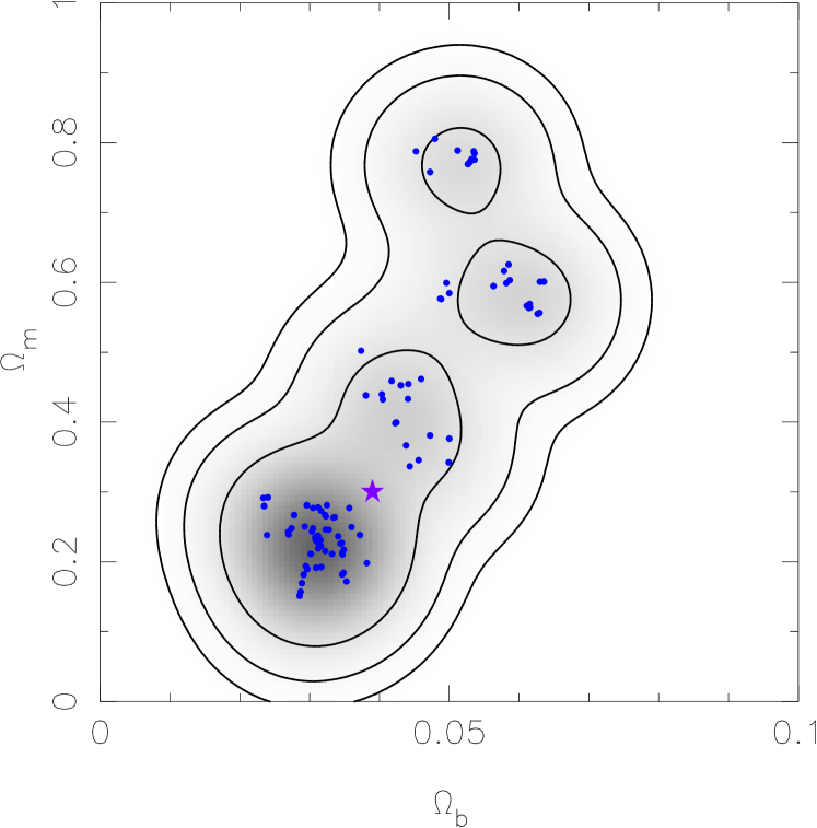
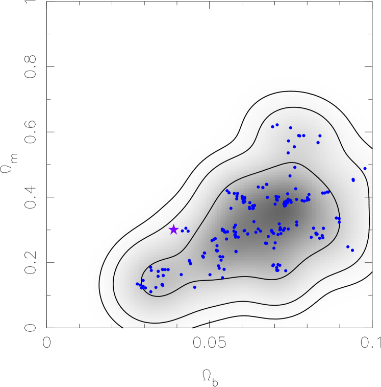
Figure 2: Cosmological parameters inferred for the two cluster models outlined in the text (Left, Model1; Right, Model2). The “true” values are marked with a star, contours represent 68, 95 and 99 percent confidence intervals. The samples used in generating the smooth distributions are shown as points.

5 Conclusions and Future Work

The Bayesian approach to cluster data analysis presented here is the natural extension of methods currently employed by observers: it provides an efficient way of exploring high-dimensional parameter spaces, a direct route from the experimental noise to uncertainties on the model parameters, and, in calculating the evidence, a way of discriminating between model-dependent statements.

We intend to include a larger array of cluster models of varying complexity, appropriate to the ever-improving data such as that expected from the next generation of SZ telescopes. X-ray data can also be included straightforwardly into the analysis, providing information on $H_{0}$ and the cluster temperature as well as improving the constraints on the other parameters.

References

References

- [1] M. Birkinshaw, Phys.Rep. 310, 97 (1999)
- [2] N. Kaiser and G. Squires, ApJ 404, 441 (1993)
- [3] P.J. Marshall et al. , submitted to MNRAS (2001), astro-ph/0112396
- [4] P.F. Scott et al. , in preparation
- [5] W.R. Gilks, S. Richardson, D.J. Spiegelhalter, “Markov-Chain Monte-Carlo In Practice”, Chapman and Hall (1996).
- [6] L. Grego et al. , ApJ 552, 2 (2001)
- [7] W.L. Freedman et al. , ApJ 553, 47 (2001)
- [8] S. Burles, K.M. Nollett, M.S. Turner, ApJ 552, L1 (2001)