Precise Measurements of Atmospheric Muon Fluxes with the BESS Spectrometer

Abstract

The vertical absolute fluxes of atmospheric muons and muon charge ratio have been measured precisely at different geomagnetic locations by using the BESS spectrometer. The observations had been performed at sea level (30 m above sea level) in Tsukuba, Japan, and at 360 m above sea level in Lynn Lake, Canada. The vertical cutoff rigidities in Tsukuba ($36.2^{\circ}N$,$140.1^{\circ}E$) and in Lynn Lake ($56.5^{\circ}N$,$101.0^{\circ}W$) are 11.4 GV and 0.4 GV, respectively. We have obtained vertical fluxes of positive and negative muons in a momentum range from 0.6 to 20 GeV/$c$ with systematic errors less than 3 % in both measurements. By comparing the data collected at two different geomagnetic latitudes, we have seen an effect of cutoff rigidity. The dependence on the atmospheric pressure and temperature, and the solar modulation effect have been also clearly observed. We also clearly observed the decrease of charge ratio of muons at low momentum side with at higher cutoff rigidity region.

, , , , , , , , , , , , , , , , , , , , , , , , , , , , , , , , , , , , , ,

1 Introduction

The evidence for atmospheric neutrino oscillation has been reported from the Super-Kamiokande collaboration by using high-statistics samples of muon neutrino events [1]. There are two major sources of systematic errors in evaluating the neutrino flux; the flux of primary cosmic-rays and the production cross sections of secondary mesons; pions and kaons [2, 3, 4]. Recently, the fluxes of primary cosmic-ray particles, mainly consisting of protons and helium nuclei, have been measured precisely by two independent and consistent observations [5, 6]. Although the details of interaction model itself is hard to be determined, the measurement of atmospheric muons plays crucial role in evaluating the flux of atmospheric neutrinos because muons and muon neutrinos are produced always in pairs as decay products of mesons and the kinematics of meson and muon decay is well known.

The muon flux at sea level has been measured by many groups. However, there are large discrepancies among those measurements much larger than the statistical error quoted in each publication. Therefore it is conceivable that the difference comes from systematic effects such as uncertainties in momentum determination, geometrical factor, exposure time, particle identification, trigger efficiency and normalization procedure.

We report here precise measurements of the absolute flux of atmospheric muons at sea level at Tsukuba ($36.2^{\circ}N$,$140.1^{\circ}E$), Japan and Lynn Lake ($56.5^{\circ}N$,$101.0^{\circ}W$), Canada by using the BESS spectrometer [7]. The data were collected in ’95 (at Tsukuba) and in ’97, ’98 and ’99 (at Lynn Lake). The cutoff rigidities are 11.4 GV (at Tsukuba) and 0.4 GV (at Lynn Lake).

2 Spectrometer Setup

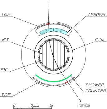
BESS ’99.

Figure 1: Cross-sectional view of the BESS ’95 and ’99 spectrometers.

The BESS spectrometer was designed as a high resolution spectrometer with a large geometrical acceptance to perform precise measurements of primary and secondary cosmic-rays as well as a sensitive search for rare exotic particles of primary origin[8, 9]. Cross sectional views of ’95 and ’99 configurations are shown in Fig. 1. The spectrometer configuration was updated in ’97 as described below, and was kept similar in ’98 and 99 except for shower counters installed in ’99.

The thin superconducting coil [10] (4.70 g/cm² thick including the cryostat) produces a uniform axial magnetic field of 1 Tesla. A jet-type drift chamber (JET), inner drift chambers (IDCs) and outer drift chambers (ODCs) are located inside and outside the coil. These chambers are operated with a slow gas (CO₂ 90 %, Ar 10 %). Tracking signal from the drift chambers are read out by flash ADCs. The $r\phi$-tracking is performed by fitting up to 28 hit-points, each with a spatial resolution of 200 $\mu$m. Tracking in the $z$-coordinate is made by fitting points in IDC measured with vernier pads with an accuracy of 470 $\mu$m and points in the JET chamber measured using charge-division with a spatial resolution of 20 mm. By using these data, we performed the continuous and redundant 3-dimensional track information. In order to get momentum of particle, we used 28 hit-points of the JET chamber and IDCs in the magnetic field. The ODCs provide extra hit positions outside the magnet and is used to calibrate the JET chamber and IDCs. In addition, all drift chambers have capabilities to distinguish the multi-hit. This feature enables us to recognize multi-track events, thus we could see the tracks having interactions and scatterings. The time-of-flight (TOF) scintillator hodoscopes measured the velocity of particles with a time resolution of 110 ps in ’95. The acrylic Čerenkov shower counter consists of acrylic and lead plate (12 mm). These counters are placed outside the lower TOF counter. The acrylic Čerenkov shower counters, used to separate electron and muons, were installed only for the ground observation. The total material thickness from outside the pressure vessel, passing through superconducting magnet coil, inside the JET chamber was 9.03 g/cm².

Since ’97 experiment, we installed a newly developed threshold-type Čerenkov counter with silica-aerogel radiator, after removing the ODCs [11]. The resolution of TOF was improved to 75 ps by using new photomultipliers (PMTs) with a larger diameter for better light collection [12]. In ’99 experiment, we installed a part of the shower counter just below the superconducting magnet.

3 Data Samples

The ’95 “ground” experiment was carried out at KEK, Tsukuba ($36.2^{\circ}N$,$140.1^{\circ}E$), Japan, from December 23 to 28. KEK is located at 30 m above sea level. The vertical cutoff rigidity is 11.4 GV [13]($\lambda=26.6^{\circ}N$ at geomagnetic latitude [14]). The mean atmospheric pressure in this experiment was 1010 hPa (1030 g/cm²). The scientific data were taken for a live time period of 291,430 sec and 9,148,104 events were recorded on magnetic tapes. The ’97, ’98 and ’99 ground experiments were carried out in Lynn Lake ($56.5^{\circ}N$, $101.0^{\circ}W$), Canada, on July 22, August 16 and July 26, respectively. The experimental site in Lynn Lake is located at 360 m above sea level. The vertical cutoff rigidity is 0.4 GV [13]($\lambda=65.5^{\circ}N$ at geomagnetic latitude [14]). The mean atmospheric pressures in Lynn Lake experiments in ’97, ’98 and ’99 were 980.6 hPa (1000 g/cm²), 990.5 hPa (1010 g/cm²) and 964.9 hPa (983.9 g/cm²), respectively. The total scientific data were obtained for a period of 21,304 sec (7,011 sec, 3,949 sec and 10,344 sec) of live time and 242,934, 137,629 and 354,869 events were recorded on the magnetic tapes, respectively.

The trigger was provided by a coincidence between the top and the bottom scintillators of TOF counters. All triggered events were gathered in the magnetic tapes. The core information (momentum, T.O.F., etc.) was composed and extracted from the original data. There were two kinds of efficiencies so as to gather atmospheric cosmic-ray data ; trigger efficiency ($\varepsilon_{trigger}$), track reconstruction efficiency ($\varepsilon_{reconstruction}$).

4 Data Analysis

At first, the following off-line selections were applied for the recorded events.

(i) One or two counters are hit in each layer of the TOF hodoscope and only one track should be found in the JET chamber.

(ii) Track should be fully contained in the fiducial region, namely the number of hits in the JET chamber expected from the trajectory should be 24 and the extrapolated track should cross the fiducial region of TOF scintillators ($|z|<43.0$ cm).

We call an efficiency that pass through these selection by the name of single track efficiency ($\varepsilon_{single}$). We used Monte Carlo calculation in order to obtain efficiency which depend on the momentum.

Next, we selected muon tracks from tracks that pass through the above selection. In order to select the muon tracks, we used the time-of-flight and rigidity information obtained by the TOF scintillation counters and drift chambers, respectively as shown in Fig. 2. We selected the muon tracks using ”muon $\beta^{-1}$-band cut” which are defined by :

$$\frac{1}{\beta}\>=\>\sqrt{\left(\frac{m}{R}\right)^{2}+1}\;\pm\;3.89\sigma.~{}~{}~{}(0.01\%)$$

Here, $\beta$ is velocity of particle, $m$ is muon mass and rigidity($R$) is momentum per charge. We selected particles which pass through this requirement ($<|3.89\sigma|$), and we call this selection efficiency muon selection efficiency ($\varepsilon_{\mu-select}$). From the plots, protons, electrons and positrons are major sources of background events that contaminates the muon bands.

The rejection of electrons and positrons was performed by utilizing the Acrylic Čerenkov shower counter. Proton events could be eliminated in a rigidity range below 1.4 GV by muon $\beta^{-1}$-band cut. Above this rigidity, we used other experimental data of proton flux [15, 16, 17] to reduce the contamination of protons into muon $\beta^{-1}$-band. A contamination of protons in the muon $\beta^{-1}$-band was estimated to be 2.0 % at 1.4 GV and decreased rapidly with rigidity. According to the work of R. L. Golden et al. [17], the proton flux at sea level follows the power spectrum with an index of about $-3.0$ from 2 to 20 GV, steeper than the index of muon flux on the ground level. The protons were subtracted from observed muon $\beta^{-1}$-band using the result of R. L. Golden et al. normalized to number of protons below 1.4 GV obtained in this experiment. A contamination of electrons and positrons in the muon $\beta^{-1}$-band cut was estimated by using Acrylic Čerenkov shower counter. The electrons interacts with lead plates (12 mm) and it generates shower in acrylic plates. Therefore Čerenkov light yielded by electrons are distinguished from that of muons [18]. A contamination was estimated to be about 2 % at 0.5 GV and decreased drastically with rigidity, because the electron flux had steeper index than that of the the muon index. We subtracted electrons and positrons from muon $\beta^{-1}$-band cut by using the estimation obtained by analysing the Acrylic Čerenkov shower counter. The systematic errors of these subtraction was 1 % for protons at 1.4 GeV/$c$ and 0.5 % for electrons and positrons at 0.6 GeV/$c$. The systematic errors decreased drastically as rigidity increases and it was negligible at 20 GeV/$c$. We used muon events that pass through only these selections to obtain muon energy spectrum. As we shall see later, we had about 98.9 % efficiency to take the muon events.

Based on these muon events, we obtained the muon rigidity spectrum at the top of instrument (TOI) in the following way: The TOI energy of each event was calculated by tracing back the particle through the spectrometer material and correcting energy loss by using GEANT 3.21. The corrections were usually small, about 10 MeV for a 1 GeV event.

Among the factors necessary to obtain the flux, the geometrical acceptance can be calculated reliably by Monte Carlo (M.C.) methods due to the simple geometry and the uniform magnetic field of the BESS spectrometer. The geometrical acceptance for the vertical muons ($\cos\theta\geq 0.98$) taken in Tsukuba (’95) was about 0.03 m²sr above 2 GeV/$c$ and decreased gradually at lower momentum. Because east and west effect is not important at high latitude, we analyze the data taken at Lynn Lake (’97, ’98 and ’99), in a range of $\cos\theta\geq 0.90$ (0.09 m²Sr). The systematic error caused by the east-west effect in Tsukuba was estimated to be 1.0 % by comparison with the experimental data and the isotropic M.C. calculation, and to be negligible in Lynn Lake. The mean value of zenith angle distribution of muon flux was $\cos\theta=0.990$ for Tsukuba data ($\cos\theta\geq 0.98$), and $\cos\theta=0.955$ for Lynn Lake data ($\cos\theta\geq 0.90$). We estimated that the total systematic error of the geometrical acceptance was 0.4 %. The geometrical acceptance can be calculated reliably both by an analytical method and by Monte Carlo methods at simple geometries, such as circle, quadrangle, etc. The difference of the results obtained by both methods was negligible (less than 0.2%). A systematic error of geometrical acceptance due to imperfect alignment was dominant. The livetime fraction of exposure time was 94.9 % (’95) and 99.3 % (’97, ’98 and ’99); the error due to this factor was negligibly small.

In summary, the efficiencies used in deriving the muon flux were trigger efficiency ($\varepsilon_{trigger}$), track reconstruction efficiency ($\varepsilon_{reconstruction}$), single track efficiency ($\varepsilon_{single}$) and muon selection efficiency ($\varepsilon_{\mu-select}$). The trigger was provided by a coincidence between the top and the bottom scintillators, with the threshold set at 1/3 of the pulse height from vertically incident minimum ionizing particles. $\varepsilon_{trigger}$ was obtained from pulse height distribution of the TOF counter. The efficiency for the trigger ($\varepsilon_{trigger}$) was estimated to be 99.95 %. All triggered events were recorded in magnetic tape, thereafter data summary tape (DST) was constructed by using the calibration data base. The DST contains information of the track (momentum, track length, etc.), therefore only reconstructed events were filled in DST and we analyzed the muon flux by using DST. In order to estimate $\varepsilon_{reconstruction}$, we made off-line scanning (eye scanning) for about 1000 tracks by using data made before DST and $\varepsilon_{reconstruction}$ was found to be 99.5 %. The single track selection efficiency ($\varepsilon_{single}$) was obtained from the M.C. simulation and the systematic error was estimated by examining agreements between observed and simulated distributions of the values used in the single track selection. $\varepsilon_{single}$ was found to be 99.5 %. The M.C. data agreed with the real data within 1.5 % in total. In order to select the muon events, we utilized the $\beta$ band cut that has a width of 3.89 $\sigma$, thus the muon selection efficiency ($\varepsilon_{\mu-select}$) was 99.99 %. From the efficiencies mentioned above, the total efficiency was found to be 98.9 %.

In order to eliminate possible influence of the momentum resolution to the muon flux, we used momentum up to 20 GeV/$c$. The momentum resolution of BESS spectrometer was $\Delta P/P=0.005P$ (M.D.M.$=200$ GeV/$c$). Therefore the errors of the muon flux was 1 % at 20 GeV/$c$ by M.C. calculation if we assumed the spectral index of muon flux is $-2.7$. Our previous paper [5] discussed about this spectrum deformation effect of the BESS spectrometer. As the momentum decreases, this error decreases. Then the errors caused by this effect was negligible at 0.6 GeV/$c$.

Summation of all the estimated systematic errors were 2.4 % for positive muons and 2.2 % for negative muons in Tsukuba and 2.2 % for positive muons and 1.9 % for negative muons in Lynn Lake.

5 Atmospheric Effect

Variations in cosmic-ray flux by the change of the atmospheric conditions is called ”atmospheric effect”. It has been known that there are two main sources of this effect [19] due to variations of the atmospheric pressure and temperature. Denoting integral flux of the muons at depth $x_{0}$ (g/cm²) as $I(\overline{E_{0}},x_{0},\theta)$, and the changes of atmospheric pressure and temperature as $\delta P$ (mb) and $\delta T(x)$ at $x$ (g/cm²) $(x<x_{0})$, we have a relation of

$$\delta I(\overline{E_{0}},x_{0},\theta)/I(\overline{E_{0}},x_{0},\theta)=-\beta(\overline{E_{0}},x_{0},\theta)\delta P+\int_{0}^{x_{0}}\alpha(x,\overline{E_{0}},x_{0},\theta)\delta T(x)dx,$$

Here, $E_{0}$ is the total energy of muons at $x_{0}$, $\overline{E_{0}}$ is the threshold energy, and $\beta(\overline{E_{0}},x_{0},\theta)$ and $\alpha(x,\overline{E_{0}},x_{0},\theta)$ are so called “barometric coefficient” and “partial temperature coefficient”, respectively.

In order to get the barometric coefficient, we used two sets of ’95 experimental data taken at different atmospheric pressures with a deviation of 25 hPa. Fig. 3 shows the barometric coefficient for the integral muon flux. The barometic effect has a negative correlation, and then flux decreases if the atmospheric pressure increases. A specific negative correlation due to the increases of the $\mu-e$ decay is expected dominant below 2 GeV/$c$ and another specific negative effect due to the absorption by the ionization loss becomes dominant above 2 GeV/$c$. The observed coefficient seemed to be consistent with calculated values as shown in Fig. 3. The effect at the 25 hPa pressure-difference on the muon flux amounts to be 2.5 % below 1 GeV/$c$ and less than 1 % above 5 GeV/$c$.

The temperature effect was calculated by using a temperature coefficient reported by S. Sagisaka [19], and observed variations in ’95 experimental data are shown in Fig. 4. We used high altitude temperature data observed by using a radio sonde data taken at Tateno Meteorological Observatory ($36.1^{\circ}N$, $140.1^{\circ}E$, 10 km south of KEK) [20]. In order to analyse the temperature effect, we used two data sets which were taken at different temperature at the ’95 experiment. The observed variation seemed to be consistent with the calculated variation. The variation of muon flux due to the temperature effect in the period of this experiment was less than 1 %.

6 Solar Modulation

Fig. 5 shows annual variation of the muon flux in Lynn Lake. In order to distinguish small difference of each variation, the ’97 and ’98 muon fluxes are divided by the ’99 muon flux, and the flux of each year were combined in a wide momentum region to reduce the statistical errors. It is clearly shown that the ’99 flux is lower than other fluxes. The ’99 experiment was performed at the lowest ambient pressure among other three measurements. Since the barometric effect has the negative correlation, the reduction of the flux in ’99 can not be explained by the barometric effect. We need to takes into account an effect of the solar modulation. The solar activity varies globally with the 11 year solar cycle and the solar minimum was ’96 - ’97 and the solar maximum happened between ’00 and ’01 according to observations of sunspot numbers [21]. However, this effect appears about one year later in neutron monitor data [22]. Not only the muon flux, but also muon charge ratios ($\mu^{+}/\mu^{-}$) decrease below 3.5 GV if the low energy primary proton flux decreases by the solar modulation. These charge ratios of ’97, ’98 and ’99 experiments in this energy region (0.58 - 3.44 GeV/$c$) were $1.258\pm 0.017$, $1.235\pm 0.022$ and $1.218\pm 0.014$. These decreases were consistent to decreases of the muon flux. The decrease of charge ratios and muon fluxes are caused by decreasing of primary proton flux, therefore the effect of solar modulation were observed. The BESS spectrometer observed variation of the primary proton flux due to the solar modulation effect at an altitude of 37 km (launched from Lynn Lake) from ’97 to ’00 [23]. These variation shows about 20 % decrease at 2 GeV/$c$ from ’97 to ’99 and the difference of these fluxes becomes much smaller at higher momentum. The mean energy of the primary proton responsible to muons of 0.5 GeV/$c$ at sea level is about 20 - 30 GeV, and then the degree of muon flux is much smaller than that of primary proton flux at the same energy.

These difference of muon flux were 3 % around 1 GeV/$c$. These differences were within statistic and systematic errors with small bins and it was important to obtain spectral shape with small statistic errors. Therefore ’97, ’98 and ’99 experimental data sets were combined to obtain the muon flux in Lynn Lake.

7 Results

Fig. 6 shows the resultant positive and negative muon fluxes, and Table. 1 and Table. 2 summarize those data with systematic and statistic errors. We have observed the vertical fluxes of the positive and negative muons in a momentum range from 0.6 to 20 GeV/$c$ with an estimated systematic error of 2.4 % for the positive muons and 2.2 % for the negative muons in Tsukuba, and 2.2 % for the positive muons and 1.9 % for the negative muons in Lynn Lake. The cutoff rigidity at Tsukuba is much higher than Lynn Lake. By comparing the data collected at two different geomagnetic latitudes, we have observed an effect of cutoff rigidity.

Fig. 7 shows the total (positive and negative) differential muon spectra at Tsukuba and Lynn Lake, together with previous measurements [24, 25, 26, 27, 28, 29, 30, 31, 32, 33]. Our data on the muon fluxes those which were multiplied by $p^{2}$ at sea level are shown in Fig. 8. From these figures, it is clearly seen that the muon flux measured in Tsukuba and in Lynn Lake were different in lower momentum ranged below 3.5 GeV/$c$, but were in good agreement in higher momentum beyond 3.5 GeV/$c$. This is because the cutoff rigidity for primary cosmic-rays does not affect in higher momentum.

Fig. 9 shows ratios of positive and negative muons together with the previous measurements [33, 34, 35, 36, 37], and the results are summarized in Table. 3 and in Table. 4. It was seen that the charge ratio obtained in Tsukuba decreased below 3.5 GeV/$c$ while the charge ratio obtained in Lynn Lake remained almost constant value even in this energy range. This difference comes from the influence of the geomagnetic cutoff rigidity. Because the low momentum muons must be generated by the higher momentum protons at Tsukuba. The muon charge ratio observed in Tsukuba had to include systematic errors of proton subtraction and east-west effect. On the other hand, the muon charge ratio observed in Lynn Lake had systematic errors due to only proton subtraction. The systematic error due to proton contamination was less than 2 %, therefore the muon charge ratio observed in Lynn Lake had very small systematic errors.

8 Discussion

The obtained momentum spectrum appeared to be good agreement with recent CAPRICE 94 [33] data using the instruments of magnetic spectrometer. These data agreed well within the systematic and statistic errors. But the results of previous experiments were about 20 % larger than these recent experimental data. Most of these previous experiments needed normalization point in order to determine absolute muon fluxes. Since the spectrum shape is similar enough among those experiments, systematic errors of the absolute fluxes are supposed to be the main cause of these difference of absolute fluxes. Therefore we performed our observations with a great care to evaluate the efficiencies to detect the muon tracks. We then have muon fluxes with much smaller systematic errors.

The atmospheric effect was clearly observed. Our result agreed well with the expectation of the analytical calculation[19]. The barometric coefficient had about $-0.1$ %/hPa at 1 GeV/$c$. A temperature effect had less influence on the muon flux in comparison with the barometric effect. Our observation of the temperature effect can also interpreted quantitatively with the expectation of an analytical calculation[19]. Therefore for a precise calculation of the atmospheric neutrino flux precisely, we could include these effect in an analytical way.

The solar modulation effects to the muon flux at the ground level was clearly observed in our experiments. Not only decreasing of the total flux, but also decreasing of the muon charge ratio has been observed. Decreasing of the muon flux should be due to decreasing of primary proton flux according to a temporal variation of the solar modulation. In the atmospheric neutrino flux calculation, it may be important to consider even small changes of the muon fluxes caused by the solar modulation.

9 Conclusion

The vertical absolute fluxes of atmospheric muons have been precisely measured with systematic errors of 2.4 % or smaller. We observed the geomagnetic effect by comparing the muon fluxes observed at Tsukuba, Japan and Lynn Lake, Canada. Muon charge ratios obtained at these two sites also showed the geomagnetic effect. The precise measurement of the muon flux at sea level is very important to understand cosmic-ray interactions inside the atmosphere and to decide fundamental parameters to study atmospheric neutrino oscillation.

BESS ’95.

Figure 2: Scatter plots of $\beta^{-1}$ vs. rigidity for positively and negatively charged particles. (’95).

Figure 3: Barometric coefficient.

Figure 4: Flux ratio due to temperature effect.

Figure 5: Annual variation of the muon flux.

Lynn Lake (’97, ’98 and ’99).

Tsukuba (’95).

Figure 6: BESS results for vertical differential momentum spectra of the positive and negative muons at sea level .

Figure 7: BESS results of vertical differential momentum spectrum of muons at sea level together with previous data.

Figure 8: The muon fluxes measured by BESS

Figure 9: BESS results of muon charge ratio at sea level together with previous data.

Table 1: Positive Muon Flux (Tsukuba ’95).

Tsukuba, Japan
Momentum	Mean	$\mu^{+}$
Range	Momentum	Differential flux	Statistical Error	Systematic Error
(GeV/$c$)	(GeV/$c$)	(m-2sr-1sec-1(GeV/c)-1)
0.576-0.621	0.598	1.386e+01	2.6e-01	2.7e-01
0.621-0.669	0.645	1.375e+01	2.4e-01	2.6e-01
0.669-0.720	0.695	1.310e+01	2.2e-01	2.5e-01
0.720-0.776	0.748	1.332e+01	2.1e-01	2.5e-01
0.776-0.836	0.806	1.287e+01	2.0e-01	2.5e-01
0.836-0.901	0.868	1.236e+01	1.8e-01	2.4e-01
0.901-0.970	0.936	1.223e+01	1.7e-01	2.3e-01
0.970-1.045	1.008	1.192e+01	1.6e-01	2.3e-01
1.045-1.126	1.086	1.137e+01	1.5e-01	2.2e-01
1.126-1.213	1.170	1.091e+01	1.4e-01	2.1e-01
1.213-1.307	1.260	1.055e+01	1.3e-01	2.0e-01
1.307-1.408	1.357	9.951e+00	1.2e-01	1.9e-01
1.408-1.517	1.463	9.390e+00	1.1e-01	2.0e-01
1.517-1.634	1.575	8.989e+00	1.1e-01	1.9e-01
1.634-1.760	1.697	8.613e+00	1.0e-01	1.8e-01
1.760-1.896	1.828	7.962e+00	9.1e-02	1.7e-01
1.896-2.043	1.969	7.519e+00	8.6e-02	1.6e-01
2.043-2.201	2.121	7.094e+00	8.0e-02	1.5e-01
2.201-2.371	2.285	6.543e+00	7.3e-02	1.4e-01
2.371-2.555	2.462	6.000e+00	6.8e-02	1.2e-01
2.555-2.752	2.653	5.596e+00	6.3e-02	1.2e-01
2.752-2.965	2.857	5.139e+00	5.8e-02	1.1e-01
2.965-3.194	3.078	4.622e+00	5.3e-02	9.5e-02
3.194-3.441	3.315	4.212e+00	4.9e-02	8.6e-02
3.441-3.707	3.573	3.742e+00	4.4e-02	7.6e-02
3.707-3.993	3.847	3.417e+00	4.0e-02	6.9e-02
3.993-4.302	4.145	3.089e+00	3.7e-02	6.3e-02

Table 1: Positive Muon Flux (Tsukuba ’95).

Tsukuba, Japan
Momentum	Mean	$\mu^{+}$
Range	Momentum	Differential flux	Statistical Error	Systematic Error
(GeV/$c$)	(GeV/$c$)	(m-2sr-1sec-1(GeV/c)-1)
4.302-4.635	4.465	2.719e+00	3.4e-02	5.5e-02
4.635-4.993	4.809	2.419e+00	3.0e-02	4.9e-02
4.993-5.379	5.182	2.060e+00	2.7e-02	4.2e-02
5.379-5.795	5.583	1.873e+00	2.5e-02	3.8e-02
5.795-6.243	6.016	1.628e+00	2.2e-02	3.3e-02
6.243-6.726	6.478	1.448e+00	2.0e-02	2.9e-02
6.726-7.246	6.983	1.248e+00	1.8e-02	2.5e-02
7.246-7.806	7.519	1.101e+00	1.6e-02	2.2e-02
7.806-8.409	8.099	8.934e-01	1.4e-02	1.8e-02
8.409-9.059	8.728	7.962e-01	1.3e-02	1.6e-02
9.059-9.760	9.399	6.731e-01	1.2e-02	1.4e-02
9.760-10.514	10.126	5.634e-01	1.0e-02	1.1e-02
10.514-11.327	10.907	4.923e-01	9.2e-03	1.0e-02
11.327-12.203	11.754	3.982e-01	7.9e-03	8.1e-03
12.203-13.146	12.652	3.521e-01	7.2e-03	7.2e-03
13.146-14.163	13.649	2.790e-01	6.1e-03	5.7e-03
14.163-15.258	14.693	2.465e-01	5.5e-03	5.1e-03
15.258-16.437	15.826	2.016e-01	4.8e-03	4.2e-03
16.437-17.708	17.054	1.752e-01	4.3e-03	3.6e-03
17.708-19.077	18.378	1.440e-01	3.8e-03	3.0e-03
19.077-20.552	19.791	1.227e-01	3.3e-03	2.6e-03

Table 1: Negative Muon Flux (Tsukuba ’95).

Tsukuba, Japan
Momentum	Mean	$\mu^{-}$
Range	Momentum	Differential flux	Statistical Error	Systematic Error
(GeV/$c$)	(GeV/$c$)	(m-2sr-1sec-1(GeV/c)-1)
0.576-0.621	0.598	1.245e+01	2.5e-01	2.4e-01
0.621-0.669	0.645	1.262e+01	2.3e-01	2.4e-01
0.669-0.720	0.695	1.215e+01	2.1e-01	2.3e-01
0.720-0.776	0.748	1.186e+01	2.0e-01	2.3e-01
0.776-0.836	0.806	1.149e+01	1.9e-01	2.2e-01
0.836-0.901	0.868	1.113e+01	1.7e-01	2.1e-01
0.901-0.970	0.936	1.086e+01	1.6e-01	2.1e-01
0.970-1.045	1.008	1.021e+01	1.5e-01	1.9e-01
1.045-1.126	1.086	1.012e+01	1.4e-01	1.9e-01
1.126-1.213	1.170	9.572e+00	1.3e-01	1.8e-01
1.213-1.307	1.260	8.920e+00	1.2e-01	1.7e-01
1.307-1.408	1.357	8.722e+00	1.1e-01	1.7e-01
1.408-1.517	1.463	8.039e+00	1.0e-01	1.5e-01
1.517-1.634	1.575	7.590e+00	9.8e-02	1.4e-01
1.634-1.760	1.697	7.317e+00	9.2e-02	1.4e-01
1.760-1.896	1.828	6.662e+00	8.4e-02	1.3e-01
1.896-2.043	1.969	6.234e+00	7.9e-02	1.2e-01
2.043-2.201	2.121	5.787e+00	7.2e-02	1.1e-01
2.201-2.371	2.285	5.421e+00	6.7e-02	1.0e-01
2.371-2.555	2.462	4.966e+00	6.2e-02	9.5e-02
2.555-2.752	2.653	4.510e+00	5.7e-02	8.6e-02
2.752-2.965	2.857	4.075e+00	5.2e-02	7.8e-02
2.965-3.194	3.078	3.757e+00	4.8e-02	7.2e-02
3.194-3.441	3.315	3.353e+00	4.4e-02	6.5e-02
3.441-3.707	3.573	3.041e+00	4.0e-02	5.9e-02
3.707-3.993	3.847	2.694e+00	3.6e-02	5.2e-02
3.993-4.302	4.145	2.393e+00	3.3e-02	4.6e-02

Table 1: Negative Muon Flux (Tsukuba ’95).

Tsukuba, Japan
Momentum	Mean	$\mu^{-}$
Range	Momentum	Differential flux	Statistical Error	Systematic Error
(GeV/$c$)	(GeV/$c$)	(m-2sr-1sec-1(GeV/c)-1)
4.302-4.635	4.465	2.090e+00	2.9e-02	4.1e-02
4.635-4.993	4.809	1.878e+00	2.7e-02	3.7e-02
4.993-5.379	5.182	1.649e+00	2.4e-02	3.2e-02
5.379-5.795	5.583	1.430e+00	2.2e-02	2.8e-02
5.795-6.243	6.016	1.270e+00	2.0e-02	2.5e-02
6.243-6.726	6.478	1.104e+00	1.8e-02	2.2e-02
6.726-7.246	6.983	9.449e-01	1.6e-02	1.9e-02
7.246-7.806	7.519	8.376e-01	1.4e-02	1.7e-02
7.806-8.409	8.099	6.926e-01	1.3e-02	1.4e-02
8.409-9.059	8.728	5.978e-01	1.1e-02	1.2e-02
9.059-9.760	9.399	5.188e-01	1.0e-02	1.0e-02
9.760-10.514	10.126	4.598e-01	9.2e-03	9.3e-03
10.514-11.327	10.907	3.713e-01	7.9e-03	7.5e-03
11.327-12.203	11.754	3.101e-01	7.0e-03	6.3e-03
12.203-13.146	12.652	2.625e-01	6.2e-03	5.4e-03
13.146-14.163	13.649	2.335e-01	5.6e-03	4.8e-03
14.163-15.258	14.693	1.958e-01	5.0e-03	4.0e-03
15.258-16.437	15.826	1.599e-01	4.3e-03	3.3e-03
16.437-17.708	17.054	1.320e-01	3.8e-03	2.7e-03
17.708-19.077	18.378	1.126e-01	3.4e-03	2.4e-03
19.077-20.552	19.791	9.271e-02	2.9e-03	1.9e-03

Table 2: Positive Muon Flux (Lynn Lake ’97,’98,’99).

Lynn Lake, Canada
Momentum	Mean	$\mu^{+}$
Range	Momentum	Differential flux	Statistical Error	Systematic Error
(GeV/$c$)	(GeV/$c$)	(m-2sr-1sec-1(GeV/c)-1)
0.576-0.669	0.622	1.620e+01	3.9e-01	2.6e-01
0.669-0.776	0.723	1.526e+01	3.4e-01	2.5e-01
0.776-0.901	0.839	1.494e+01	3.0e-01	2.4e-01
0.901-1.045	0.973	1.405e+01	2.6e-01	2.3e-01
1.045-1.213	1.128	1.280e+01	2.3e-01	2.1e-01
1.213-1.408	1.309	1.157e+01	2.0e-01	1.9e-01
1.408-1.634	1.519	1.047e+01	1.7e-01	2.0e-01
1.634-1.896	1.763	8.831e+00	1.5e-01	1.6e-01
1.896-2.201	2.046	7.744e+00	1.3e-01	1.4e-01
2.201-2.555	2.373	6.844e+00	1.1e-01	1.2e-01
2.555-2.965	2.752	5.354e+00	9.0e-02	9.6e-02
2.965-3.441	3.194	4.541e+00	7.7e-02	8.1e-02
3.441-3.993	3.705	3.640e+00	6.4e-02	6.4e-02
3.993-4.635	4.299	2.928e+00	5.3e-02	5.2e-02
4.635-5.379	4.991	2.190e+00	4.3e-02	3.8e-02
5.379-6.243	5.795	1.789e+00	3.6e-02	3.1e-02
6.243-7.246	6.718	1.340e+00	2.9e-02	2.3e-02
7.246-8.409	7.790	1.017e+00	2.3e-02	1.8e-02
8.409-9.760	9.046	7.332e-01	1.8e-02	1.3e-02
9.760-11.327	10.504	5.437e-01	1.5e-02	9.6e-03
11.327-13.146	12.172	3.784e-01	1.1e-02	6.8e-03
13.146-15.258	14.144	2.838e-01	9.1e-03	5.1e-03
15.258-17.708	16.385	1.924e-01	7.0e-03	3.5e-03
17.708-20.552	19.078	1.436e-01	5.6e-03	2.6e-03

Table 2: Negative Muon Flux (Lynn Lake ’97,’98,’99).

Lynn Lake, Canada
Momentum	Mean	$\mu^{-}$
Range	Momentum	Differential flux	Statistical Error	Systematic Error
(GeV/$c$)	(GeV/$c$)	(m-2sr-1sec-1(GeV/c)-1)
0.576-0.669	0.622	1.327e+01	3.4e-01	2.2e-01
0.669-0.776	0.723	1.307e+01	3.0e-01	2.1e-01
0.776-0.901	0.839	1.189e+01	2.6e-01	1.9e-01
0.901-1.045	0.973	1.129e+01	2.3e-01	1.8e-01
1.045-1.213	1.128	1.041e+01	2.1e-01	1.7e-01
1.213-1.408	1.309	9.649e+00	1.8e-01	1.6e-01
1.408-1.634	1.519	8.295e+00	1.5e-01	1.3e-01
1.634-1.896	1.763	7.229e+00	1.3e-01	1.2e-01
1.896-2.201	2.046	6.456e+00	1.2e-01	1.0e-01
2.201-2.555	2.373	5.256e+00	9.6e-02	8.6e-02
2.555-2.965	2.752	4.368e+00	8.1e-02	7.1e-02
2.965-3.441	3.194	3.506e+00	6.7e-02	5.8e-02
3.441-3.993	3.705	2.861e+00	5.7e-02	4.7e-02
3.993-4.635	4.299	2.281e+00	4.7e-02	3.8e-02
4.635-5.379	4.991	1.735e+00	3.8e-02	2.9e-02
5.379-6.243	5.795	1.369e+00	3.1e-02	2.3e-02
6.243-7.246	6.718	9.978e-01	2.5e-02	1.7e-02
7.246-8.409	7.790	7.590e-01	2.0e-02	1.3e-02
8.409-9.760	9.046	5.605e-01	1.6e-02	9.7e-03
9.760-11.327	10.504	4.000e-01	1.3e-02	7.0e-03
11.327-13.146	12.172	2.900e-01	9.9e-03	5.1e-03
13.146-15.258	14.144	2.130e-01	7.9e-03	3.8e-03
15.258-17.708	16.385	1.381e-01	5.9e-03	2.5e-03
17.708-20.552	19.078	9.773e-02	4.6e-03	1.8e-03

Table 3: Muon Charge Ratio (Tsukuba ’95).

Tsukuba, Japan
Momentum	Mean
Range	Momentum	$\mu^{+}/\mu^{-}$ Ratio	Statistical Error	Systematic Error
(GeV/c)	(GeV/c)
0.576-0.669	0.623	1.100	0.020	0.011
0.669-0.776	0.723	1.101	0.018	0.011
0.776-0.901	0.838	1.115	0.017	0.011
0.901-1.045	0.973	1.147	0.016	0.011
1.045-1.213	1.129	1.132	0.015	0.011
1.213-1.408	1.309	1.161	0.015	0.012
1.408-1.634	1.520	1.177	0.015	0.016
1.634-1.896	1.762	1.186	0.014	0.016
1.896-2.201	2.045	1.216	0.015	0.016
2.201-2.555	2.373	1.208	0.014	0.015
2.555-2.965	2.754	1.251	0.015	0.016
2.965-3.441	3.195	1.243	0.015	0.015
3.441-3.993	3.708	1.249	0.016	0.015
3.993-4.635	4.302	1.296	0.017	0.015
4.635-5.379	4.991	1.269	0.017	0.014
5.379-6.243	5.793	1.296	0.019	0.014
6.243-7.246	6.725	1.316	0.020	0.014
7.246-8.409	7.801	1.303	0.022	0.014
8.409-9.760	9.048	1.315	0.024	0.014
9.760-11.327	10.499	1.272	0.025	0.013
11.327-13.146	12.177	1.312	0.028	0.013
13.146-15.258	14.146	1.225	0.029	0.012
15.258-17.708	16.408	1.292	0.034	0.013
17.708-20.552	19.044	1.299	0.037	0.013

Table 4: Muon Charge Ratio (Lynn Lake ’97,’98,’99).

Lynn Lake, Canada
Momentum	Mean
Range	Momentum	$\mu^{+}/\mu^{-}$ Ratio	Statistical Error	Systematic Error
(GeV/c)	(GeV/c)
0.576-0.901	0.739	1.217	0.023	0.000
0.901-1.408	1.147	1.223	0.019	0.000
1.408-2.201	1.781	1.226	0.017	0.011
2.201-3.441	2.761	1.274	0.018	0.009
3.441-5.379	4.288	1.273	0.020	0.007
5.379-8.409	6.676	1.328	0.025	0.005
8.409-13.146	10.382	1.325	0.032	0.003
13.146-20.552	16.170	1.388	0.044	0.001

References

- [1] Y. Fukuda et al., Phys. Rev. Lett. 81 (1998) 1562.
- [2] T. K. Gaisser et al., Phys. Rev. D 54 (1996) 5578.
- [3] T. K. Gaisser and M. Honda, Preprint, hep-ph/0203272.
- [4] M. Honda et al., Phys. Rev. D 52 (1995) 4985 .
- [5] T. Sanuki et al., Ap. J. 545 (2000) 1135.
- [6] J. Alcaraz et al., Phys. Lett. B 472 (2000) 215.
- [7] Y. Ajima et al., Nucl. Instr. and Meth. A, 443 (2000) 71.
- [8] S. Orito, KEK Report 87-19, Proceedings of the ASTROMAG Workshop, edited by J. Nishimura, K. Nakamura, A. Yamamoto. (1987) p.111.
- [9] A. Yamamoto et al., Adv. Space Res., 14 (1994) 75.
- [10] A. Yamamoto et al., IEEE Trans. Magn. 24 (1988) 1421.
- [11] Y. Asaoka et al., Nucl. Instr. and Meth. A, 416 (1998) 236.
- [12] Y. Shikaze et al., Nucl. Instr. and Meth. A, 455 (2000) 596.
- [13] M. A. Shea et al., Proc. 27th ICRC 2001(Hamburg), (2001) 4063.
-
[14]
World Data Center for Geomagnetism, Kyoto University,
Ψhttp://swdcdb.kugi.kyoto-u.ac.jp/trans/index.html
- [15] G. Brooke and A. W. Wolfendale, Proc. Phys. Soc. 83 (1964) 843.
- [16] I. S. Diggory et al., J. Phys. A:Math.,Nucl. Gen., 7 (1974) 741.
- [17] R. L. Golden et al., J. Geophys. Res., 100 (1995) 23,515.
- [18] T. Sanuki, KEK Proceedings 94-11 (1995) 53.
- [19] S. Sagisaka, IL NUOVO CIMENT 9C (1986) 809.
- [20] Aerological Data of Japan, edited by Japan Meteorological Agency (monthly issued).
-
[21]
NASA/Marshall Space Flight Center,
Ψhttp://wwwssl.msfc.nasa.gov/ssl/pad/solar/sunspots.htm
-
[22]
University of Chicago, Neutron Monitor Datasets,
Ψhttp://ulysses.uchicago.edu/NeutronMonitor/neutron_mon.html
- [23] Y. Asaoka et al., Phys. Rev. Lett. 88 (2002) 051101-1.
- [24] P. J. Hayman et al., Proc. Phys. Soc. London. 80 (1962) 710.
- [25] P. J. Green et al., Phys. Rev. D 20 (1979) 1598.
- [26] C. A. Ayre et al., J. Phys. G 1 (1975) 584.
- [27] B. C. Nandi et al., J. Phys. A 5 (1972) 1384.
- [28] O. C. Allkofer et al., Phys. Lett. B 36 (1971) 425.
- [29] B. J. Bateman et al., Phys. Lett. B 36 (1971) 144.
- [30] B. C. Rastin, J. Phys. G 10 (1984) 1609.
- [31] S. Tsuji et al., J. Phys. G: Nucl. Part. Phys. 24 (1998) 1805.
- [32] M. P. DePascale et al., J. Geophysical Res. 98 (1993) 3501.
- [33] J. Kremer et al., Phys. Rev. Lett. 83 (1999) 4241.
- [34] I. C. Appleton et al., Nucl. Phys. B 26 (1971) 365.
- [35] J. M. Baxendale et al., J. Phys. G 7 (1975) 781.
- [36] B. C. Nandi et al., Nucl. Phys. B 40 (1972) 289.
- [37] B. C. Rastin, J. Phys. G 10 (1984) 1629.