AGN-selected clusters as revealed by weak lensing

Abstract

As a pilot study to investigate the distribution of matter in the fields of powerful AGN, we present weak lensing observations of deep fields centered on the radio-quiet quasar E1821$+$643, the radio galaxy 3C 295, and the two radio-loud quasars, 3C 334 and 3C 254. The host clusters of E1821$+$643 and 3C 295 are comfortably detected via their weak lensing signal, and we report the detection of a cluster-sized mass concentration in the field of the $z=0.734$ quasar 3C 254. The data for the 3C 334 field are so far inconclusive. We find that the clusters are massive and have smooth mass distributions, although one shows some evidence of past merger activity. The mass-to-light ratios are found to be moderately high. We discuss the results in light of the cooling flow and the merger/interaction scenarios for triggering and fuelling AGN in clusters, but find that the data do not point unambiguously to neither of the two. Instead, we speculate that sub-cluster mergers may be responsible for generating close encounters or mergers of galaxies with the central cluster member, which could trigger the AGN.

1 Introduction

The causes of the dramatic cosmic evolution of AGN (e.g. Dunlop & Peacock 1990; Hartwick & Schade 1990) remain unclear, we have little knowledge of how and why AGN form, how quasar activity is triggered and sustained in a galaxy, and what extinguishes the activity. The findings that AGN are often associated with other galaxies is believed to indicate that interactions between galaxies may play a role, since interactions are more likely to occur in a dense environment. Host galaxies and their close companions have been found to display disturbed morphology (e.g. Bahcall et al. 1997; Canalizo & Stockton 2001), also taken as a sign that interactions have taken place. Even in cases where companion galaxies appear undisturbed in the optical, radio images taken at redshifted 21cm (of nearby AGN) show long bridges or tidal tails of HI gas connecting the AGN with a close neighbour [Lim & Ho 1999].

These observations have raised the question of the existence and the nature of a physical link between the AGN and its environment. Two very different scenarios for this link have been suggested, the merger/interaction and the cooling flow scenario.

Ellingson, Green & Yee [Ellingson et al. 1991a] found evidence for the merger/interaction scenario when they made multi-object spectroscopy of galaxies associated with optically luminous quasars. They found that the richest quasar host clusters have abnormally low velocity dispersions compared to those of clusters in general with similar optical richness. This is consistent with the idea that galaxy-galaxy interactions are related to the quasar phenomenon, (e.g. Hutchings, Crampton & Campbell 1984), since in dynamically young clusters where the galaxies have low velocities, the encounters between galaxies will be disruptive and perhaps trigger or fuel quasar activity in one of the interacting galaxies.

Further support for this was found by Yee & Green [Yee & Green 1987] and Ellingson et al. [Ellingson et al. 1991b] in their studies of quasar environments. Optically luminous quasars were found more frequently in rich environments at $z\ga 0.6$ than at lower redshifts, suggesting that by $z\sim 0.3$–0.4, the quasars in rich clusters have faded. Since the time elapsed between $z\sim 0.4$ and $z\sim 0.6$ corresponds to the dynamical time scales of cluster cores, they proposed that dynamical changes in the cluster environments were responsible for the fading of quasars, perhaps as a result of lack of gaseous fuel after the clusters virialize. Accordingly, highly luminous AGN should therefore not exist in rich clusters at low redshifts, but there are several examples which contradict this, demonstrating that the requirement of non-virialized clusters is not sufficient. One example is Cygnus A, a powerful FRII radio galaxy in a rich cluster at $z=0.056$. Two other examples, which we study in this paper, are 3C 295 and E1821$+$643. 3C 295 is a powerful FRII radio galaxy in a cluster at $z=0.46$, and E1821$+$643 is an optically luminous quasar at $z=0.297$ situated in a very rich cluster.

The cooling flow scenario has been discussed by e.g. Fabian et al. [Fabian et al. 1986], Fabian & Crawford [Fabian & Crawford 1990] and Bremer, Fabian & Crawford [Bremer, Fabian & Crawford 1997]. In this picture, cooling flows in sub-clusters at earlier epochs provide fuel for the AGN, but as sub-clusters merge toward the present epoch, the cooling flows are disrupted and the quasar activity switched off. Alternatively, the quasar may switch off when the cooling flow gas is exhausted [Fabian & Crawford 1990]. Several observations have been made of extended emission-line gas around powerful quasars which seem to support the cooling flow model (e.g. Crawford & Fabian 1989; Forbes et al. 1990; Bremer et al. 1992).

However, it is not established yet whether extended emission line gas indicates the presence of a cooling flow. For instance, the emission lines could be produced by radio source shocks instead of gas cooling out of the flow (e.g. Tadhunter et al. 2000). The standard cooling flow model (Fabian 1994 and references therein) has received some criticism lately since XMM observations of cooling flow clusters do not show emission lines at temperatures below 1 keV as predicted (Peterson et al. 2001; Tamura et al. 2001; Kaastra et al. 2001). This suggests that the cooling flow model may need to be re-evaluated, and in many cases mass deposition rates may turn out to be lower than originally thought. Heating by AGN has been proposed as a possible cause of the apparent lack of cold gas, but new Chandra data seem to indicate that the coolest gas is close to the radio lobes, contrary to what is expected if there is heating by the AGN (Fabian 2001).

If cooling flows were the chief mechanism for providing fuel to the most powerful AGN in clusters, we should observe more rich clusters with central, powerful AGN than we do. In fact, most rich AGN host clusters do not contain anything more powerful than an FRI source (like M87 in the Virgo cluster). In a sample of 260 rich-cluster radio galaxies studied by Ledlow, Owen & Eilek [Ledlow et al. 2002], there are almost no FRII radio galaxies with luminosities at 1.4 GHz greater than $10^{25.5}$ W Hz^-1.

Hall et al. [Hall et al. 1995] and Hall, Ellingson & Green [Hall et al. 1997] used X-ray data from ROSAT and Einstein to derive physical parameters, such as gas density and temperature, of AGN host clusters. Their aim was to distinguish between three different models for the evolution of AGN in clusters, the young cluster scenario, the cooling flow model, and a model of decreasing ICM density with increasing redshift (Stocke & Perrenod 1981). Three of the five clusters in their sample were not detected, but upper limits on their X-ray luminosity could be estimated. They found that neither a cooling flow nor a decrease in ICM density could explain all their observations, and proposed that strong interactions between the AGN host and another galaxy in the cluster could be the only necessary mechanism to produce powerful AGN in clusters.

In this paper, we investigate the link between four powerful AGN and their environments by using weak lensing methods. The weak lensing technique allows us to probe the distribution of total mass (dark + luminous) in the AGN fields, and the mass distributions can be used to test the merger/interaction and the cooling flow scenarios. The two scenarios make very different predictions about the dynamical state of AGN host clusters, and by investigating the cluster dynamics, it may be possible to find which, if any, of these two mechanisms are responsible for the AGN–environment link.

A cooling flow is expected to be associated with a single deep potential well in an evolved, virialized cluster [Edge et al. 1992], and in this case we expect a strong weak lensing signal and a mass distribution characterized by only a single peak. In contrast, if the AGN activity is related to galaxy interactions, these will be much more disruptive if the encounter velocities are relatively low and comparable to the internal velocity dispersions of the galaxies involved. Consequently, a cluster that is still forming will be preferred, as in such a cluster there is an increased probability for low-velocity encounters. A dynamically young cluster is expected to have an irregular mass distribution, possibly with several sub-clumps [Schindler 2001].

Our method of cluster selection is based on the detection of weak gravitational shear and the presence of an AGN. This is different from the usual methods of detecting clusters, by optical richness or X-ray luminosity. Whereas optical and X-ray cluster surveys are biased toward the most baryon-rich systems, clusters selected by their weak shear signal are biased toward the most massive systems in terms of dark+luminous mass. If there is a large range in the baryonic-to-dark matter ratio in clusters, clusters with high mass-to-light (hereafter M/L) ratios will have been missed in optical and X-ray surveys. Although we present a case-by-case study here, it is nevertheless interesting to compare the masses and the M/L ratios of the AGN host clusters to those of clusters detected on the basis of optical richness or X-ray luminosity.

The outline of the paper is as follows. In Section 2 we describe the selection of the targets and review some of their properties. Section 3 describes the observations and the data reduction. Before the weak lensing analysis is performed, we investigate the colour-magnitude diagrams of the clusters in Section 4. The purpose of this is to locate the colour-magnitude relation in the known clusters, E1821$+$643 and 3C 295, and thereby identify cluster galaxies that do not contribute to the weak lensing signal. We also investigate the colour-magnitude diagram of 3C 254 and discuss whether there is evidence for a red sequence of early-type cluster galaxies in this field. A brief introduction to the weak lensing method and how we measure the gravitational shear is given in Section 5. We follow the standard approach for ground-based data and use the Kaiser, Squires & Broadhurst [Kaiser et al. 1995] formalism to correct for PSF anisotropies using the imcat software, and the approach by Luppino & Kaiser [Luppino & Kaiser 1997] to calibrate galaxy ellipticities to gravitational shear. In Section 6, we present the results of the analysis by showing maps of the projected surface mass density in the fields, plots of the shear profiles in the clusters, and estimates of masses and M/L ratios. The results are discussed in Section 7, and conclusions are drawn in Section 8.

Our assumed cosmology has $h=H_{0}/100$ km s^-1 Mpc^-1, $\Omega_{0}=1$ and $\Omega_{\Lambda}=0$ .

2 The sample

We selected four powerful AGN with extended X-ray emission for this study. Two of the targets are well-known cases of an AGN associated with a galaxy cluster, the radio galaxy 3C 295 and the radio-quiet quasar E1821$+$643. The other two targets are the radio-loud quasars 3C 334 and 3C 254 which were found to have significant extended X-ray emission in moderately deep ROSAT pointings (Hardcastle & Worrall 1999; Crawford et al. 1999). For the former two sources, we know that the extended X-ray emission originates in the hot intra-cluster medium of the host clusters, but in the latter two cases no host clusters are known. Their extended X-ray emission is however an indicator of clustered galaxy environments provided that the point-like X-ray emission from the AGN has been properly subtracted, and that the extended component does not originate in processes associated with the AGN itself.

2.1 3C 295

This is a powerful FRII radio galaxy at $z=0.46$ with compact radio structure. In the optical, the radio galaxy is classified as a cD, and its host cluster has been extensively studied both at optical (Mathieu & Spinrad 1981; Dressler et al. 1997; Smail et al. 1997a,b; Standford, Eisenhardt & Dickinson 1998; Thimm et al. 1998) and X-ray wavelengths (Henry & Henriksen 1986; Mushotzky & Scharf 1997; Neumann 1999; Allen et al. 2001). It is not a particularly optically-rich cluster, most likely of Abell class 1 (Mathieu & Spinrad 1981; Hill & Lilly 1991), but its velocity dispersion is high, $\sim 1630$ km s^-1 [Dressler et al. 1999].

In X-rays, it appears to be a dynamically evolved and relaxed cluster with a high bolometric luminosity of $L_{\rm X}\approx 6.5\times 10^{44}h^{-2}$ [Neumann 1999]. It was suggested by Henry & Henriksen [Henry & Hendriksen 1986] that the cluster hosts a cooling flow, later confirmed by Neumann [Neumann 1999]. Allen et al. [Allen et al. 2001] have studied the cluster with the Chandra X-ray satellite and find that the cooling flow is 2–4$h$ Gyr old, with a mass deposition rate of 70$h^{-2}$ M_⊙ yr^-1.

3C 295 was one of the first two clusters in which a weak gravitational lensing signal was detected [Tyson, Valdes & Wenk 1990], and Smail et al. [Smail et al. 1997a] have performed weak lensing analysis on this field using HST WFPC2 data. The cluster displays signs of strong lensing and a quadruple lens has also been found (Fisher, Schade & Barrientos 1998; Lubin et al. 2000). Since this cluster is well-studied, it serves as a consistency check on our techniques.

Table 1: Data obtained during the three observing runs from 1998 to 2000. We list the seeing and the completeness limit in the combined images, but for 3C 295 and E1821$+$643, only using the combined $I$-band images from 1999, since these were used for the weak lensing analysis. The completeness limits are based on the turn-over in the number counts (from object detection with a 4$\sigma$ detection threshold).

Field	$z$	Filter	Exposure time (s)			Seeing	Completeness
			1998	1999	2000	(arcsec)	limit
E1821$+$643	0.297	$I$	7500	10800	–	0.83	24.5
		$V$	1800	7200	–	1.00	25.5
		$B$	–	15600	–	0.85	26.5
3C 295	0.460	$I$	9300	10800	–	0.76	25.0
		$V$	–	10800	–	0.95	25.5
3C 334	0.555	$I$	–	–	13790	0.62	23.5
3C 254	0.734	$I$	–	–	21747	0.50	24.0
		$V$	–	–	15500	1.10	26.5

2.2 E1821$+$643

This is an optically luminous quasar at $z=0.297$ residing in a giant elliptical host galaxy (Hutchings & Neff 1991; McLeod & McLeod 2001) at the centre of a very rich Abell class $\ga 2$ cluster (Schneider et al. 1992; Lacy, Rawlings & Hill 1992). The quasar is detected at radio wavelengths, has a compact core, a one-sided jet, and a radio luminosity of $L_{\rm 5GHz}\approx 1.2\times 10^{23}h^{-2}$ W Hz^-1 sr^-1 (Lacy et al. 1992; Blundell et al. 1996), but is classified as radio-quiet because of its high optical luminosity, $M_{B}\approx-27$.

The surrounding cluster was first noted in the optical by Hutchings & Neff [Hutchings & Neff 1991] who believed it was background to the quasar, but Schneider et al. [Schneider et al. 1992] took spectra of eight galaxies in the field, and found that six of them belonged to a cluster at the quasar redshift. Subsequently, spectra of several galaxies in this field have been obtained in studies of Ly$\alpha$ absorption systems (Le Brun et al. 1996; Tripp et al. 1998), and using published spectroscopic redshifts of 42 galaxies the cluster velocity dispersion is estimated to 1182$\pm$19 km s^-1 (kindly provided to us by B. Holden, using the biweight algorithm of Beers, Flynn & Gebhardt [Beers, Flynn & Gebhardt 1990] and a jackknife technique to estimate errors).

Even though it is one of the most X-ray luminous clusters known, with a bolometric luminosity of $L_{\rm X}\sim 10^{45}h^{-2}$ erg s^-1 [Saxton et al. 1997], it went undetected in X-rays for a long time due to the presence of the dominant quasar point source. But recently, Saxton et al. [Saxton et al. 1997] and Hall et al. [Hall et al. 1997] reported detections of excess X-ray emission around the quasar in ROSAT data. The X-ray data gave no firm evidence for a cooling flow, and observations made by Fried [Fried 1998] of extended emission-line gas around the quasar suggest that no cooling flow is present since the [oiii]/[oii] emission-line ratio does not increase outward as expected in a cooling flow.

It has been pointed out that this quasar has many of the properties typical of radio-loud quasars. It has a giant elliptical host, lies in a rich cluster, and the [oiii] luminosity in the extended emission-line region is more typical of that found in radio-loud quasars (Fried 1998, and references therein). However, E1821$+$643 fits well in with quasars from the FIRST Bright Quasar Survey (FBQS, Gregg et al. 1996; White et al. 2000) in the radio luminosity–optical luminosity plane. Lacy et al. [Lacy et al. 2001] used the FBQS to show that there is a continuous variation of radio luminosity with black hole mass for quasars. Using the H$\beta$ line width of E1821$+$643 [Kolman et al. 1993], an estimate of the black hole mass can be made (Kaspi et al. 1999), and we find that the black hole in E1821$+$643 has a mass of $\sim 1\times 10^{9}h^{-1}$ M_⊙ (for details, see Lacy et al. 2001). With this black hole mass and its radio luminosity, it fits very well the radio-luminosity – black hole mass relation of Lacy et al. and is therefore similar to the FBQS objects. E1821$+$643 might not be such a special case after all, and is probably typical of highly luminous radio-quiet quasars.

2.3 3C 334 and 3C 254

These are two powerful steep-spectrum radio-loud quasars at $z=0.555$ and $z=0.734$, respectively, and are the most distant quasars in our study. They were included in the sample because there exists evidence that they are surrounded by extended X-ray emission. At rest frame 0.1–2.0 keV, Crawford et al. [Crawford et al. 1999] find X-ray luminosities of 0.8–2.0$\times$10${}^{44}h^{-2}$ and 1.3–2.3$\times$10${}^{44}h^{-2}$ erg s^-1 for the emission around 3C 334 and 3C 254, respectively. If the extended emission is interpreted as thermal emission from a hot intra-cluster medium, the quasars may lie in rich clusters since the typical luminosity of Abell class 1 clusters is a few times $10^{44}h^{-2}$ erg s^-1 [Briel & Henry 1993].

There is further circumstantial evidence that 3C 334 and 3C 254 are associated with galaxy clusters. Optical images reveal an apparent overdensity of galaxies around 3C 254 [Bremer 1997], and Hintzen [Hintzen 1984] find a number of nearby companion galaxies to 3C 334, although Yee & Green [Yee & Green 1987] do not find any significant clustering in this field. Further suggestions that 3C 334 and 3C 254 lie in clusters come from observations of extended oxygen line-emission around the quasars where the pressures inferred from the oxygen lines are comparable to pressures in the intra-cluster medium of nearby clusters (Crawford & Fabian 1989; Forbes et al. 1990; Crawford & Vanderriest 1997). It is argued by Forbes et al. and Crawford & Vanderriest that 3C 254 might be embedded in a very massive cooling flow with a mass deposition rate of up to $250h^{-2}$ M_⊙ yr^-1 within 20$h^{-1}$ kpc of the quasar. If the quasar is indeed associated with a massive cooling flow, one might expect that the cluster around 3C 254 be very massive as well.

3 Observations and data reduction

Imaging observations were made with the 2.56-m Nordic Optical Telescope (NOT) using the ALFOSC (Andalucia Faint Object Spectrograph and Camera) instrument equipped with a 2k$\times$2k Loral CCD with pixel scale 0.189 arcsec, resulting in a 6.5$\times$6.5 arcmin² FOV. The NOT/ALFOSC is a well-suited instrument for weak lensing studies of clusters, both because the field of view is relatively large, and because the NOT site has excellent seeing conditions. A wide field of view ensures a large number of faint background galaxies to measure ellipticities on, thereby improving the statistics, and good seeing conditions minimize the noise in the determination of galaxy ellipticities.

Since the seeing is improved at longer wavelengths, we used the $I$-band images for measuring galaxy shapes. We therefore dedicated the time when the FWHM seeing was $\la 0.8$ arcsec to $I$-band imaging, and observed in $V$-band when the seeing increased to 0.9 arcsec. The E1821$+$643 cluster was also observed in the $B$-band since there is a planetary nebula in this field (K1-16, 88 arcsec NW of the quasar) which is relatively bright in $V$, but less bright in $B$, since most of the emission comes from [oiii]$\lambda\lambda$4959,5007.

The integrations were divided into exposures of 600 s each in the $B$- and $V$-band, and 300 or 450 s in the $I$-band, offsetting the telescope 10–15 arcsec between each exposure to avoid bad pixels falling consistently on the same spot.

We had in total three observing runs to obtain the data for this project, as summarized in Table 1. On the 1998 run, there were clouds and cirrus on several of the nights, and the conditions were therefore generally poor for doing weak lensing observations. A backup programme was done instead, but occasionally during clear periods, we could return to the weak lensing programme. During the 1999 and 2000 runs, the weather was clear and the conditions photometric.

The data reduction was performed using standard iraf routines for bias subtraction and flatfielding. For the flatfielding, we used twilight flats, but we also flatfielded the $I$-band data with a skyflat formed by taking the median of nine object frames. By dividing with the skyflat we were able to remove a fringing pattern before the images were combined. The fringing pattern is additive and should ideally be subtracted from the images, but we found that division with the skyflat removed the fringes much better. For 10 per cent fringes, the error in the photometry will be $\pm 0.1$ mag, but since our analysis is more critical to measuring galaxy shapes accurately, we chose a flat background level at the expense of accurate photometry.

After bias subtraction, flatfielding and fringe removal, the images were aligned and coadded using the iraf tasks imalign and combine with combine operation set to average. In order not to confuse the detection algorithm in the imcat software, we also flattened out large-scale variations in the sky level by subtracting off a model of low-frequency variations in the background level.

The photometric zero points were determined by taking images of standard star fields [Landolt 1992], and the atmospheric extinction was estimated by observing the standard fields at different airmasses. Galactic reddening was corrected for by looking up the amount of extinction in the NED. The NED values are based on reddening maps by Schlegel, Finkbeiner & Davis [Schlegel et al. 1998], and the extinctions are calculated assuming an $R_{\rm V}=3.1$ extinction curve.

When we aligned the images, we discovered that the frames from 1999 were rotated with respect to those taken in 1998 by 0.242$\pm$0.005 degrees. The small rotation caused problems when we combined the data from 1998 and 1999, as periodically varying ellipticities were introduced when one set of images was rotated with respect to the other. We therefore performed the weak lensing analysis on just the 1999 $I$-band data, since these were both deeper and taken during better conditions than those from 1998. The full data set was instead used when we estimated the light from the galaxies in order to determine the M/L ratios of the clusters.

It is seen in Table 1 that the combined $I$-band images have a better seeing ($\la 0.8$ arcsec) than those taken in the $V$-filter ($\approx 1$ arcsec), and with the exception of 3C 254, we used the $I$-band images for the weak lensing analysis. Since the $V$ image of 3C 254 is very deep compared to the $I$ image, it was more feasible to use this for the weak lensing despite it being the poorer-seeing image. The $I$-band image of 3C 334 is seen to only reach $I\approx 23.5$, and more data is needed on this field to be able to perform a reliable weak lensing analysis.

We used two software packages for object detection. For the weak lensing analysis, we utilized the imcat software [Kaiser et al. 1995] which is optimized for shape measurements on faint galaxies and weak lensing. During other steps of the analysis when more accurate galaxy photometry was wanted, we used SExtractor [Bertin & Arnouts 1996], which is specifically designed for photometry.

4 Identifying the early-type cluster population

Figure 1: Colour-magnitude diagrams of galaxies in the fields of E1821$+$643, 3C 295 and 3C 254. The encircled points correspond to spectroscopically confirmed cluster members by Dressler et al. [Dressler et al. 1999] (for 3C 295), Schneider et al. [Schneider et al. 1992], Le Brun et al. [Le Brun, Bergeron, Boissé 1996] and Tripp et al. [Tripp, Lu & Savage 1998] (for E1821$+$643). The radio galaxy 3C 295 is marked with an asterisk.

In this section we investigate the colours of the galaxies in order to identify galaxies that are likely to belong to the clusters. We wish to identify probable cluster members for two reasons. First, because it allows us to exclude them from the weak lensing analysis, thereby improving the signal-to-noise. Only galaxies behind the clusters can become gravitationally distorted, so both cluster members and foreground galaxies will contaminate the weak shear signal. Second, the identified cluster members can be used to estimate the optical light from the cluster, which will be useful later for constraining the M/L ratios.

To do this, we studied the colour-magnitude diagram of the quasar fields in order to locate the locus of possible cluster galaxies. Early-type galaxies in clusters are known to form a sequence in the colour-magnitude plane, often referred to as the colour-magnitude relation, or the red sequence. The sequence is remarkably tight with little scatter and is seen in both nearby and more distant clusters (e.g. Stanford et al. [Stanford et al. 1998]). Ideally, we would like to know the redshifts of all the galaxies in the fields, but this would require deep imaging in two–three more filters so that photometric redshifts could be obtained. Using the colour-magnitude relation is, however, a crude photometric redshift method, since it is based on the strong 4000 Å breaks in the spectral energy distributions of early-type galaxies.

To evaluate colours of the galaxies we used magnitudes determined within a 2.6 arcsec aperture, corresponding approximately to 3 times the seeing. At the redshifts of the clusters studied here, the aperture corresponds to $\approx$ 7–10$h^{-1}$ kpc. The colour-magnitude diagrams for the three fields that were observed in $V$ and $I$ are shown in Fig. 1. The colour-magnitude relation in the E1821$+$643 cluster is identified as the almost horizontal band stretching from $I\approx 18$ to 21, where it starts to blend with the background population. In the 3C 295 cluster, the relation is less well-defined, because the cluster is poorer and lies at a higher redshift. In the case of 3C 254, we can use the colour-magnitude diagram to search for a cluster by looking for the signature of a red sequence. We return to this in Section 4.1.

Since we are not able to exclude non-cluster galaxies by means of spectroscopic redshift, there will be much scatter around the red sequence relation in each cluster. In order to determine the zero points and the slopes of the colour-magnitude relations in the 3C 295 and the E1821$+$643 clusters, we therefore used a sigma clipping algorithm on regions in the colour-magnitude diagram where it was clear that the red sequences lay. In the case of E1821$+$643, this region was defined at $18.0<I<20.0$ and $1.5<V-I<2.5$ for the $V-I$ relation, and at $20<V<22$ and $1.3<B-V<2.0$ for the $B-V$ relation. For the 3C 295 cluster, the region was constrained to $19<I<21.5$ and $2.0<V-I<2.5$. After the sigma clipping, we fitted a straight line to the remaining galaxies yielding the slope and the zero point. The results are listed in Table 2 in the form ${\it colour}={\it zpt}+{\it slope}\left(m-m_{0}\right)$, where zpt is the colour at the apparent magnitude $m=m_{0}=21$. The relations we derive agree with those found by e.g. Ellis et al. [Ellis et al. 1997] and those predicted by Kodama et al. [Kodama et al. 1998].

Table 2: The colour-magnitude relation in the clusters in terms of slope and zeropoint. The zero point is given as the colour at an apparent magnitude of $m=21$. The error in the slope was calculated assuming errors in $V-I$ and $B-V$ of 0.1.

Cluster	colour	$m$	zpt	slope
E1821$+$643	$V-I$	$I$	1.75	$-$0.04$\pm$0.02
E1821$+$643	$B-V$	$V$	1.50	$-$0.04$\pm$0.02
3C 295	$V-I$	$I$	2.22	$-$0.03$\pm$0.03

In order to reject galaxies belonging to the clusters in the weak lensing analysis, we made cuts in magnitude and colour based on the derived colour-magnitude relations. First, bright galaxies at $I\leq 21$ were excluded irrespective of colour to ensure that also bright foreground galaxies were removed (a magnitude of $I=21$ corresponds roughly to M^∗ at $z\approx 0.7$). Thereafter, galaxies lying within 1$\sigma$ of the $V-I$ colour-magnitude relation at $I>21$ were rejected ($\sigma$ is the dispersion in colour after the sigma clipping in the regions defined above, typically 0.1–0.3).

For the E1821$+$643 cluster, we also used the $B-V$ information since the early-type galaxies in this cluster are confined to a small region in the colour-colour plane. This can be seen in the upper panel of Fig. 2, where the red sequence galaxies stand out as an overdensity at $B-V\approx 1.5$ and $V-I\approx 1.8$. The lower panel shows the galaxies that are left after the rejection of early-type cluster galaxies.

For 3C 254, we rejected galaxies at $V\leq 22$ in the weak lensing analysis, but did not perform any colour-cuts since no cluster is known a priori in this field. Since only $I$-band data were taken of the 3C 334 field, we excluded galaxies at $I<20$.

4.1 The distribution of red galaxies in the 3C 254 field

There are some features in the 3C 254 colour-magnitude diagram that caught our eye and made us speculate (prior to the weak lensing analysis) whether this field contains two clusters. Ignoring the brighter galaxies at $V-I\approx 1$, there seems to be an excess of red galaxies at $I\approx 19$–21 with colours $V-I\approx 2.3$ resembling a red sequence. There is also an apparent excess of galaxies at $I\approx 20.5$–22.3 and $2.5<V-I<3.0$ which is not seen in the other two clusters. Since this is the expected colour of early-type galaxies at $z\ga 0.7$, it could be the red sequence in a cluster at the quasar redshift.

Figure 2: Colour-colour diagram of galaxies in the E1821$+$643 field. In panel a) we have plotted all galaxies in the field, and panel b) shows the galaxies that are left for the weak lensing analysis after rejection of early-type cluster galaxies.

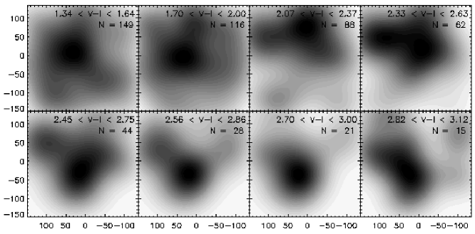
Figure 3: The results of the cluster-finding algorithm in the 3C 254 field. The panels show the smoothed galaxy surface density distribution as a function of predicted colour-magnitude relations at different redshifts. The redshifts are, from top-left to bottom-right, $z=0.2$ to 0.9 in steps of $\Delta z=0.1$. The numbers on each plot show the colour range we assumed that observed $L^{*}$ elliptical galaxies would have at each redshift, as well as the number of galaxies in each colour range (see text for details). Axis units are offset from the quasar in arcsec, and there are 30 greylevels in each panel, defined to span the range from maximum to minimum. North is up and east is to the left.

In order to investigate this in more detail, we derived the surface density distribution of the galaxies as a function of colour. We followed the approach by Gladders & Yee [Gladders & Yee 2000], who have constructed an algorithm to search for clusters in two-filter data (the ‘Red-Sequence Cluster Survey’). Galaxies on a cluster red sequence will be redder than any normal foreground galaxies provided the two filters straddle the 4000 Å break in the rest frame of the cluster. In this manner, $V$- and $I$-filters can be used to search for clusters at $z\approx 0.4$–0.9. We did not implement the whole algorithm since we are not doing a large blank field survey, but merely a simplified version of the first part which assigns probabilities to the galaxies according to whether they are likely to lie in a certain colour interval. If there is a concentration in the surface density of galaxies in a particular colour interval, it classifies as a cluster candidate. The colour interval will then be an indirect indicator of the cluster redshift.

To implement this, we defined colour-magnitude relations between $z=0.20$ and 0.95 for every $\Delta z=0.05$. The zero points of the predicted relations were taken to be equal to the $V-I$ colour of an $L^{*}$ elliptical galaxy at the redshift in question. This was kindly provided by T. Dahlén from his photometric redshift code, which convolves different galaxy templates with the NOT filters [Dahlén, Fransson & Näslund 2002]. The slope of the colour-magnitude relation was taken to vary slightly with redshift, as predicted by Kodama et al. [Kodama et al. 1998] for their elliptical evolution model with a formation redshift of $z_{f}=4.5$. We took the scatter about the colour-magnitude relation to be $\Delta\left(V-I\right)=0.3$ so that it roughly matches the intrinsic scatter and the photometric errors, the latter clearly dominating.

We identified galaxies likely to belong to the defined red sequences by selecting those that had a certain probability of lying in the colour interval, $\left<c_{1},c_{2}\right>$, associated with each sequence. This probability was evaluated as the integral from $c_{1}$ to $c_{2}$ of a normal distribution with mean equal to the measured $V-I$ and dispersion equal to the measurement error in $V-I$ (for details, see Gladders & Yee 2000). Thereafter, we evaluated the surface density distribution of galaxies above a given probability and smoothed it with a Gaussian of width 200 pixels (the same as we use in the mass maps). The result is shown in Fig. 3, where each panel corresponds to a colour-magnitude relation at a given redshift. In order to find a potential cluster in these plots, we looked for well-defined peaks in the surface density within a narrow colour range.

We find two distinct peaks in this figure. In moving from bluer toward redder colours, the first peak turns up at $2.07<V-I<2.37$, 70–80 arcsec N of the quasar. If this is a cluster red sequence, it is predicted to have a redshift of $z\approx 0.4$. The second isolated peak shows up in the two panels spanning the colour range $2.56<V-I<3.00$, and if these galaxies are early-type members of a cluster, the predicted redshift is $z\approx 0.7$–0.8. It is thus possible that the second peak might be a cluster associated with the quasar. Interestingly, the cluster does not seem to be centered on the quasar, but rather 40–50 arcsec to the S. If the quasar is associated with a strong cooling flow (Forbes et al. 1990; Crawford & Vanderriest 1997) in a cluster, we would expect it to lie at the cluster centre where the gravitational well is deep. However, it cannot be ruled out by our data that the cluster might have a slightly higher redshift than 0.734, but it is unlikely that the redshift is higher than 0.85–0.9.

5 Weak lensing analysis

A cluster of galaxies has a high enough mass density to cause deflection of light rays from distant galaxies behind it, thereby distorting their shapes. Depending on the surface mass density of the cluster and the alignment of the background galaxies with the cluster centre of mass and the observer, different levels of distortions are seen – from giant arcs and arclets to only weakly altered galaxy shapes.

Giant arcs are produced in the strong lensing regime when there is good alignment and the surface mass density in the cluster centre is equal to or larger than the critical surface mass density, $\Sigma_{\rm c}$,

$$\Sigma_{\rm c}=\frac{c^{2}}{4\pi G}\frac{D_{\rm s}}{D_{\rm d}D_{\rm ds}}.$$ (1)

Here $D_{\rm s}$ and $D_{\rm d}$ are the angular diameter distances to the source (background galaxy) and the deflector (the cluster), respectively, and the deflector–source angular diameter distance is $D_{\rm ds}$. The weak lensing regime is characterized by the condition $\kappa=\Sigma/\Sigma_{\rm c}\ll 1$, and in this case the background galaxies are only weakly distorted. To detect this effect, we need to measure the ellipticities of a large number of galaxies and look for a systematic shift, in particular for a tangential alignment of the galaxy shapes around the cluster centre.

As opposed to giant arcs, weak lensing occurs in every cluster, but is difficult to quantify because the background galaxies themselves have an intrinsic distribution of ellipticities. This is the main source of noise in weak lensing analysis. In addition to this, the faint galaxies are smeared by the seeing PSF which will circularize the galaxy images and suppress the weak shear signal. There may also be anisotropies in the PSF causing it to change as a function of position in the image. This might be caused by e.g. camera distortions, guiding errors, or strong winds giving rise to vibrations in the mirror or shaking of the telescope. Also, the strain in the instrument caused by its own weight changes direction as the telescope tracks an object across the sky, and this can have an effect on the shapes of the galaxies.

Fortunately, well-developed techniques for measuring galaxy ellipticities and correcting for PSF smearing and anisotropy exist. Here, we use the imcat software by N. Kaiser in which the techniques described by Kaiser et al. [Kaiser et al. 1995] are implemented. imcat detects objects by smoothing the images with a range of Mexican hat filters with different radii. The detection with the highest significance is entered into the catalogue along with parameters such as magnitude, the radius $r_{\rm g}$ of the smoothing filter which maximized the detection significance, and ellipticity. Galaxy ellipticities are evaluated as

$$e_{1}=\frac{Q_{11}-Q_{22}}{Q_{11}+Q_{22}}\hskip 28.45274pte_{2}=\frac{2Q_{12}}{Q_{11}+Q_{22}},$$ (2)

where the elements of the Q matrix are formed from the weighted second moments of the surface brightness.

In each image, we examined the result of the imcat detection process, and made masks when necessary to eliminate spurious objects. In order to include only galaxies likely to have well-determined shapes in the weak lensing analysis, we accepted only galaxies that satisfied the following criteria: 1) $r_{g}$ larger or equal to the stellar radius, but less than six times the stellar radius, 2) significance of detection ($\nu$) greater than six, and 3) corrected ellipticity less than three (see Section 5.1 for a description of the ellipticity corrections). Stars with $I<22$ were separated from galaxies on the basis of a plot of half-light radius versus magnitude, as shown in Fig. 4, and removed from the catalogues. No attempt was made to separate stars from galaxies at $I>22$. At these faint magnitudes, the surface density of galaxies is larger than that of stars by a factor of $>20$ (Reid et al. 1996), so the inclusion of faint stars will not affect our analysis. Bright foreground galaxies and probable cluster members were also taken out of the catalogues by making the cuts in magnitude and colour as described in Section 4. The number of galaxies left for the weak lensing analysis was typically $\sim$1000, see Table 3.

5.1 Shear measurements

In the absence of photon counting noise, the observed ellipticity of a galaxy, $e^{\rm obs}_{\rm i}$, can be expressed as

$$e^{\rm obs}_{\rm i}=e^{\rm s}_{\rm i}+P^{\gamma}_{\rm ij}\gamma_{\rm j}+P^{\rm sm}_{\rm ij}p_{\rm j},$$ (3)

where $e^{\rm s}_{\rm i}$ is the intrinsic ellipticity of the galaxy, the second term is the shift in ellipticity caused by the gravitational shear, $\gamma_{\rm i}$, and the third term describes the smearing of the galaxy image with an anisotropic PSF. The $P^{\gamma}$ and the $P^{\rm sm}$ factors are the shear and the smear polarizabilities, respectively, and are determined by the getshapes routine in imcat, along with the ellipticities $e_{\rm i}^{\rm obs}$ (for details, see e.g. Kaiser et al. 1995; Clowe et al. 2000).

Figure 4: Half light radius versus magnitude of objects in the E1821$+$643 field. Stars are easily identified as the objects on the horizontal branch stretching from $I\approx 15$ to 20–21. At $I\la 15$, the stars saturate and the branch turns upwards.

By applying Eq. 3 to stars which are intrinsically circular ($e^{\rm s}_{\rm i}=0$) and not affected by gravitational shear ($\gamma_{\rm i}=0$), an estimate of ‘stellar shear field’, $p_{\rm i}$, can be made. To do this, we identified unsaturated, bright stars in the images by their half light radii as seen in Fig. 4. The stars were used to investigate the variation of the PSF across the field by fitting a second order polynomial to $p_{\rm i}$ using the imcat task efit. The polynomial was thereafter applied to the galaxies by adjusting their ellipticities with an amount $\delta e_{\rm i}=-P^{\rm sm}_{\rm ij}p_{\rm j}$ using the task ecorrect.

We experimented with higher order polynomials, but found that in most fields there were too few stars to allow this. A second order polynomial was however found to be satisfyingly correcting for any anisotropies. As an example, we show in Fig. 5 the ellipticities of the stars in the E1821$+$643 field before and after the correction. This field has elliptical stars with systematic ellipticities up to $\sim 2$–3 per cent in one direction, but it is seen that the systematics have been successfully corrected for, and that the star ellipticities are reduced to typically $<1.5$ per cent.

In the 3C 295 field, we found systematic ellipticities of $<2$–3 per cent before correction. The stars in the 3C 254 and the 3C 334 fields, which were taken on the same observing run, have systematic ellipticities of up to $\sim 5$ per cent in one direction. We had exceptionally good seeing during this run, down to 0.4 arcsec, and experienced problems with focusing the telescope owing to an almost undersampled PSF. It is possible that the focussing problems might have caused the stars to become slightly elliptical. There was also strong wind part of the time that might have caused vibrations in the mirror and also given rise to the focussing problems. However, in all the fields, we were able to successfully correct for the systematics with residual ellipticities of $<1$–2 per cent uniformly scattered around zero.

Figure 5: Ellipticities of stars before and after correction for PSF anisotropy in the E1821$+$643 field. Perfectly circular stars have $e_{1}=e_{2}=0$.

In the next step, we corrected for the dilution of galaxy ellipticities caused by the smearing by the seeing disk. This step is done in order to convert the observed ellipticities to a gravitational shear. We followed the approach by Luppino & Kaiser [Luppino & Kaiser 1997], which is also described elsewhere (e.g. Clowe et al. 2000). The pre-seeing shear polarizability is defined as

$$P^{\gamma}_{\rm ij}=P^{\rm sh}_{\rm ij}-P^{\rm sm}_{\rm ik}\frac{P^{\rm sh\star}_{\rm kl}}{P^{\rm sm\star}_{\rm lj}},$$ (4)

where the asterisks denote values for stars. Under the assumption that the PSF is close to circular after the correction, the off-diagonal elements of the polarizabilities are small compared to the diagonal elements, so the polarizabilities can be approximated by $P=\frac{1}{2}\left(P_{11}+P_{22}\right)$. We therefore calculated the average $P^{\rm sh\star}/P^{\rm sm\star}$ for stars as

$$\left<\frac{P^{\rm sh}}{P^{\rm sm}}\right>^{\star}=\frac{1}{N_{\rm stars}}\sum_{\rm stars}\frac{P^{\rm sh\star}_{11}+P^{\rm sh\star}_{22}}{P^{\rm sm\star}_{11}+P^{\rm sm\star}_{22}},$$ (5)

and evaluated the pre-seeing shear polarizability as

$$P^{\gamma}=\frac{1}{2}\left(P^{\rm sh}_{11}+P^{\rm sh}_{22}\right)-\frac{1}{2}\left(P^{\rm sm}_{11}+P^{\rm sm}_{22}\right)\left<\frac{P^{\rm sh}}{P^{\rm sm}}\right>^{\star},$$ (6)

where $P^{\rm sh}$ and $P^{\rm sm}$ are provided by imcat.

The gravitational shear was thereafter found by computing

$$\gamma_{\rm i}=\frac{e_{\rm i}}{P^{\gamma}},$$ (7)

so in order to convert the galaxy ellipticities to a shear, a correction factor of $1/P^{\gamma}$ was applied. Each galaxy has a $1/P^{\gamma}$ factor associated with it, and in principle it is possible to correct for PSF dilution on a galaxy-by-galaxy basis. As this tends to be very noisy, we followed the approach by Hoekstra et al. [Hoekstra et al. 1998] by evaluating the correction factors as a function of magnitude and galaxy size instead. We split the galaxies into bins in $r_{g}$ and magnitude such that approximately 20–40 galaxies fell in each bin, and computed the median $1/P^{\gamma}$ for each bin. Typically, the widths of the bins were 0.5–1.0 mag in magnitude and 0.2–0.5 pixels in size.

The bins containing the faintest and smallest galaxies, those that are most affected by the seeing, had the largest correction factors, typically 8–12, whereas a value of unity was reached for larger galaxies which are less affected by seeing. Since the galaxies with the largest correction factors are also the ones with the poorest shape determinations, we assigned weights to the galaxies. For each bin, a normalized weight inversely proportional to the dispersion in $P^{\gamma}$ was calculated, and during the whole analysis, galaxies with poorly determined $1/P^{\gamma}$ were given less weight.

Due to the mass-sheet degeneracy (a uniform sheet of mass can be added without altering the shear), the quantity that we measure from galaxy images is in reality the reduced shear, $g$,

$$g=\frac{\gamma}{1-\kappa},$$ (8)

i.e. a combination of shear, $\gamma$, and convergence, $\kappa$. Since we are working in the weak lensing limit where $\kappa\ll 1$, we use the approximation that $g\approx\gamma$. The shear field can therefore be directly inverted to give the dimensionless projected surface mass density of the cluster.

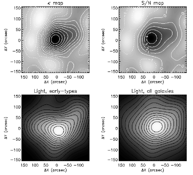
Figure 6: E1821$+$643. The two upper panels show the results of the mass reconstruction. To the left is the map of the projected surface mass density, $\kappa$, and to the right, the signal-to-noise map of the reconstruction. The two lower panels show the distribution of light from the colour-selected early-type galaxies (left) and from all the galaxies in the field (right). In all panels, 60 grey levels were used, spanning from minimum to maximum. The spacing between the $\kappa$ contours is 0.014, and the signal-to-noise contours are labeled with their respective values. Negative contours are drawn with dotted lines. The quasar position is $(\Delta x,\Delta y)=(0,0)$. North is up and east is to the left.

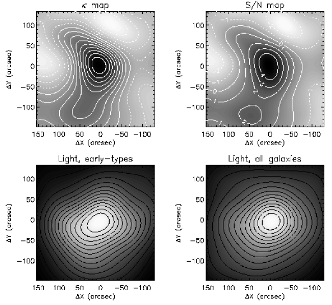
Figure 7: 3C 295. The radio galaxy has coordinates $(\Delta x,\Delta y)=(0,0)$, and the spacing between the $\kappa$ contours is 0.013. For more information about the plots, see text and caption of Fig. 6.

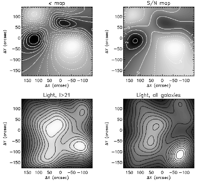
Figure 8: 3C 334. Surface mass density and light distribution, see caption of Fig. 6. The quasar has coordinates $(\Delta x,\Delta y)=(0,0)$, and the spacing between the $\kappa$ contours is 0.014.

5.2 Cluster inversion

We used the original ‘KS93’ inversion technique [Kaiser & Squires 1993] to reconstruct the surface mass density from the shear field. The KS93 algorithm determines the $\kappa$ field to an unknown additive constant and suffers somewhat from biasing at the edges because of the finite field of view. However, it is easy to implement and has well-defined noise properties since the intrinsic ellipticity distribution is translated to white noise across the field. The surface mass density in each cluster was reconstructed on an 82$\times$82 grid with a smoothing length of 200 pixels, corresponding to 38 arcsec. The typical resolution in the mass maps is therefore $\approx 200-300h^{-1}$ kpc at the cluster redshifts.

To quantify the significance of the reconstructions and to test the reliability of the mass maps, we made signal-to-noise maps of the mass reconstructions of each cluster. This was done by generating 100 mass maps by randomly redistributing the measured shear values of the galaxies while keeping their positions. A noise map was made by calculating the rms in each reconstruction point, $\vec{\theta}$, as

$$\kappa_{rms}\left(\vec{\theta}\right)=\sqrt{\frac{\sum_{\rm i=1}^{100}\kappa_{\rm i}\left(\vec{\theta}\right)^{2}}{100}}.$$ (9)

The noise maps show the expected noise level due to the random intrinsic ellipticities of the galaxies. Finally, a signal-to-noise map was made by dividing the original mass map with the noise map.

Table 3: The lens redshift, the weighted average $\left<\beta\right>$ and the corresponding redshift, $z_{\rm sheet}$, for each field. The last column lists the number density of galaxies used in the weak lensing analysis.

Field	$z_{\rm lens}$	$\left<\beta\right>$	$z_{\rm sheet}$	$n$ (arcmin-2)
E1821$+$643	0.297	0.480	0.71	41.40
3C 295	0.460	0.322	0.80	50.65
3C 334	0.555	0.175	0.73	19.86
3C 254	0.734	0.236	1.13	41.57

6 Results

6.1 Mass maps

The mass reconstructions and their signal-to-noise maps are shown in Figs. 6, 7, 8 and 9, in order of increasing quasar redshift. For comparison, we also show the distribution of light in the fields. The early-type light distribution in the E1821$+$643 and the 3C 295 cluster was calculated by selecting galaxies that lie within $1\sigma$ of the derived colour-magnitude relations, whereas for the 3C 254 field, we selected galaxies in the colour range $2.5<V-I<3.5$. Next to the early-type light distributions, we have plotted the light from all galaxies with $I>17$.

6.1.1 E1821$+$643

As seen in Fig. 6, the cluster is comfortably detected, and the mass peak has a signal-to-noise of 4.9. The mass distribution peaks approximately 11 arcsec E of the quasar, but the offset is too small to be significant. Probably, the peak is shifted because of random noise in the reconstruction.

The cluster appears to have a relatively smooth mass distribution. The mass contours show an extension to the NW which is present at a signal-to-noise level of 2–3 (the resolution is $\approx 200h^{-1}$ kpc). It is likely that this is a feature of the cluster, since the same asymmetry is present in the early-type light distribution. And, as expected, it is seen to be more or less washed out when we plot the light distribution of all the galaxies (the quasar host galaxy is not included in the light distribution since it is saturated). The ROSAT PSPC X-ray image published by Saxton et al. [Saxton et al. 1997] appears to be slightly extended in the same direction as the mass map. An apparent ellipticity of the cluster was also noticed in X-rays by Hall et al. [Hall et al. 1997], but it is not clear whether this ellipticity corresponds to the feature seen in the mass map. A recent Chandra image published by Fang et al. [Fang et al. 2001] also shows ellipticity to some degree.

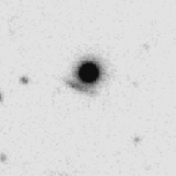
Figure 10: A probable $z\sim 1$ galaxy being lensed by a combination of the E1821$+$643 cluster potential and the gravitational potential from an elliptical cluster member. To the left is shown the elliptical galaxy with the candidate lensed galaxy $\approx$3 arcsec to the SE (the J2000 coordinates of the ‘lensed’ galaxy are 18:21:59.6 and $+$64:19:47.6), and in the image to the right the elliptical has been subtracted. North is up, and east is to the left.

We find a strong lensing candidate in this cluster. An elliptical galaxy which belongs to the cluster (spectroscopically confirmed by Schneider et al. (1992), galaxy ‘H’ in their paper) has a close, very elongated neighbour 3 arcsec to the SE, see Fig.10. The neighbour is slightly curved around the elliptical galaxy and could thus be lensed by a combination of the cluster potential and the potential from the cluster member. By masking out the ‘lensed’ galaxy and making a model of the elliptical cluster member using the stsdas tasks ellipse and bmodel, we subtracted the elliptical from the image and performed photometry on the ‘lensed’ galaxy. We found an $I$-magnitude of 21.09 and colours $V-I=3.15$ and $B-V=0.55$. Judging from the red $V-I$ colour, the 4000 Å break probably lies at a redshifted wavelength of $\sim$8000 Å, thus placing the galaxy at $z\sim 1$. When properly modeled, cases like this can be used to put constraints on the mass distribution and dark matter content in galaxies (e.g. Lubin et al. 2000).

6.1.2 3C 295

The distribution of the surface mass density and the galaxy light in the 3C 295 cluster is shown in Fig. 7. Also this cluster appears smooth in the mass map. Again, the mass peak is slightly offset ($\approx$7 arcsec to the E) from the position of the central radio galaxy, but we attribute this to random noise in the reconstruction. The peak is detected at a signal-to-noise level of 5.0, and the cluster appears somewhat elongated in the NS direction. Neumann [Neumann 1999], who observed the cluster in X-rays with the ROSAT HRI also note the elongation, but in the Chandra X-ray image taken by Allen et al. [Allen et al. 2001] this is not seen.

There is evidence for strong lensing also in this cluster. We find a candidate gravitational arc 25 arcsec W and 10 arcsec N of the radio galaxy, the J2000 coordinates are 14:11:17.9 and $+$52:12:21.8. It is detected in $I$, but not in the $V$ image. Smail et al. [Smail et al. 1997a] make a note in their paper that the cluster displays signs of strong lensing, but do not give the position of the arc. However, an arc is clearly visible in the WFPC2 image at this position, so this must be the arc found by Smail et al. Gravitational arcs are usually found close to cluster centres at approximately the Einstein radius. If we take the Einstein radius to be at the position of the arc, the Einstein radius is $\approx 22$ arcsec, corresponding to 75$h^{-1}$ kpc. Assuming that the cluster core is a singular isothermal sphere and that the arc lies at a redshift of $z_{\rm source}=1.0$, the mass enclosed within the Einstein radius is $1.02\times 10^{14}h^{-1}$ M_⊙. For an arc redshift of $z_{\rm source}=2$, the enclosed mass is $7.1\times 10^{13}h^{-1}$ M_⊙. Upon identification of any counter images and further modeling, tighter constraints can be made on the mass and the mass distribution in the cluster core.

6.1.3 3C 334

The result of the cluster reconstruction in the 3C 334 field is shown in Fig. 8 along with the light distribution of $I>21$ and $I>17$ galaxies. As noted before, this field is not deep enough to obtain a reliable weak lensing result. We applied the same selection criteria in this field as for the other fields, except that we allowed a slightly brighter magnitude cut at $I=20$ (we also tried with $I=21$), but as seen in Table 3 there are very few galaxies in this field compared to the other three fields. The completeness limit is $I\approx 23.5$, whereas a limit of $I\approx 25$ is preferred since most of the galaxies contributing to the weak lensing signal have $I\approx 23$–26. Our current data can therefore neither confirm nor exclude the presence of a cluster in this field.

The cloverleaf-like pattern in the mass map may originate in the complex kernel in the reconstruction algorithm, and trying to reconstruct a mass map based on just one galaxy would produce a similar pattern. However, the eastern peak in the mass map looks significant, so it could be caused by a foreground mass concentration, but it is not supported by the galaxy light distribution. It is possible that there is some systematic error in these data that we do not yet understand.

6.1.4 3C 254

This is the most interesting field, both because of the relatively high redshift of the quasar, and because there is a concentration of red galaxies in the image that may correspond to a cluster at the quasar redshift (see Section 4.1). As seen in Fig. 9, we have made a significant detection of mass in this field. The mass peak in the $V$-band image has a signal-to-noise of 2.8. Even though the $I$-band image is somewhat shallow with a completeness limit of $\approx 24$, there is also a detection of mass in this image, although it is marginally significant with a signal-to-noise of $\approx 2$.

The $V$- and the $I$-band mass maps are seen to peak at different places, approximately 47 arcsec apart, but we consider it unlikely that they originate in different mass concentrations. Taking into account the level of noise in the reconstructions, they both probably correspond to the same cluster. The $V$-band mass map, which is the most reliable reconstruction, peaks 21 arcsec E and 34 arcsec S of the quasar. If the positional accuracy of the peak is related to signal-to-noise as $\sim$smoothing length/signal-to-noise, the 1-$\sigma$ error in the peak position is $\sim 15$ arcsec. The position of the mass peak might therefore be consistent with the position of the quasar.

We note that the mass peak lies closer to the peak in the early-type galaxy light; the separation between the two is $\approx 10$ arcsec. The early-type galaxy light corresponds to the concentration of red galaxies that was discussed in Section 4.1 as a possible cluster at the quasar redshift. In this relatively noisy reconstruction it is unfortunately not possible to tell whether the cluster is centered on the quasar, or on the peak in the early-type light.

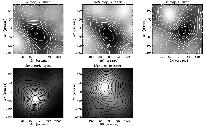
Figure 9: 3C 254. The upper row of panels shows, from left to right, the $V$-band mass map, its signal-to-noise map, and the $I$-band mass map. The mass peak in $V$ has a signal-to-noise of 2.8, whereas the mass peak in $I$ has a signal-to-noise of 1.9 (the $I$-band signal-to-noise map is not shown here). The spacing between the $\kappa$ contours is 0.018 and 0.007 in the $V$- and the $I$-band mass map, respectively. In the two lower panels are shown the light distribution of colour-selected ($2.5<V-I<3.5$) galaxies and of all $I<21$ galaxies. The quasar has coordinates $(\Delta x,\Delta y)=(0,0)$. See Fig. 6 for more details about the plots.

6.2 Tangential shear and mass profiles

We now derive the surface mass density and mass profiles of the clusters using the aperture mass densitometry method (Fahlman et al. 1994; Kaiser et al. 1994). This method converts the tangential component of the shear to a surface mass density profile, which is thereafter used to obtain a lower limit on the mass as a function of radius.

Figure 11: E1821$+$643. The two upper plots show the tangential, $\left<g_{\rm T}\right>$, and the orthogonal shear, $\left<g_{\rm X}\right>$, as a function of radius. Below is shown their respective $\zeta$-estimators, denoted $\zeta_{\rm T}$ and $\zeta_{\rm X}$, and the corresponding mass profiles. The inner radius was taken to be 35 arcsec and the outer radius of the control annulus was 164 arcsec. The best-fit SIS model with velocity dispersion 964${}^{+149}_{-176}$ km s^-1 is plotted as the solid and the two dashed lines in the upper left-hand plot.

First, we evaluated the azimuthally averaged tangential shear, $\left<g_{\rm T}\right>$, in annuli centered on the peak in the mass maps. The tangential component of the shear is $g_{\rm T}=-g_{1}\cos(2\phi)-g_{2}\sin(2\phi)$, where $\phi$ is the azimuthal angle of the galaxy with respect to the chosen centre. Thereafter, we calculated the $\zeta$-estimator which gives the mean dimensionless surface mass density within a radius $r_{\rm j}$ relative to that in an outer control annulus at $r_{\rm j}<r<r_{\rm max}$:

$$\zeta(r_{\rm j},r_{\rm max}) = \bar{\kappa}(<r_{\rm j})-\bar{\kappa}(r_{\rm j}<r<r_{\rm max})$$ (10)

$$= \frac{2}{(1-r_{\rm j}^{2}/r_{\rm max}^{2})}\int_{r_{\rm j}}^{r_{\rm max}}{\rm d}\ln r\left<g_{\rm T}\right>.$$

The $\zeta$-statistic gives a lower limit to the mass within some radius since the mass in the control annulus always will be different from zero. In order to get a good measurement of the mass it is therefore desirable to have a wide field so that $r_{\rm j}/r_{\rm max}\ll 1$.

We used the peak in the mass maps as centre for the annuli, and took the outer radius, $r_{\rm max}$, to be as large as possible without loosing too much of the area of the outer control annulus. The inner radius was typically 35 arcsec, sufficiently outside the Einstein ring for each cluster to assure that the weak lensing approximation was valid. The $\zeta$-statistic is less well applicable to fields with two or more peaks in the mass distribution since the mass for one peak will be biased downwards when the other peak lies in the control annulus. The mass measured with this technique therefore depends both on the strength of the shear signal and on the mass profile of the cluster.

In Figs. 11 through 13, we show the results of the aperture mass densitometry and the mass profiles for each cluster (from now on, we do not discuss the 3C 334 field). The left-hand panels show, from top to bottom, the average tangential shear profile, $\left<g_{\rm T}\right>$, its $\zeta$-estimator, $\zeta_{\rm T}$, and its mass profile. The right-hand panels show the corresponding quantities, but for the orthogonal shear component, $\left<g_{\rm X}\right>$. The orthogonal shear was found by rotating the galaxies 45 degrees, or equivalently, increasing the phase of the shear by $\pi$ radians. It gives a measure of the random shear component caused by the intrinsic ellipticities of the galaxies, and the variance in $g_{\rm X}$ was therefore used as a measure of the error in $g_{\rm T}$ [Luppino & Kaiser 1997]. To ensure that the weak tangential shear originates in gravitational lensing and not some other systematic effect, a good check is that the orthogonal shear component be zero within the statistical uncertainty. Note that the points and the error bars for the $\zeta$-statistic (hence also the mass) are correlated since $\zeta(r_{\rm j},r_{\rm max})$ gives the mean surface density interior to $r_{\rm j}$ relative to the mean in the outer control annulus. As seen in Figs. 11 through 13, there is a positive tangential shear detected in the three clusters, and the orthogonal shear component is scattered around zero, as expected if the weak shear is caused by gravitational lensing.

The mass profiles were calculated from the $\zeta$-statistic by evaluating $M(<r_{\rm j})=\pi r_{\rm j}^{2}\zeta(r_{\rm j},r_{\rm max})\Sigma_{\rm c}$. It is thus seen that the critical surface mass density, $\Sigma_{c}$, has to be known in order to convert to an absolute measure of mass. From Eq. 1, $\Sigma_{\rm c}$ can be seen to depend on the redshift distribution of the weakly lensed galaxies through the ratio $\beta\equiv D_{\rm ds}/D_{\rm s}$. This ratio is in principle unknown, at least at magnitudes fainter than $I\approx 23$. We can however make a reasonable estimate of the redshift distribution of faint galaxies by using the photometric redshifts that are available in the Hubble Deep Field (HDF).

For this, we used the HDF photometric redshift catalogue by Fernández-Soto, Lanzetta & Yahil (1999) which contains $\approx 1000$ galaxies, and followed the approach of Dahle et al. [Dahle et al. 2002] by comparing the number counts of galaxies in the cluster images with the number counts in the HDF.

The $F814W_{AB}$ magnitudes were first converted onto the STMAG system using the tabulated values in the HDF web pages, and thereafter to Cousins $I$ using the prescription in the WFPC2 Instrument Handbook [Biretta et al. 2000]. Since we used the $V$-magnitudes in the 3C 254 field, we also transformed from $F606W_{AB}$ to Johnson $V$ with the conversion $V-F606W_{AB}=-0.09$ (found by using the stsdas.synphot task to transform a galaxy with spectrum $F_{\nu}\propto\nu^{-1}$).

We grouped the galaxies in the cluster images and in the HDF into magnitude bins of width 0.5 between the magnitude limit used in the weak lensing analysis and a faint limit of $I=26$ or $V=27$. Galaxies fainter than this were counted in one bin. For each HDF magnitude bin, a mean $\beta$ was calculated using the photometric redshifts. Thereafter, we weighted $\beta$ in each bin with the normalized weights associated with the galaxies in the cluster images within the same bin. The weighted $\beta$ values were finally added and a single weighted average $\left<\beta\right>$ was calculated for each cluster. This is equivalent to putting the source population at a sheet behind the cluster. In Table 3, we list the values of $\left<\beta\right>$ that we used, and the corresponding sheet-redshifts.

Figure 12: 3C 295. Tangential and orthogonal shear and their respective $\zeta$-estimators and mass profiles. Inner and outer radii were 35 and 151 arcsec, respectively. The two asterisks at a radius of 22 arcsec in the lower left-hand plot correspond to the mass estimated by strong lensing. The upper and lower asterisk symbols correspond to an assumed arc redshift of $z=1$ and $z=2$, respectively. Overplotted on the shear profile, $\left<g_{\rm T}\right>$, is the best-fit SIS model with $\sigma_{v}=1205^{+161}_{-187}$ km s^-1 (solid and dashed lines).

Figure 13: 3C 254. Tangential and orthogonal shear and their respective $\zeta$-estimators and mass profiles. The inner radius was 35 arcsec, and the outer radius 142 arcsec. The solid and the dashed lines in the upper left-hand plot shows the best-fit SIS model with a velocity dispersion of $\sigma_{v}=1244^{+243}_{-302}$ km s^-1.

For the 3C 295 cluster, we find a mass of $(2.86\pm 1.74)\times 10^{14}h^{-1}$ M_⊙ within a radius of 407$h^{-1}$ kpc. This agrees well with the mass estimate by Smail et al. [Smail et al. 1997a] of $(2.35\pm 0.38)\times 10^{14}$ $h^{-1}$ M_⊙ within 400$h^{-1}$ kpc. Using Chandra X-ray data, Allen et al. [Allen et al. 2001] derive a mass of $1.05^{+0.40}_{-0.25}\times 10^{14}h^{-1}$ M_⊙ within the same radius. Our estimate is thus in better agreement with Smail et al., but since our error bars are large, it is also consistent with the mass found by Allen et al. Allen et al. discuss the discrepancy between the X-ray and lensing mass as possibly originating in mass along the line of sight which is detected via weak lensing, but not in X-ray images. There is however a possibility the outermost point in our mass profile of 3C 295 might be overestimated because of the inclusion of the secondary peak to the south in the mass map. The mass within 300$h^{-1}$ kpc is $(1.38\pm 1.09)\times 10^{14}h^{-1}$ M_⊙, more in agreement with Allen et al.’s X-ray mass estimate.

The E1821$+$643 cluster is massive too, with a mass of $(1.51\pm 1.24)\times 10^{14}h^{-1}$ M_⊙ within a radius of $\approx 400h^{-1}$ kpc, but the most massive cluster appears to be that in the 3C 254 field, with a mass of $(4.28\pm 2.86)\times 10^{14}h^{-1}$ M_⊙ within $\approx 400h^{-1}$ kpc. The masses within radii of 200$h^{-1}$ and 400$h^{-1}$ kpc in the three clusters are listed in Table 4.

There are several factors which may give rise to systematic errors in the mass. The value of $\left<\beta\right>$ affects the mass, both through the redshift distribution of the faint background galaxies and through the assumed cosmology. If the weakly lensed galaxies lie at systematically higher redshifts than assumed here, $\left<\beta\right>$ will be larger, so the clusters should be less massive. For instance, if the source population for the 3C 295 cluster is redshifted out to $z_{\rm sheet}=1$ instead of $z_{\rm sheet}=0.8$ as assumed, the mass within 400$h^{-1}$ kpc will be $(2.25\pm 1.36)\times 10^{14}h^{-1}$ M_⊙. We have assumed an Einstein-deSitter Universe with $q_{0}=0.5$ and $\Omega_{0}=1$, but in a flat Universe with $\Omega_{\Lambda}=0.8$ and $\Omega_{\rm m}=0.2$, both $\left<\beta\right>$ and $D_{\rm d}$ will be larger by a factor of $\approx 1.2$–1.3, thus giving masses smaller by a factor of $\approx 1.2^{2}$–$1.3^{2}$.

The tangential shear is given by $\left<g_{\rm T}\right>=-{\rm d}\kappa/{\rm d}\ln\theta$, and for a singular isothermal sphere (SIS), the surface mass density, $\kappa$, is proportional to the velocity dispersion, $\sigma_{v}^{2}$. The shear profiles were therefore used to estimate the velocity dispersions of the clusters by minimizing $\chi^{2}$. SIS models with the best-fit velocity dispersions and their 68 per cent confidence intervals are overplotted on the tangential shear profiles in Figs. 11 to 13, and we also list the results of the fitting in Table 4.

The velocity dispersions we find are generally lower than those measured spectroscopically. Dressler et al. [Dressler et al. 1999] measure $\sim 1630$ km s^-1 for the 3C 295 cluster, whereas we derive a best-fit SIS model with $\sigma_{v}=1205^{+161}_{-187}$ km s^-1. Likewise, for the E1821$+$643 cluster, we find $\sigma_{v}=964^{+149}_{-176}$ km s^-1 from the SIS fit, but 1180 km s^-1 from spectroscopy of galaxies in the field (Schneider et al. 1992; Le Brun et al. 1996; Tripp et al. 1998). The discrepancy between the two methods of measuring velocity dispersions was noted by Smail et al. [Smail et al. 1997a], who suggested it could be caused by different velocity dispersions for different galaxy populations. The early-type population has a lower velocity dispersion and is more centrally concentrated than the late-type population. Spectroscopically measured velocity dispersions thus become overestimated since they are often based on galaxies of different types lying at larger distances from the cluster core than that probed by weak lensing. On the other hand, Irgens et al. (2002) found for a sample of 12 clusters with redshifts between 0.15 and 0.33 that estimates of velocity dispersions made from weak gravitational lensing and from direct spectroscopic measurements are in good agreement, with only insignificant systematic bias. Using either technique, however, it is clear that the clusters studied here have very deep potential wells, and are at the upper end of the distribution of Abell cluster velocity dispersions (e.g. Girardi et al. 1998).

Table 4: Physical parameters derived for the AGN host clusters. In the second and third columns are listed the mass within 200$h^{-1}$ and 400$h^{-1}$ kpc, and in column four and five, the result of the SIS fits to the shear profiles.

Cluster	Mass (1014 M⊙)		$\sigma_{v}$ (68 % C.I.)	$\chi^{2}$/dof (dof)
	$<200h^{-1}$ kpc	$<400h^{-1}$ kpc	km s-1
E1821$+$643	1.01$\pm$0.41	1.51$\pm$1.24	964 (788,1113)	0.41 (6)
3C 295	1.44$\pm$0.53	2.86$\pm$1.73	1205 (1018,1366)	0.50 (5)
3C 254	1.63$\pm$0.97	4.28$\pm$2.86	1244 (942,1487)	1.02 (5)

6.3 Mass-to-light ratios

The M/L ratio parameterizes the amount of dark matter in clusters. We have already measured the amount of total mass in the clusters, and by estimating the optical luminosity of the clusters, we may find their M/L ratios. We processed the images in SExtractor with a tophat convolution filter matched to the seeing, and for each extracted object, aperture magnitudes within 2.6 arcsec and ‘best’ magnitudes were evaluated. Stars were identified on the basis of a plot of FWHM versus the SExtractor star-galaxy classifier, and removed from the catalogues by rejecting objects that had a star-galaxy class greater than $\approx 0.8$ and a FWHM corresponding to the seeing. The best seeing catalogue was thereafter matched to the catalogue in the other filter on the basis of object positions, with a tolerance of 3 pixels. A final catalogue was then made containing galaxies detected in both $V$ and $I$ (or $B$, $V$ and $I$ for E1821$+$643).

The galaxy colours were calculated using the aperture magnitudes, and the cluster early-type galaxies were again selected by their location on the colour-magnitude relation. For consistency, we used the same sigma clipping algorithm as described in Section 4 to define the colour-magnitude relations from the SExtractor detections, but obtained very similar results to those listed in Table 2.

The $B$-band luminosity in solar units of each galaxy on the colour-magnitude sequence was evaluated using the ‘best’ $I$ magnitudes converted to absolute $B$ magnitudes by first applying an $I$-band $K$-correction for E/S0 galaxies from Rocca-Volmerange & Guiderdoni [Rocca-Volmerange & Guiderdoni 1988], and thereafter adding the rest-frame $B-I=2.27$ of elliptical galaxies (Fukugita, Shimasaku & Ichikawa 1995). The $K$-corrections applied for the three clusters in order of increasing redshift were 0.18, 0.39 and 0.635. We converted to solar $B$ luminosity by adopting $M_{B\odot}=5.48$.

The procedure to compute M/L ratios as a function of radius is similar to that described for the $\zeta$-statistic; the luminosity density within a given aperture is compared to the luminosity density within a control annulus.

The argument for using the early-type galaxy light to calculate the M/L ratio is that most of the light, and also most of the mass, is associated with the early-type cluster galaxies. Kaiser et al. [Kaiser et al. 1998] find that 70 per cent of the total excess light within their cluster apertures comes from early-type galaxies. They also argue that fairly accurate estimates of cluster luminosities can be obtained from the early-type cluster population since the noise due to foreground and background contamination will be greatly reduced. Smail et al. [Smail et al. 1997a] also point out that using the early-type galaxy light for the M/L ratio makes it easier to compare with other clusters since the blue galaxy fraction is known to vary from cluster to cluster.

Nevertheless, we also calculated the M/L ratio obtained by selecting all galaxies at $I<17$. By subtracting off the luminosity density in the control annulus, any uniform component will be removed, thereby limiting the contamination by field galaxies. In doing this, the galaxies on the colour-magnitude relation were converted to absolute $B$ luminosities as described above, whereas the rest of the galaxies were $K$-corrected assuming an Sa-type galaxy at the cluster redshift and a rest frame colour of $B-I=1.99$ [Fukugita et al. 1995]. The Sa-type $K$-corrections we used were, in order of increasing cluster redshift, 0.09, 0.22 and 0.38 [Rocca-Volmerange & Guiderdoni 1988].

The results for the 3C 295 and the E1821$+$643 clusters are shown graphically in Fig. 14. The errors in the M/L ratio were calculated assuming photometric errors of 0.1 mag in addition to the previously given errors in the mass. The early-type M/L ratios we find for the two clusters 3C 295 and E1821$+$643 lie typically between $\approx$500$h$ and 1000$h$ (M/L)_⊙ at the different radii, and the M/L ratios which include all galaxies are typically 300-500$h$ (M/L)_⊙, depending on the radius. Smail et al. [Smail et al. 1997a] get an early-type M/L ratio in $V$-band of 900$h$ (M/L)_⊙ within 400$h^{-1}$ kpc for the 3C 295 cluster. Assuming an average colour of $B-V=0.78$ for the galaxies, corresponding to that of an Sab-type galaxy (Fukugita et al. 1995), and adopting $(B-V)_{\odot}=0.68$, we get that Smail et al.’s M/L ratio converts to $\approx 987h$ (M/L)_⊙ in $B$-band. This agrees with our estimate of 2050$\pm$1420 (M/L)_⊙ within the same radius.

In the 3C 254 field, we find 39 galaxies with $2.5<V-I<3.5$ within the radius of the outer control annulus. This is clearly too few galaxies to obtain a reliable result with the method described above. The M/L ratio for the 3C 254 cluster is therefore highly uncertain at this point.

We note that the M/L ratios we find are moderately high. The mean early-type M/L ratio obtained by Smail et al. [Smail et al. 1997a] for their ten clusters at $z\approx 0.2$–0.5 is (M/L_V)${}^{\rm early}=483\pm 103h$, and the median is 410$h$ (M/L)_⊙. This corresponds to $\approx 530h$ and $\approx 450h$ in the $B$-band, so the values of $\approx 700h$ we get are moderately high in comparison. When the whole galaxy population is included, it is found that rich clusters where the early-type fraction is high have M/L ratios of typically $\sim 300$–400$h$ (M/L_B)_⊙ (Bahcall, Lubin & Dorman 1995; Carlberg et al. 1997; Dahle et al. 2002, in prep.). Our corresponding number for the E1821$+$643 and the 3C 295 cluster is (M/L${}_{B}^{\rm all}$) $\sim 500h$ (M/L)_⊙.

Figure 14: M/L ratio as a function of radius. Filled symbols correspond to early-type galaxy light and the open symbols correspond to light from all galaxies having $I>17$. The points are shifted slightly in the x-direction for clarity.

7 Discussion

Our results for the 3C 295 cluster are in agreement with what has been found for this cluster previously, i.e. the cluster is massive and has a high velocity dispersion, and the M/L ratio is moderately high. It also shows signs of strong lensing at a radius close to the Einstein radius we would predict from our weak lensing measurements, suggesting that there is a large concentration of mass in the core ($\sim 10^{14}h^{-1}$ M_⊙) and that the cluster potential is deep.

The mass distribution in the E1821$+$643 cluster is relatively smooth, apart from some asymmetry to the NW. The same asymmetry is present in the early-type cluster light, indicating that the feature in the mass map is real. The asymmetry could be caused by a group or a sub-cluster that has fallen in and merged with the main cluster. If this is the case, the merger is probably in a fairly advanced stage since the mass distribution is elongated rather than double-peaked. One of the cluster members in the direction of the asymmetry (41 arcsec N and 15 arcsec W of the quasar) is an FRI radio galaxy. Since FRI galaxies are known be central cluster galaxies (Longair & Seldner 1979; Prestage & Peacock 1988, 1989; Hill & Lilly 1991), we speculate that a sub-cluster or a galaxy group associated with the FRI source has merged with the main cluster. Dynamical activity in clusters is relatively common, more than 30 per cent of clusters show evidence in X-rays of merging [Jones & Forman 1992]. The same fraction of activity is also found in weak lensing studies [Dahle et al. 2002], suggesting that many clusters are still forming by merging of sub-clusters and galaxy groups.

The morphology of the mass distribution in the 3C 254 field is highly uncertain because the reconstruction is relatively noisy, but it appears to be a very massive cluster with a high velocity dispersion, $\sigma_{v}\approx 1200$ km s^-1. Because of random noise, the position of the mass peak is also uncertain, but the position of the peak in the galaxy light distribution is easier to constrain. Galaxies with the expected colours of ellipticals at the quasar redshift are concentrated in a region 40 arcsec S of the quasar. The $I$-band image reaches a completeness limit of $I\approx 23.5$, corresponding to $\approx 2$ magnitudes fainter than $M^{*}$ at the quasar redshift, so the image should be deep enough to trace the most massive galaxies of the early-type population in a $z=0.734$ cluster.

The 40 arcsec offset between the quasar and the peak in the early-type galaxy light (assuming the colour-selected galaxies lie at the quasar redshift) is not what we expect if the quasar sits in a massive cooling flow as suggested by Crawford & Vanderriest (1997). A cooling flow cluster is expected to be evolved and have a deep potential well, and the early-type cluster galaxies should be centrally concentrated. It would therefore be interesting to know where the mass map peaks in relation to the quasar and the early-type galaxy light, but in our reconstruction, the positional errors are too large to address this.

Is it possible that foreground or background structure may contaminate the morphology and the mass estimate of the cluster in the 3C 254 field? We found in Section 4.1 what appears to be a foreground group or cluster, possibly at $z\sim 0.4$, but it lies at a large angular distance from the quasar and is unlikely to have altered the morphology of the mass distribution around the quasar. Also, any background structure at a significantly larger redshift than the quasar would need to have an unrealistically high mass to alter the reconstruction.

The evidence for an association of the detected mass with the 3C 254 quasar is the following: 1) The mass distribution has a peak which is, within the uncertainties, centered on the quasar, 2) there is significant, extended X-ray emission around the quasar (Crawford et al. 1999; Hardcastle & Worrall 1999), 3) the quasar is surrounded by an extended emission-line region which signifies gas under high pressure (Forbes et al. 1990; Crawford & Vanderriest 1997), and 4) there is an apparent excess of galaxies around the quasar [Bremer 1997]. In the rest of the discussion we therefore assume that the cluster is associated with the quasar, but not necessarily centered on it.

How do the clusters we have studied here fit into the interaction/merger scenario and the cooling flow model for fuelling AGN in clusters? Both the distribution of mass and galaxies in the clusters detected at high signal-to-noise, E1821$+$643 and 3C 295, are fairly smooth, and their velocity dispersions are high. Unless there is sub-cluster merging along the line of sight, this indicates that the clusters are evolved and dynamically relaxed. They therefore do not fit well into the scenario where galaxy-galaxy interactions in dynamically young clusters fuel the AGN. Also, the moderately high M/L ratios we find seem to argue against this picture. One might expect that in a young non-virialized cluster, the cluster core would contain a smaller fraction of the total mass since the mass would still not have accumulated there, thus giving a lower M/L ratio than a virialized cluster.

Whereas the 3C 295 cluster is known to contain a cooling flow (Henry & Henriksen 1986; Neumann 1999; Allen et al. 2001), it is less certain that the other two clusters have cooling flows. So, although we cannot rule out the cooling flow model for the clusters, it seems possible that powerful AGN can exist in massive clusters with deep potential wells without being powered by cooling flows. E.g. Hall et al. [Hall et al. 1997] suggested that strong interactions between the AGN host and a gas-rich galaxy is the only necessary mechanism for triggering and fuelling AGN in clusters. However, as pointed out by Hall et al., this predicts that the AGN hosts have disturbed morphology and that the clusters are dynamically young.

If instead interactions between galaxies can occur in dynamically relaxed clusters which have undergone mergers, this could explain our findings. If a merger between two galaxies can push gas into the centre of a galaxy, perhaps a merger between two clusters could result in a whole galaxy being pushed towards the cluster centre. A cluster merger event could thus disrupt the orbits of some galaxies and send them down into the centre of the potential well where the AGN host galaxy sits. If the infalling galaxy is rich in gas, it could end up as a source of fuel for the AGN. Even if the dynamical friction is too low and the infalling galaxy never interacts strongly with the AGN host, it could end up losing gas to the host, or at least disturb the gas in the host galaxy itself. This scenario predicts that systems containing powerful AGN show a high incident of cluster mergers.

The M/L ratios of the clusters studied here seem to be moderately high compared to clusters in general. This could mean that they are indeed very massive and have high X-ray temperatures, typical for old clusters where the mass is more concentrated than the light [Bahcall & Comerford 2002]. Another interesting possibility is that AGN-selected clusters have systematically higher M/L ratios than purely X-ray or optically selected clusters. This might indicate that X-ray and optical surveys are biased toward clusters with high baryon-to-dark matter ratios, and could be important to cosmology as it may affect estimates of $\Omega$ in matter derived from analysis of known clusters [White et al. 1993].

8 Conclusions

Although our sample is too small to draw conclusions about the properties of AGN host clusters in general, we can at least point to some interesting facts about clusters hosting powerful AGN:

1. They can be very massive systems with masses of a few times 10${}^{14}h^{-1}$ M_⊙ within the central $\approx 500h^{-1}$ kpc.

2. They can have very high velocity dispersions of 1000–1600 km s^-1

3. One shows evidence of a cluster merger event (E1821$+$643)

4. Even though the few clusters studied here are consistent with being drawn from the general cluster population, there is some tentative evidence that they tend to have higher M/L ratios than clusters in general

The data presented here do not point unambiguously to either the cooling flow model or the young cluster model for fuelling powerful AGN in clusters. Points i) and ii) above support the cooling flow model since cooling flows are expected to occur in dynamically relaxed clusters with deep potential wells. On the other hand, point iii) argues against the cooling flow model, and more in favour of the young cluster model, although the E1821$+$643 cluster is clearly relaxed.

Our study has demonstrated that it is possible to find and study massive clusters associated with AGN using weak lensing techniques. There seems to be good reasons for expecting moderately rich clusters around the most luminous $z\la 1$ radio sources (e.g. Best 2000), and weak lensing observations in these fields might reveal whether they are indeed surrounded by clusters.

References

- [Allen et al. 2001] Allen S.W., et al., 2001, MNRAS, 324, 842
- [Bahcall & Comerford 2002] Bahcall J.N., Comerford J.M., 2002, ApJ, 565, L5
- [Bahcall et al. 1997] Bahcall J.N., Kirhakos S., Saxe D.H., Schneider D.P., 1997, ApJ, 479, 642
- [Bahcall, Lubin & Dorman 1995] Bahcall N.A., Lubin L.M., Dorman V., 1995, ApJ, 447, L81
- [Beers, Flynn & Gebhardt 1990] Beers T.C., Flynn K., Gebhardt K., 1990, AJ, 100, 32
- [Bertin & Arnouts 1996] Bertin E., Arnouts S., 1996, A&AS 117, 393
- [Best 2000] Best P., 2000, MNRAS, 317, 720
- [Biretta et al. 2000] Biretta J.A., et al., 2000, WFPC2 Instrument Handbook, Version 5.0 (Baltimore: STScI)
- [Blundell et al. 1996] Blundell K.M., Beasley A.J., Lacy M., Garrington S.T., 1996, ApJ, 468, L91
- [Bremer, Fabian & Crawford 1997] Bremer M.N., Fabian A.C., Crawford C.S., 1997, MNRAS, 284, 213
- [Bremer et al. 1992] Bremer M.N., Crawford C.S., Fabian A.C., Johnstone R.M., 1992, MNRAS, 254, 614
- [Bremer 1997] Bremer M.N., 1997, MNRAS, 284, 126
- [Briel & Henry 1993] Briel U.G., Henry J.P., 1993, A&A, 278, 379
- [Canalizo & Stockton 2001] Canalizo G., Stockton A., 2001, ApJ, 555, 719
- [Carlberg et al. 1997] Carlberg, 1997, ApJ, 478, 462
- [Clowe et al. 2000] Clowe D., Luppino G.A., Kaiser N., Gioia I.M., 2000, ApJ, 539, 540
- [Crawford & Vanderriest 1997] Crawford C.S., Vanderriest C., 1997, MNRAS, 285, 580
- [Crawford et al. 1999] Crawford C.S., Lehmann I., Fabian A.C., Bremer M.N., Hasinger G., 1999, MNRAS, 308, 1159
- [Crawford & Fabian 1989] Crawford C.S., Fabian A.C., 1989, MNRAS, 239, 219
- [Dahle et al. 2002] Dahle H., Kaiser N., Irgens R.J., Lilje P.B., Maddox S.J., 2002, ApJS, 139, 313
- [Dahlén, Fransson & Näslund 2002] Dahlén T., Fransson C., Näslund M., 2002, MNRAS, 330, 167
- [Dressler et al. 1997] Dressler A., et al., 1997, ApJ, 490, 577
- [Dressler et al. 1999] Dressler A., Smail I., Poggianti B.M., Butcher H., Couch W.J., Ellis R.S., Oemler Jr. A., 1999, ApJS, 122, 51
- [Dunlop & Peacock 1990] Dunlop J.S., Peacock J.A., 1990, MNRAS, 247, 19
- [Edge et al. 1992] Edge A.C., Stewart G.C., Fabian A.C., 1992, MNRAS, 258, 177
- [Ellingson et al. 1991b] Ellingson E., Yee H.K.C., Green R.F., 1991a, ApJ, 371, 36
- [Ellingson et al. 1991a] Ellingson E., Green R.F., Yee H.K.C., 1991b, ApJ, 378, 476
- [Ellis et al. 1997] Ellis R.S., Smail I., Dressler A., Couch W.J., Oemler A. Jr., Butcher H., Sharples R.M., 1997, ApJ, 483, 582
- [Fabian 1994] Fabian A.C., 1994, ARA&A, 32, 277
- [Fabian 2001] Fabian A.C., astro-ph/0103392
- [Fabian & Crawford 1990] Fabian A.C., Crawford C.S., 1990, MNRAS, 247, 439
- [Fabian et al. 1986] Fabian A.C., Arnaud K.A., Nulsen P.E.J., Mushotzky R.F., 1986, ApJ, 305, 9
- [\citanameFahlman et al. 1994] Fahlman G., Kaiser N., Squires G., Woods D., 1994, ApJ, 437, 56
- [Fang et al. 2001] Fang T., Davis D.S., Lee J.C., Marchall H.L., Bryan G.L., Canizares C.R., 2001, ApJ, 565, 86
- [Fernández-Soto, Lanzetta & Yahil 1999] Fernández-Soto A., Lanzetta K.M., Yahil A., 1999, ApJ, 513, 34
- [Fisher et al. 1998] Fisher P., Schade D., Barrientos L.F., 1998, ApJ, 503, L127
- [Fried 1998] Fried J.W., 1998, A&A, 331, L73
- [Forbes et al. 1990] Forbes D.A., Crawford C.S., Fabian A.C., Johnstone R.M., 1990, MNRAS, 244, 680
- [Fukugita et al. 1995] Fukugita M., Shimasaku K., Ichikawa T., 1995, PASP, 107, 945
- [] Girardi M., Giuricin G., Mardirossian F., Mezzetti M., Boschin W., 1998, ApJ, 505, 74
- [Gladders & Yee 2000] Gladders M.D., Yee H.K.C., 2000, AJ, 120, 2148
- [Gregg et al. 1996] Gregg M.D., et al., 1996, AJ, 112, 407
- [Hall & Green 1998] Hall P.B., Green R.F., 1998, ApJ, 507, 558
- [Hall et al. 1995] Hall P.B., Ellingson E., Green R.F., Yee H.K.C., 1995, AJ, 110, 513
- [Hall et al. 1997] Hall P.B., Ellingson E., Green R.F., 1997, AJ, 113, 1179
- [Hardcastle & Worrall 1999] Hardcastle M.J., Worrall D.M., 1999, MNRAS, 309, 969
- [Hartwick & Schade 1990] Hartwick F.D.A., Schade D., 1990, ARA&A, 28, 437
- [Henry & Hendriksen 1986] Henry J.P., Henriksen M.J., 1986, ApJ, 301, 689
- [Hill & Lilly 1991] Hill G.J., Lilly S.J., 1991, ApJ, 367, 1
- [Hintzen 1984] Hintzen P., 1984, ApJS, 55, 533
- [Hoekstra et al. 1998] Hoekstra H., Franx M., Kuijken K., Squires G., 1998, ApJ, 504, 636
- [Hutchings & Neff 1991] Hutchings J.B., Neff S.G., 1991, AJ, 101, 2001
- [Hutchings, Crampton & Campbell 1984] Hutchings J.B., Crampton D., Campbell B., 1984, ApJ, 280, 41
- [Irgens et al. 2002] Irgens R.J., Lilje P.B., Dahle H., Maddox, S.J., 2002, ApJ, submitted
- [Jones & Forman 1992] Jones C., Forman W., 1992, in ‘Clusters and Superclusters of Galaxies’, NATO ASI Vol.366, ed., Fabian A.C. (Dordrech/Boston/London:Kluwer), 49
- [Kaastra et al. 2001] Kaastra K.S., Ferrigno C., Tamura T., Paerels F.B.S., Peterson J.R., Mittaz J.P.D., 2001, A&A, 365, L99
- [Kaiser & Squires 1993] Kaiser N., Squires G., 1993, ApJ, 404, 441
- [Kaiser et al. 1995] Kaiser N., Squires G., Broadhurst T., 1995, ApJ, 449, 460
- [\citanameKaiser et al. 1994] Kaiser N., Squires G., Fahlman G., Woods D., 1994, in ‘Clusters of galaxies’, XXIXth Rencontres de Moriond, eds., Durret F., Mazure A., Tran Thanh Van J.
- [Kaiser et al. 1998] Kaiser N., Wilson G., Luppino G.A., Kofman L., Gioia I., Metzger M., Dahle H., 1998, ApJ, submitted (astro-ph/9809268)
- [Kaspi et al. (1999)] Kaspi S., Smith P.S., Netzer H., Maoz H., Januzzi B.T., Giveon U., 1999, ApJ, 533, 631
- [Kirhakos et al. 1999] Kirhakos S., Bahcall J.N., Schneider D.P., Kristian J., 1999, ApJ, 520, 67
- [Kodama et al. 1998] Kodama T., Arimoto N., Barger A.J., Aragón-Salamanca A., 1998, A&A, 334,99
- [Kolman et al. 1993] Kolman M., Halpern J.P., Shrader C.R., Filippenko A.V., Fink H.H., Schaeidt S.G., 1993, ApJ, 402, 514
- [Lacy et al. 1992] Lacy M., Rawlings S., Hill G.J., 1992, MNRAS, 258, 828
- [Lacy et al. 2001] Lacy M., Laurent-Muehleisen S.A., Ridgway S.E., Becker R.H., White R.L., 2001, ApJ, 551, L17
- [Landolt 1992] Landolt A.U., 1992, AJ, 104, 340
- [Le Brun, Bergeron, Boissé 1996] Le Brun V., Bergeron J., Boissé P., 1996, A&A, 306, 691
- [Ledlow et al. 2002] Ledlow J.M., Owen F.N., Eilek J.A., 2002, in ‘Life Cycles of Radio Galaxies’, eds., Biretta J. et al., New Astronomy Reviews, in press
- [Lim & Ho 1999] Lim J., Ho P.T.P., 1999, ApJ, 510, L7
- [Longair & Seldner 1979] Longair M.S., Seldner M., 1979, MNRAS, 189, 433
- [Lubin et al. 2000] Lubin L.M., Fassnacht C.D., Readhead A.C.S., Blandford R.D., Kundić T., 2000, ApJ, 119, 451
- [Luppino & Kaiser 1997] Luppino G.A., Kaiser N., 1997, ApJ, 475, 20
- [Magorrian et al. 1998] Magorrian J., et al., 1998, AJ, 115, 2285
- [Mathieu & Spinrad 1981] Mathieu R.D., Spinrad H., 1981, ApJ, 251, 485
- [McLeod & McLeod 2001] McLeod K.K., McLeod B.A., 2001, ApJ, 546, 782
- [McLure et al. 1999] McLure R.J., Kukula M.J., Dunlop J.S., Baum S.A., O’Dea C.P., Hughes D.H., 1999, MNRAS, 308, 377
- [Mushotzky & Scharf 1997] Mushotzky R.F., Scharf C.A., 1997, ApJ, 482, L13
- [Neumann 1999] Neumann D.M., 1999, ApJ, 520, 87
- [Peterson et al. 2001] Peterson J.R., et al., 2001, A&A, 365, L104
- [Prestage & Peacock 1988] Prestage R.M., Peacock J.A., 1988, MNRAS, 230, 131
- [Prestage & Peacock 1989] Prestage R.M., Peacock J.A., 1989, MNRAS, 236, 959
- [Reid et al. 1996] Reid I.N., Yan L., Majewski S., Thompson I., Smail I., 1996, AJ, 112, 1472
- [Rocca-Volmerange & Guiderdoni 1988] Rocca-Volmerange B., Guiderdoni B., 1988, A&ASS, 75, 93
- [Sakelliou & Merrifield 2000] Sakelliou I., Merrifield M.R., 2000, MNRAS, 311, 649
- [Saxton et al. 1997] Saxton R.D., Barstow M.A., Turner M.J.L., Williams O.R., Stewart G.C., Kii T., 1997, MNRAS, 289, 196
- [Schindler 2001] Schindler S., 2001, in the proc. of the XXI Moriond Conf. ‘Galaxy Clusters and the High Redshift Universe’, ed., Neumann D.M., in press (astro-ph/0107008)
- [Schlegel et al. 1998] Schlegel D.J., Finkbeiner D.P., Davis M., 1998, ApJ, 500, 525
- [Schneider et al. 1992] Schneider D.P., Bahcall J.N., Gunn J.E., Dressler A., 1992, AJ, 103, 1047
- [Smail et al. 1997a] Smail I., Ellis R.S., Dressler A., Couch W.J., Oemler Jr. A., Sharples R.M., Butcher H., 1997a, ApJ, 479, 70
- [Smail et al. 1997b] Smail I., Dressler A., Couch W.J., Ellis R.S., Oemler Jr. A., Butcher H., Sharples R.M., 1997b, ApJS, 110, 213
- [Stanford et al. 1998] Stanford S.A., Eisenhardt P.R., Dickinson M., 1998, ApJ, 492, 461
- [Stocke & Perrenod1981] Stocke J., Perrenod S.C., 1981, ApJ, 245, 375
- [Tadhunter et al. 2000] Tadhunter C.N., Villar-Martin M., Morganti R., Bland-Hawthorn J., Axon D., 2000, MNRAS, 314, 849
- [\citemaneTamura et al. 2001] Tamura T., et al., 2001, A&A, 365, L87
- [Thimm et al. 1994] Thimm G.J., Röser H.-J., Hippelein H., Meisenheimer K., 1994, A&A, 285, 785
- [Tripp, Lu & Savage 1998] Tripp T.M., Lu L., Savage B.D., 1998, ApJ, 508, 200
- [Tyson, Valdes & Wenk 1990] Tyson J.A., Valdes F., Wenk R.A., 1990, ApJ, 349, L1
- [\citanameWhite et al. 2000] White R.L., et al., 2000, ApJS, 126, 133
- [White et al. 1993] White S.D.M., Navarro J.F., Evrard A.E., Frenk C.S., 1993, Nat, 366, 429
- [Yee & Green 1987] Yee H.K.C., Green R.F., 1987, ApJ, 319, 28