The UV Spectrum of the Ultra-compact X-ray Binary– 4U 1626-67

Abstract

We have obtained Hubble Space Telescope/STIS low-resolution ultraviolet spectra of the X-ray pulsar 4U 1626-67 (=KZ TrA); 4U 1626-67 is unusual even among X-ray pulsars due to its ultra-short binary period (P=41.4 min) and remarkably low mass-function ($\leq 1.3\times 10^{-6}$ $M_{\odot}$). The far-UV spectrum was exposed for a total of 32ks and has sufficient signal-to-noise to reveal numerous broad emission and prominent narrower absorption lines. Most of the absorption lines are consistent in strength with a purely interstellar origin. However, there is evidence that both C I and C IV require additional absorbing gas local to the system. In emission, the usual prominent lines of N V and He II are absent, whilst both O IV and O V are relatively strong. We further identify a rarely seen feature at $\sim$1660Å as the O III] multiplet. Our ultraviolet spectra therefore provide independent support for the recent suggestion that the mass donor is the chemically fractionated core of either a C-O-Ne or O-Ne-Mg white dwarf; this was put forward to explain the results of Chandra  high-resolution X-ray spectroscopy. The velocity profiles of the ultraviolet lines are in all cases broad and/or flat-topped, or perhaps even double-peaked for the highest ionization cases of O; in either case the ultraviolet line profiles are in broad agreement with the Doppler pairs found in the X-ray spectra. Both the X-ray and far-UV lines are plausibly formed in (or in an corona just above) a Keplerian accretion disc; the combination of ultraviolet and X-ray spectral data may provide a rich data set for follow-on detailed models of the disk dynamics and ionization structure in this highly unusual low-mass X-ray pulsar system.

1 INTRODUCTION

The X-ray source 4U 1626-67 is one of the rare cases in which an X-ray pulsar is a member of a low mass X-ray binary (LMXB) system. Its 7.7s pulsations were first detected in 1977 by SAS-3 (Rappaport et al., 1977), but even with further extensive observations the pulse timing has yet to reveal any indication of a binary orbit, placing very tight constraints on the mass function ($\leq 1.3\times 10^{-6}$ $M_{\odot}$, Levine et al., 1988). However, following the identification of a faint, blue optical counterpart (KZ TrA) by McClintock et al. (1977), extensive fast optical photoelectric photometry provided convincing evidence for binarity. In addition to the direct optical pulses due to the reprocessing by the disc of the pulsed X-ray flux, Middleditch et al. (1981) uncovered the Doppler-shifted signal from optical pulses due to reprocessing on the donor star’s heated face. This detection has now been confirmed (with the same instrumentation) by Chakrabarty (1998), and recently with a fast frame-transfer CCD camera (Chakrabarty et al., 2001).

The derived orbital period of 41.4 min places 4U 1626-67 as one of the ultra-short period LMXBs, i.e. those with $P_{orb}<80$ min, below the limit for a low-mass main sequence hydrogen-burning donor. In consequence there has been much controversy regarding the nature of the secondary and the evolutionary history of the system. The earliest proposed donor types were a low-mass (0.08 $M_{\odot}$) severely hydrogen-depleted and partially degenerate star (Nelson et al., 1986), or an even lower mass ($\sim$0.02 $M_{\odot}$) helium or C-O white dwarf (Verbunt et al., 1990). Later moderate resolution X-ray spectra from ASCA (Angelini et al., 1995) and BeppoSAX (Owens et al., 1997) revealed emission line structures identified as due to Ne/O, indicating an overabundance of these elements in the system. To explain the excess Ne (a by-product of He burning) Angelini et al. (1995) proposed that the donor could be a a low-mass helium burning star, under-filling its Roche lobe and transferring material via a powerful stellar wind. The most recent progress has come from high resolution X-ray grating spectroscopy from Chandra. Schulz et al. (2001) (hereafter SCH01) report on further abundance anomalies required to explain the strength of various absorption edges. From the inferred local abundance ratios they now argue that the mass donor is most likely the 0.02 $M_{\odot}$ chemically fractionated core of a C-O-Ne or O-Ne-Mg white dwarf. An evolutionary scenario has also been developed by Yungelson et al. (2002), indicating a probable 0.3–0.4 $M_{\odot}$ C-O white dwarf as progenitor.

The Chandra spectra not only resolve the individual X-ray emission lines, but they also indicate double-peaked emission, especially in the case of Ne X $\lambda$12. SCH01 interpret these as Doppler pairs arising most probably in or near the Keplerian disc flow. Indeed, this would be inconsistent with a more massive 0.08 $M_{\odot}$ donor, for which $i\leq 8^{\circ}$; whereas for a 0.02 $M_{\odot}$ white dwarf the maximum allowed $i=30^{\circ}$ makes it much more plausible.

4U 1626-67 has now been studied extensively in the X-ray regime and also photometrically in the optical. However, little useful spectral information has been extracted in the optical, as LMXBs generally show only a few weak lines there. Cowley et al. (1988) obtained two spectra of 4U 1626-67 which show only weak C III/N III 4650/60 emission. In the far-ultraviolet (FUV), however, the spectra of LMXBs are normally characterized by numerous strong emission lines due to the ionizing flux of the incident X-rays. Hence, we have utilized the excellent UV capability of the Space Telescope Imaging Spectrograph (STIS, Woodgate et al., 1998) on-board the Hubble Space Telescope (HST) to obtain time-resolved spectra of 4U 1626-67 in both this line-rich FUV region and also in the near-UV (NUV). In this paper, we report our results on the time-averaged spectra, concentrating on the FUV lines, and discuss our findings in the light of the recent X-ray spectral results in particular.

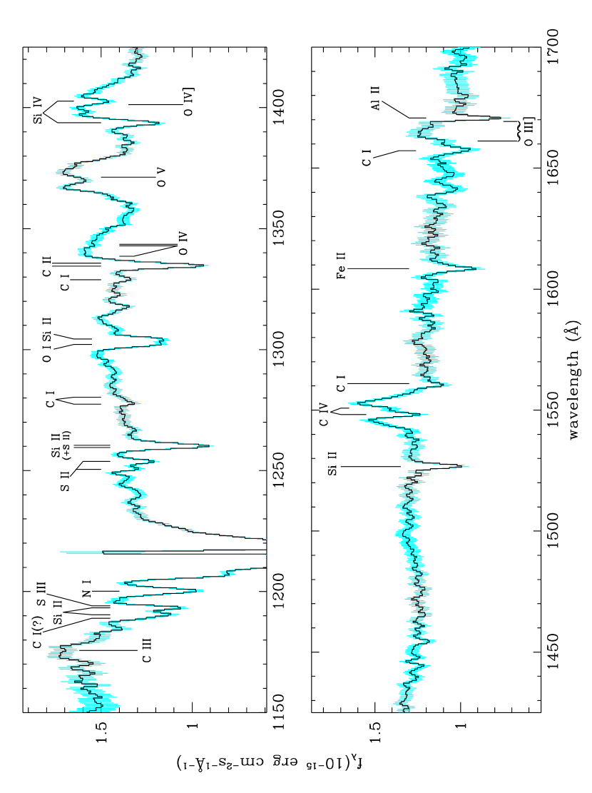
Figure 1: Far-UV spectrum of 4U 1626-67 (=KZ TrA) from a total exposure of 31.2 ks with HST/STIS. No correction for the small reddening of this object has been made, but to aid clarity 3 pixel boxcar smoothing has been applied. Numerous emission and absorption lines are present, the most significant of which have been labelled. Emission lines are labelled from beneath, whilst absorption or coinciding emission/absorption lines are labelled from above. Note in particular the broad and complicated emission profiles; these are discussed further in the text.

2 OBSERVATIONS AND DATA REDUCTION

We obtained HST/STIS UV observations of 4U 1626-67 on 1999 April 2, May 31 and June 1 totaling 12 HST orbits; we also extracted a further 4 orbits of archival data taken a year earlier on 1998 April 23 as part of another program. All data were taken with either the low resolution G140L (FUV) or G230L (NUV) gratings, which give useful wavelength ranges of $\sim$1160–1700Å and $\sim$1700–3150Å, at 1.2Å and 3.2Å resolutions respectively. The FUV and NUV MAMA detectors were operated in Time-Tag mode, which is then effectively photon-counting. All these data were reduced by the On-The-Fly Reprocessing system at STScI, which utilizes the best currently available calibration files, software and data parameters. The products provided include 2-D spectral images created by accumulating the photon event list over the exposure during a given HST orbit, as well as the wavelength and flux-calibrated 1-D spectra extracted from these. We then also applied additional wavelength corrections using the STSDAS WAVECAL routine (if not previously completed), which makes use of the wavelength calibration (arc) spectra taken with each science exposure. Lastly, we derived a fully time-averaged spectra in each band from all the data (weighting each HST orbit’s data according to exposure time), which amounts to total exposure times of 31.2 ks (8.7 hrs) in the FUV (and 10.8 ks in the NUV).

3 DATA ANALYSIS AND RESULTS

In figure 1 we present the complete FUV spectrum (not corrected for the small reddening towards this object), with 3 pixel boxcar smoothing applied to aid clarity (and with 1$\sigma$ error-bars combined accordingly). The long exposure provides good signal-to-noise, and numerous prominent broad emission lines and narrower absorption features stand out. By contrast, the NUV spectrum shows no very strong emission features and only absorption lines (from Mg II, Mn II, Fe II and Zn II) of strength consistent with interstellar origin; hence we will only make occasional further reference to results from this NUV spectrum in the remainder of this paper.

Apart from the very strong absorption feature at $\sim$1215Å due to Ly$\alpha$, which has prominent damping wings, the results of Gaussian fits (using the full-resolution data) to all the prominent FUV lines (measured line centers, FWHM and equivalent widths) are presented in table 1. Almost all of the emission lines exhibit complex structures and in most cases emission and absorption lines coincide. We will discuss the fits to these more complex profiles in turn, in the following sections. For the remaining absorption lines we fit each line with a single Gaussian, with center, width and normalization as free parameters. In the case of blends, if the separation of the two (or more) lines was greater than the spectral resolution, we included a Gaussian profile for each.

Similarly for each line contributing to the emission/absorption line complexes we used unconstrained Gaussians. However, for the components of multiplets additional constraints were applied. We required the ratio of the components’ centers (effectively the spacing) to agree with that of the vacuum wavelengths, and the FWHM of each component to be the same. The absorption components are likely dominated by interstellar absorption. Hence we left the ratio of the fluxes (e.g. the doublet ratio) free to allow for the probable range of optical depth for the absorbing clouds. However, attempts at leaving the ratios free for the emission too, indicated that the data are insufficient to meaningfully constrain these values, and often actually produced unphysical results. Hence, in most cases we simply assumed the optically thick limit for the emission lines and used the appropriate relative intensities as tabulated in the National Institute of Standards and Technology (NIST) listings. Most observational determinations, as well as the results of modeling, (see e.g. Ko & Kallman, 1994), indicate that these resonant emission lines are typically optically thick. Nevertheless, for the Si IV and C IV doublets we also examined the optically thin limit (where the doublet ratio is 2:1 for the lower to higher wavelength components), but found no substantive differences (see the relevant section for details). We therefore tabulate (and show figures) based on the optically thick assumption. Lastly, we also tried twin-Gaussians to represent two separate blue- and red-shifted emission regions, i.e. as was done for the double-peaked X-ray lines by SCH01.

Table 1: Parameters of Gaussian fits to FUV absorption and emission lines in 4U 1626-67

Compo	ID	$\lambda_{vac}$	$\Delta\lambda$	$V$	FWHM	Flux ($10^{-16}$	EW
-nent			(Å)	( $\hbox{km}\thinspace\hbox{s}^{-1}$)	( $\hbox{km}\thinspace\hbox{s}^{-1}$)	$\hbox{erg}\thinspace\hbox{cm}^{-2}\thinspace\hbox{s}^{-1}$)	(Å)
+	C III	1175.64	$-0.33\pm 0.52$	$-85\pm 135$	$1440\pm 330$	$10.6\pm 3.4$	$0.68\pm 0.22$
–	C I(?)	1188.99	$-0.11\pm 0.25$	$-30\pm 65$	$380\pm 150$	$-3.9\pm 1.6$	$0.26\pm 0.11$
–	Si II	1190.42	$0.25\pm 0.11$	+$65\pm 30$	$360\pm 70$	$-6.5\pm 1.4$	$0.45\pm 0.10$
–	Si II	1193.29	$-0.01\pm 0.06$	0$-5\pm 15$	$470\pm 40$	$-9.2\pm 1.0$	$0.63\pm 0.07$
–	+S III	1194.06	$-0.78\pm 0.06$	$-195\pm 15$
–	N I	1200.13	$0.16\pm 0.06$	+$40\pm 15$	$610\pm 40$	$-12.3\pm 1.0$	$0.88\pm 0.07$
–	S II	1250.58	$-0.98\pm 0.40$	$-235\pm 95$	$850\pm 230$	$-10.5\pm 2.8$	$0.76\pm 0.20$
–	S II	1253.81	$-0.02\pm 0.11$	+$-5\pm 25$	$460\pm 90$	$-5.9\pm 1.3$	$0.42\pm 0.09$
–	Si II	1260.42	$-0.28\pm 0.05$	$-65\pm 10$	$560\pm 30$	$-12.6\pm 0.9$	$0.93\pm 0.07$
–	(+S II)	1259.52	$0.62\pm 0.05$	+$150\pm 10$
–	C I	1277.41	$0.33\pm 0.21$	+$75\pm 50$	$320\pm 110$	$-1.9\pm 0.8$	$0.13\pm 0.06$
–	C I	1280.33	$-0.54\pm 0.80$	$-125\pm 190$	$380\pm 280$	$-1.2\pm 1.0$	$0.09\pm 0.07$
–	O I	1302.17	$0.04\pm 0.14$	$10\pm 30$	$600\pm 110$	$-12.0\pm 2.7$	$0.81\pm 0.19$
–	Si II	1304.37	$0.14\pm 0.11$	$30\pm 25$	$390\pm 70$	$-6.8\pm 1.9$	$0.46\pm 0.13$
–	C I	1328.83	$0.44\pm 0.23$	$100\pm 50$	$530\pm 170$	$-2.9\pm 1.0$	$0.20\pm 0.07$
–	C II	1334.53	$-0.01\pm 0.16$	+$0\pm 35$	$500\pm 50$	$-12.0\pm 1.9$	$0.85\pm 0.14$
–	C II	1335.71	$-0.01\pm 0.16$	+$0\pm 35$	$500\pm 50$	$-4.6\pm 2.4$	$0.32\pm 0.17$
+	O IV	1338.61	$0.37\pm 0.47$	0$85\pm 105$	$2780\pm 380$	0+$9.7\pm 1.4$	$0.69\pm 0.10$
+	O IV	1342.99	$0.37\pm 0.47$	0$85\pm 105$	$2780\pm 380$	0+$6.5\pm 1.0$	$0.43\pm 0.07$
+	O IV	1343.51	$0.37\pm 0.47$	0$85\pm 105$	$2780\pm 380$	0+$9.1\pm 1.4$	$0.66\pm 0.10$
–	C I	1328.83	$0.30\pm 0.18$	+$70\pm 40$	$440\pm 100$	$-2.2\pm 0.7$	$0.15\pm 0.05$
–	C II	1334.53	$-0.21\pm 0.20$	$-45\pm 45$	$400\pm 70$	$-9.1\pm 1.9$	$0.64\pm 0.13$
–	C II	1335.71	$-0.21\pm 0.20$	$-45\pm 45$	$400\pm 70$	$-6.6\pm 3.0$	$0.47\pm 0.21$
+b∗	O IV	1338.61	$-3.61\pm 0.38$	$-805\pm 85$	$770\pm 230$	0+$2.5\pm 0.9$	$0.18\pm 0.07$
+b∗	O IV	1342.99	$-3.61\pm 0.38$	$-805\pm 85$	$770\pm 230$	0+$1.6\pm 0.6$	$0.11\pm 0.04$
+b∗	O IV	1343.51	$-3.61\pm 0.38$	$-805\pm 85$	$770\pm 230$	0+$2.9\pm 1.1$	$0.21\pm 0.08$
+r∗	O IV	1338.61	$2.88\pm 0.77$	+$645\pm 170$	$1850\pm 430$	0+$6.2\pm 1.6$	$0.44\pm 0.11$
+r∗	O IV	1342.99	$2.88\pm 0.77$	+$645\pm 170$	$1850\pm 430$	0+$4.0\pm 1.0$	$0.27\pm 0.07$
+r∗	O IV	1343.51	$2.88\pm 0.77$	+$645\pm 170$	$1850\pm 430$	0+$7.1\pm 1.8$	$0.52\pm 0.13$
+	O V	1371.29	$0.27\pm 0.31$	+$60\pm 70$	$2820\pm 190$	$49.1\pm 4.3$	$3.66\pm 0.32$
+b∗	O V	1371.29	$-4.49\pm 0.22$	$-980\pm 50$	$950\pm 150$	$14.2\pm 2.6$	$1.04\pm 0.19$
+r∗	O V	1371.29	$2.75\pm 0.30$	+$600\pm 65$	$1680\pm 150$	$28.9\pm 3.0$	$2.12\pm 0.22$
+	O V	1371.29	$0.20\pm 0.18$	+$45\pm 40$	$1690\pm 70$	+.$491\pm 20$	$36.1\pm 1.5$
–	O V	1371.29	$-0.21\pm 0.19$	$-45\pm 40$	$1610\pm 80$	$-447\pm 21$	$32.9\pm 1.6$
+	Si IV	1393.76	($\lambda$ fixed)	—	$850\pm 460$	$12.5\pm 12.2$	$0.93\pm 0.91$
–	Si IV	1393.76	($\lambda$ fixed)	—	$590\pm 130$	$-18.4\pm 8.0$	$1.36\pm 0.59$
+	O IV]	1401.35	($\lambda$ fixed)	—	$3060\pm 180$	$42.5\pm 4.5$	$3.17\pm 0.34$
+	Si IV	1402.77	($\lambda$ fixed)	—	$840\pm 450$	$10.1\pm 9.9$	$0.76\pm 0.74$
–	Si IV	1402.77	($\lambda$ fixed)	—	$590\pm 130$	$-12.0\pm 5.2$	$0.90\pm 0.39$
+	Si IV	1393.76	$2.79\pm 0.37$	$600\pm 80$	$2000\pm 160$	$24.3\pm 2.8$	$1.81\pm 0.21$
–	Si IV	1393.76	$-0.02\pm 0.08$	$-5\pm 15$	$520\pm 50$	$-10.3\pm 1.2$	$0.76\pm 0.09$
+	O IV]	1401.35	$1.52\pm 0.27$	$325\pm 60$	$680\pm 10$	$13.4\pm 8.4$	$1.00\pm 0.63$
+	Si IV	1402.77	$2.81\pm 0.37$	$600\pm 80$	$1990\pm 160$	$19.4\pm 3.7$	$1.46\pm 0.28$
–	Si IV	1402.77	$-0.02\pm 0.08$	$-5\pm 15$	$520\pm 50$	$-13.8\pm 1.3$	$1.03\pm 0.10$
+∗	Si IV	1393.76	$-0.55$	$-120$	$870$	$13.2$	$0.97$
–∗	Si IV	1393.76	$-0.23$	$-50$	$540$	$-13.9$	$1.04$
+b∗	O IV]	1401.35	$-3.77$	$-805$	$770$	+0$8.8$	$0.65$
+r∗	O IV]	1401.35	$3.00$	+$645$	$1850$	$21.6$	$1.63$
+∗	Si IV	1402.77	$-0.55$	$-120$	$870$	$10.5$	$0.79$
–∗	Si IV	1402.77	$-0.23$	$-50$	$540$	$-9.5$	$0.71$
–	Si II	1526.71	$0.11\pm 0.07$	$20\pm 14$	$380\pm 30$	$-7.2\pm 0.8$	$0.56\pm 0.06$
+	C IV	1548.20	$0.26\pm 0.15$	$50\pm 30$	$1490\pm 120$	$27.5\pm 5.2$	$2.20\pm 0.42$
–	C IV	1548.20	$-0.02\pm 0.07$	$-5\pm 15$	$430\pm 40$	$-14.2\pm 1.9$	$1.14\pm 0.15$
+	C IV	1550.77	$0.26\pm 0.15$	$50\pm 30$	$1490\pm 120$	$24.8\pm 4.7$	$1.98\pm 0.37$
–	C IV	1550.77	$-0.02\pm 0.07$	$-5\pm 15$	$430\pm 40$	$-9.9\pm 1.8$	$0.79\pm 0.14$
–	C I	1560.91	$-0.46\pm 0.17$	$-90\pm 35$	$320\pm 90$	$-3.1\pm 1.0$	$0.25\pm 0.08$
–	Fe II	1608.45	$0.00\pm 0.13$	+$0\pm 25$	$330\pm 80$	$-5.9\pm 1.6$	$0.51\pm 0.13$
–	C I	1657.22	$0.40\pm 0.20$	$70\pm 35$	$260\pm 90$	$-2.5\pm 1.1$	$0.23\pm 0.10$
+	O III]	1661.20–	$0.60\pm 0.30$	$110\pm 55$	0$580\pm 110$	$17.1\pm 4.6$	$1.63\pm 0.44$
	(7 comps)	–1669.30
–	Al II	1670.79	$-0.24\pm 0.07$	$-45\pm 15$	$280\pm 30$	$-9.5\pm 1.5$	$0.91\pm 0.15$

Note. — The entries in the table are grouped (separated by horizontal spaces) according to which lines were blended together and therefore required simultaneous fitting.

3.1 Fits to individual Emission/Absorption line complexes

3.1.1 C III $\lambda 1176$

This profile appears to be flat topped, or even double-peaked. However, given the lower signal-to-noise at this short wavelength end of the spectral range, such details are well within the uncertainties and a simple single Gaussian fit is as appropriate as any more complex model. The resulting line center is consistent within the uncertainties with the weighted average of the vacuum wavelengths of the closely spaced multiplet components.

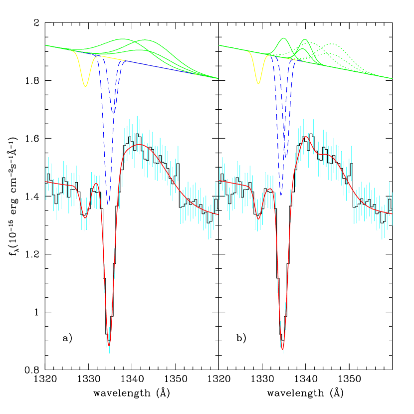
Figure 2: Gaussian line profile fits to O IV triplet $\lambda 1342$ emission, with absorption lines of C I $\lambda 1329$ (solid line) and the C II $\lambda$1335, $\lambda$1336 doublet (dashed). a) Single emission component for each of the O IV triplet lines, note the very broad profile required (FWHM=2800 $\hbox{km}\thinspace\hbox{s}^{-1}$). b) Assuming blue- (solid) and red-shifted (dotted) components for each triplet line provides a marginally better fit, but with significantly broader red-shifted than blue-shifted lines.

3.1.2 O IV triplet $\lambda 1342$

In addition to the three emission components of the O IV triplet, one must also include absorption lines of C I $\lambda 1329$ and the C II $\lambda$1335, $\lambda$1336 doublet in order to fit the observed profile. Even with the 1000 $\hbox{km}\thinspace\hbox{s}^{-1}$ span of the three components of the multiplet, the breadth of this emission feature requires a very large FWHM of 2800 $\hbox{km}\thinspace\hbox{s}^{-1}$ for each separate component (see fig. 2a). A better representation may well be a two Gaussian double-peaked profile for each component, as was used for the SCH01 X-ray line spectra. This more complex model does provide a better fit (fig. 2b), with a broad (FWHM=800 $\hbox{km}\thinspace\hbox{s}^{-1}$) blue-shifted component ($V=-800$ $\hbox{km}\thinspace\hbox{s}^{-1}$), but an even broader (FWHM=1900 $\hbox{km}\thinspace\hbox{s}^{-1}$) red-shifted component ($V=600$ $\hbox{km}\thinspace\hbox{s}^{-1}$).

3.1.3 O V $\lambda 1371$

This singlet line, unaffected by any expected strong interstellar absorption lines should be the most clear cut case. However, the single Gaussian fit again yields a very large FWHM of $2800\thinspace\hbox{$\hbox{km}\thinspace\hbox{s}^{-1}$}$, as well as being clearly a very poor fit (see fig. 3a). Once again motivated by the double-peaked X-ray lines, we have attempted such a fit, which works well (see fig. 3b). This yields velocity shifts of –950 $\hbox{km}\thinspace\hbox{s}^{-1}$and 650 $\hbox{km}\thinspace\hbox{s}^{-1}$for the blue- and red-shifted components respectively, with reduced, but like O IV $\lambda$1342, differing FWHM of 950 and 1700  $\hbox{km}\thinspace\hbox{s}^{-1}$. For a disk representation the FWHM should be the same; hence this implies that there may be additional red-shifted emission contributions. A fit using one blue-shifted and two red-shifted Gaussian components is also possible with a similar significance.

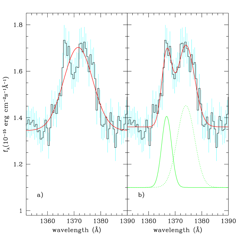
Figure 3: Gaussian line profile fits to O V $\lambda 1371$. a) With a single emission component a very broad line is required, but this is a noticeably poor fit due to the dip at $\sim$1369Å, b) double-peaked emission, with red-shifted component (dotted line) much broader than the blue (solid), providing a much better fit.

Our attempt to fit the profile with a single emission peak and absorption to account for the dip at $\sim$1369Å failed, although it is still possible that in addition to multiple emission peaks there is some absorption. For instance, phase-resolved STIS FUV spectroscopy of Her X-1 (Vrtilek et al., 2001; Boroson et al., 2000) also revealed unusual features in the O V line profile. In addition to the broad and narrow emission components, absorption was required for the fits in Her X-1, which moved in phase with the binary and therefore was interpreted as a local effect. We note that published STIS FUV spectra (phased-averaged) of the X-ray transient XTE J1859+226 (Haswell et al., 2002) also shows a similar O V structure to 4U 1626-67, but these authors do not discuss the profile.

3.1.4 Si IV $\lambda$1394, $\lambda$1403 doublet + O IV] $\lambda 1401$ blend

This is the most complex of the emission/absorption profiles in our spectrum. Our most basic model is to assume broad emission components for each of the Si IV doublet lines and the O IV line and narrower interstellar Si IV absorption, with the doublet ratio (DR) constrained to the optically thick case (=1.25). We first tried the model fixing all the central wavelengths to their vacuum values, and then relaxed this constraint. In this instance, significant differences in the line parameters resulted. Although, in both cases the model can be made to fit the profile quite well (apart from failing to delineate the drop in flux between the two Si IV lines at $\sim$1398Å), physical consideration of the resulting parameters shows them to be questionable. The fits favor large line fluxes in both the emission and absorption components, which then balance out to provide the profile required. In the fully constrained fit almost all the emission flux comes from a very strong (EW=680 $\hbox{km}\thinspace\hbox{s}^{-1}$) and very broad (FWHM=3000 $\hbox{km}\thinspace\hbox{s}^{-1}$) O IV] line (see fig. 4a), whilst in the less constrained fit a large 600 $\hbox{km}\thinspace\hbox{s}^{-1}$ velocity shift of the Si IV doublet is found, together with very high fluxes and 2000 $\hbox{km}\thinspace\hbox{s}^{-1}$ line widths (see fig. 4b). Using a DR of 2 for the optically thin limit had little effect apart from the absorption intensities adjusting to a similar ratio to balance the emission once again. Clearly much more complex emission components are needed. Since there is evidence that O V and possibly O IV profiles are better fit by an asymmetric twin-Gaussian model, we have tested whether such an O IV profile can fit the semi-forbidden line here. We have constrained the components to have the same velocity shifts, widths and relative normalizations as O IV $\lambda$1342, and find that this does work reasonably well (see fig. 4c). We note, however, that a similar double-peaked profile would be too broad to fit the superimposed Si IV features as they are relatively narrow.

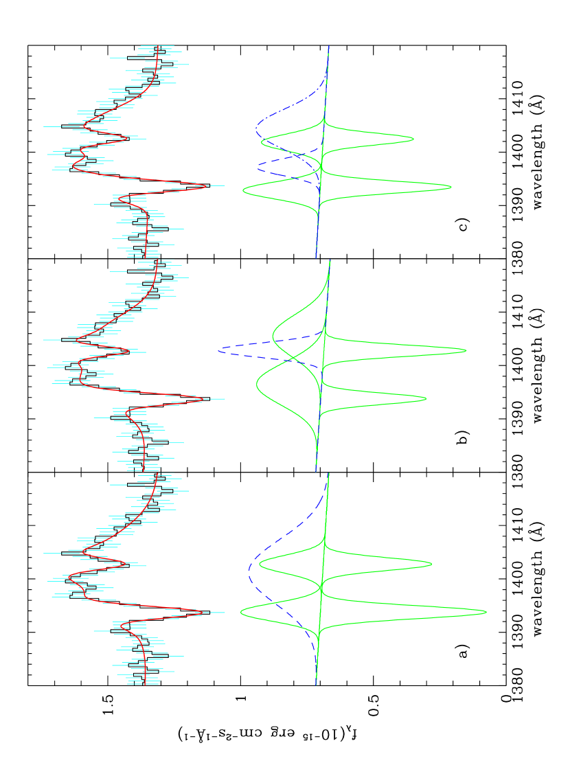
Figure 4: Gaussian line profile fits to the complex Si IV $\lambda$1394, $\lambda$1403 doublet (solid lines) + O IV] $\lambda 1401$ (dashed) blend. Both emission and absorption components are included for the Si IV doublet lines. a) Constrained fit with line centers given by vacuum wavelengths. This results in broad and strong O IV] emission, with narrow Si IV emission, balancing only slightly narrower absorption lines. b) With the line centers now unconstrained (apart from the separation of the doublet components), the fit yields much broader Si IV emission redshifted by as much as 600 $\hbox{km}\thinspace\hbox{s}^{-1}$, and narrow O IV] shifted to balance the Si IV $\lambda$1403 absorption in an unlikely manner. c) Motivated by the fits to O IV $\lambda$1371 and O V $\lambda$1342, the single O IV] line has been replaced with a twin-Gaussian profile (dashed and dot-dashed), with separation, FWHM and relative normalizations constrained to that found for O IV $\lambda$1342. Essentially the results are similar to a), though the Si IV emission is now slightly blue-shifted relative to its absorption. None of these fits is physically very satisfying, and in all likelihood the true underlying emission profiles are even more complex.

3.1.5 C IV doublet $\lambda 1549$

As the baseline model for this doublet structure we assume the presence of the two doublet emission lines (with DR=1.11 for optically thick limit) and corresponding doublet absorption lines, together with absorption at 1561Å, which we attribute to C I. As can been seen in figure 5, this model does provide a reasonable fit to the data, with only a small 50 $\hbox{km}\thinspace\hbox{s}^{-1}$ shift (comparable to the uncertainty) in the emission doublet wavelength required. The strong C IV emission is a common feature of LMXB FUV spectra, but the absorption is unusually pronounced. Checking the optically thin limit for the emission (with DR=2), we found that the absorption strengths are in fact insensitive to this ratio. Even trying double-peaked emission for each component of emission doublet cannot reduce the depth of the absorption lines required, since the shape of the line profiles constrains each emission component to be almost as broad as the single Gaussians shown. We will discuss the strong C IV absorption and the probable C I absorption further in §§ 4.1.1. Also, we note that the width/velocity spread of the emission lines is only about half that of the O V and O IV.

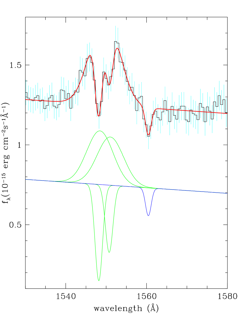
Figure 5: Gaussian line profile fit to C IV doublet $\lambda 1549$, including both emission and absorption, together with probable C I $\lambda$1561 absorption. Fairly broad (FWHM=1500 $\hbox{km}\thinspace\hbox{s}^{-1}$) and strong C IV is required, with much narrower (FWHM=430 $\hbox{km}\thinspace\hbox{s}^{-1}$) absorption.

3.1.6 O III] multiplet $\lambda 1661-1669$

This profile can be adequately fit with a single emission Gaussian for each of the multiplet components, together with Al II $\lambda 1671$ and yet more C I ($\lambda 1657$) absorption. But, as for the O IV $\lambda$1342 and O V $\lambda$1371 lines, a very large FWHM$\sim$2800 $\hbox{km}\thinspace\hbox{s}^{-1}$ is indicated for each component by the fit, and the feature is overall unusually strong for an LMXB, as compared to, for instance, the Si and C doublets.

4 DISCUSSION

4.1 Absorption and emission strengths and the local elemental abundances

Henceforth, in the cases of the complex emission and absorption profiles, we only consider the fluxes/EWs given by the physically reasonable fits. These particular fits are indicated by asterisks in table 1 to aid cross-reference.

4.1.1 Interstellar versus local absorption

At first glance, the equivalent widths (EWs) of the many absorption lines (if interstellar in origin) would appear rather large given the low column towards this source, $E(B-V)=0.11\pm 0.1$ (SCH01). However, consideration of the results from the HST Quasar Absorption Line Key Project suggests otherwise for most of the lines. Savage et al. (2000) report on the Galactic interstellar features they identified in the spectra of this large sample of 83 quasars. Their sample includes a range of $E(B-V)$ from 0.014 to 0.155, as determined from radio H I measurements; therefore the range encompasses the reddening of 4U 1626-67. In table 2 we summarize our measured equivalent widths for the numerous absorption lines (including those superimposed on top of emission), and present the comparative results from Savage et al. (2000), both their tabulated median and rms values for the EWs and an estimate of the maximum they measured (from their fig. 5). In almost all cases where a comparison is possible, our measured values for 4U 1626-67 lie comfortably within the range for the quasars. The only exceptions are the Si IV $\lambda$1393/1402, C II $\lambda$1335/1336 and C IV $\lambda$1548/1550. As noted above the Si IV $\lambda$1394/1403 lines are blended with O IV] making fitting to this profile rather uncertain. Given the fact that the other Si lines (all Si II) have EWs comparable to typical interstellar absorption might suggest that the large Si IV EWs are an artefact of poor fitting and/or simply the use of too simplified a model. However, for C the situation is different, even ignoring the complicated C IV doublet. The C II blend is too deep, though just consistent with the maximum interstellar EW value, and we also identified a number of C I absorption lines in our spectrum, of which only C I $\lambda$1329 is normally seen (see e.g. Morton et al., 1972). In the case of C IV even trying double-peaked emission had very little effect on the amount of absorption required, and here the excess is large. The most likely explanation would seem to be excess C, at various ionization stages, local to the system. Indeed, SCH01 found that fits to their X-ray spectra were improved by including the effects of a carbon $K$ edge with an overabundance of C relative to H of $(5-18)\times$ solar.

Table 2: Comparison of 4U 1626-67 Absorption line EWs to Interstellar lines from HST Quasar Key Project

ID	$\lambda_{vac}$	Flux ($10^{-16}$	EW	EW from HST Key Project
	(Å)	$\hbox{erg}\thinspace\hbox{cm}^{-2}\thinspace\hbox{s}^{-1}$)	( $\hbox{km}\thinspace\hbox{s}^{-1}$)	Median ( $\hbox{km}\thinspace\hbox{s}^{-1}$)	Maximum ( $\hbox{km}\thinspace\hbox{s}^{-1}$)
C I(?)	1188.99	$-3.88\pm 1.61$	$67\pm 28$	0–	–
Si II	1190.42	$-6.53\pm 1.39$	$113\pm 24$	0–	–
Si II	1193.29	$-9.20\pm 0.97$	$159\pm 17$	0–	–
S III	1194.06	$-9.20\pm 0.97$	$159\pm 17$	0–	–
N I	1200.13	$-12.28\pm 0.99$	$219\pm 18$	$240\pm 65$	260
S II	1250.58	$-10.49\pm 2.80$	$182\pm 49$	0–	–
S II	1253.81	$-5.91\pm 1.32$	$101\pm 23$	0$70\pm 90$	220
Si II	1260.42	$-12.63\pm 0.94$	$221\pm 18$	$190\pm 65$	320
(+S II)	1259.52
C I	1277.41	$-1.89\pm 0.79$	$31\pm 13$	0–	–
C I	1280.33	$-1.21\pm 0.99$	$20\pm 16$	0–	–
O I	1302.17	$-11.99\pm 2.73$	$187\pm 43$	$105\pm 55$	220
Si II	1304.37	$-6.84\pm 1.86$	$106\pm 29$	0$95\pm 35$	190
C I	1328.83	$-2.88\pm 1.03$	$46\pm 16$	0–	–
C II	1334.53	$-16.59\pm 3.10$	$260\pm 50$	$160\pm 45$	230
+C II	1335.71
Si IV	1393.76	$-10.25\pm 1.17$	$163\pm 19$	0$60\pm 40$	160
Si IV	1402.77	$-13.81\pm 1.32$	$220\pm 21$	0$40\pm 10$	60
Si II	1526.71	$-7.17\pm 0.79$	$109\pm 12$	0$95\pm 25$	150
C IV	1548.20	$-14.21\pm 1.91$	$220\pm 30$	0$80\pm 25$	110
C IV	1550.77	$-9.92\pm 1.79$	$153\pm 28$	0$45\pm 20$	80
Fe II	1608.45	$-5.87\pm 1.56$	$94\pm 25$	0–	–
C I	1657.22	$-2.51\pm 1.09$	$42\pm 18$	0–	–
Al II	1670.79	$-9.48\pm 1.52$	$164\pm 26$	$115\pm 30$	220

4.1.2 Emission line strengths

Once we have taken into account the pronounced absorption for both the Si IV/O IV] blend and C IV with our Gaussian fitting, these emission features turn out to be the strongest, both with EW$\sim$4Å. The various O emission lines are also generally prominent, the more typical lines of O V and O IV having EW$\sim$3 and 2Å respectively, whilst even the unusual O III] feature yields $\sim$1.5Å. The weakest line we measure is that of C III with only $\sim$0.5Å. We note that both N V$\lambda$1240 and He II$\lambda$1640, common in a large variety of high excitation objects, are very weak or entirely absent in our spectrum of 4U 1626-67.

We also compare our results on the emission line strengths of 4U 1626-67 with those published for Her X-1 (Anderson et al., 1994; Boroson et al., 1996), Sco X-1 (Kallman et al., 1998), and XTE J1859+226 and XTE J1118+480 (Haswell et al., 2002) based on other HST data. These systems represent respectively, an intermediate mass X-ray pulsar, the “prototypical” LMXB, and two rather different soft-X-ray transients (black-hole candidates) in outburst; hence they should provide a reasonably diverse context for our study.

Common emission line characteristics of these comparison objects include: (i) very prominent N V $\lambda$1238, 1242 doublet, (ii) equally strong or stronger C IV $\lambda$1548, $\lambda$1550 doublet (except for XTE J1118+480, for which abundance anomalies are postulated), (iii) prominent He II$\lambda$1641 , (iv) similar strength Si IV/O IV] blend, and (v) usually slightly weaker O V and C III$\lambda$1175 (again except for XTE J1118+480). Hence, the absence of noticeable N V and He II is one distinctly unusual feature of 4U 1626-67. The lack of He II provides strong support for the conclusion of the X-ray abundance analysis of SCH01, namely that the white dwarf has no He to transfer, but is in fact the core of a more massive initial star, comprised largely of either C-O-Ne or O-Ne-Mg. The apparent reduction in N abundance is then not unexpected. Furthermore, it also appears that there is an excess of O in 4U 1626-67; O IV$\lambda$1342 is very strong here whereas it is only otherwise noted in the case of Sco X-1 (although it may also be present in the published spectrum of XTE J1859+226), whilst O III] multiplet $\lambda 1661-1669$ is not identified in any of these comparison systems.

In terms of distinguishing between the two possible white dwarf compositions, Mg is the key. As SCH01 discuss, either C-O-Ne or O-Ne-Mg white dwarf models can account for the high observed Ne and C abundances. In the FUV the only Mg interstellar absorption line that is sometimes seen is Mg II at 1240Å  but in the NUV there is the Mg II $\lambda$2796, $\lambda$2803 doublet, which again appears as an interstellar absorption feature but is also found in emission in a range of astrophysical situations, including quiescent LMXBs (McClintock & Remillard, 2000). It is possible that there is weak $\lambda$1240 absorption, whilst analysis of the $\lambda$2796, $\lambda$2803 doublet (in our NUV spectrum), is rather complex and inconclusive. The lower spectral resolution of the NUV spectrum makes any disentangling of emission versus absorption components difficult. There is marginal evidence for emission, which would in turn imply probable excess absorption, but equally if we assume no emission the absorption is comparable to what we would expect from interstellar. It would seem that further higher signal-to-noise/resolution spectra concentrating on this Mg II doublet would be helpful to derive observational constraints from this avenue.

4.2 Emission region dynamics and location

In terms of the emission line profiles we find two broad categories from our fitting; those consistent with a single emission region and those preferring a Doppler pair of emission regions. C III and C IV can be represented by emission from a single region with a broad dispersion in velocities giving a FWHM$\sim$1500 $\hbox{km}\thinspace\hbox{s}^{-1}$ for the lines, with a negligible shift in line centers. Si IV is similar (considering the final fit with double-peaked O IV]), as is O III], although the FWHM$\sim$900 $\hbox{km}\thinspace\hbox{s}^{-1}$ and 600 $\hbox{km}\thinspace\hbox{s}^{-1}$ are somewhat smaller and 100 $\hbox{km}\thinspace\hbox{s}^{-1}$ velocity shifts were indicated, though for O III] and possibly for Si IV these may well not be significant. By contrast, the more highly ionized O V singlet most likely requires a Doppler pair of emission regions (with $V\sim-1000$ and +600 $\hbox{km}\thinspace\hbox{s}^{-1}$), and similar results are suggested for the O IV triplet. Even then the red-shifted components have very large FWHM$\sim$2000 $\hbox{km}\thinspace\hbox{s}^{-1}$, roughly twice that of the blue-shifted components, which may indicate that the there are in fact multiple red-shifted emission regions.

Detailed modeling of the various emission regions and their dynamics is beyond the scope of this paper. However, some physical insights can be gained by considering results from earlier general studies of UV line formation. It should be noted that all these studies assumed typical cosmic abundances for the emitting gas, in particular that the heavier elements have trace abundances relative to H and He, which is almost certainly not the case for the transferred material in 4U 1626-67.

Kallman & McCray (1982) presented a range of theoretical models for the ionization structure of gas irradiated by a powerful X-ray source, covering a range of astrophysically relevant parameters. This enables us to look at the differing dependence of the various ionic species on the ionization parameter ($\xi=L_{X}/nR^{2}$, where $L_{X}$ is the X-ray irradiating luminosity, $n$ is the gas density and $R$ is the distance from the emission region to the X-ray source). Their 8 models include different values of the luminosity, its spectral shape and the gas density. The case of a high density gas ($n=10^{11}{\rm cm}^{-3}$), illuminated by a 10 keV thermal bremsstrahlung X-ray spectrum with $L_{X}=10^{37}$ $\hbox{erg}\thinspace\hbox{s}^{-1}$with line trapping effects included, is particularly interesting. Such conditions may well be similar to those in an accretion disc corona/atmosphere above the disc of 4U 1626-67. The calculations show that the peak of the predicted abundances for our two groups of emission lines are separated in terms of the value of $\xi$ required. C III, Si IV and O III all peak at around $\log\xi=1.35$, whereas O IV and  V require a significantly higher $\log\xi\sim 1.65$. C IV lies between the two in terms of $\xi$, but still its abundance is negligible by the time you reach the peak $\log\xi$ value for the more highly ionized O species. Although the details will not be exactly applicable to our case, the important point is that such a division in terms of the values of $\xi$ is plausible. In consequence, there could be differences in the radial dependence of the emission. For instance, modeling of the broad emission lines of Her X-1 (admittedly for a posited disk wind situation) by Chiang (2001) found that the outer radii of the emission region for a given ion were systematically smaller for the higher ionization lines. Similar “ionization stratification” was also found from reverberation mapping of the broad line regions of AGNs (see e.g. Krolik et al., 1991; Korista et al., 1995). The effect is probably quite subtle, and in fact specific modeling of the emission lines from X-ray heated accretion discs by Ko & Kallman (1994) did not find any clear difference in the radial dependence of the line formation between C IV and O V, although for Si IV the contributions did drop more rapidly with decreasing radial location. They also predicted that overall the greatest contributions to the UV lines should be from the outermost radii.

Observationally, the trend in $\xi$ does appear to follow that of the velocity spread/FWHM of our emission lines. For double-peaked emission lines the velocity shift of the peaks should be a measure of the Keplerian velocity of the outermost contributing radial annulus (see Smak, 1981; Horne & Marsh, 1986), whilst for apparently single-peaked lines the HWHM should also be an approximate indicator. We note that both the single Gaussian and the twin-Gaussian profiles are merely different approximations to the actual velocity profile one would expect from gas distributed in a Keplerian flow. In fact, the separation into the two groups is probably a consequence of which is the better approximation for a given velocity spread.

To aid in the comparison of observations with the above models we may also consider the even broader X-ray lines. SCH01 found that all these lines had similar overall width, and hence could be fitted with double-peaked profiles. In their case, the FWHM of the blue and red-shifted components could be taken as equal at $\sim$2000–3000 $\hbox{km}\thinspace\hbox{s}^{-1}$, with large velocity shifts for peaks ranging from –1600 $\hbox{km}\thinspace\hbox{s}^{-1}$ to –2600 $\hbox{km}\thinspace\hbox{s}^{-1}$ in the blue and 800–1900 $\hbox{km}\thinspace\hbox{s}^{-1}$ in the red. As they comment, these line profiles could also be consistent with a disc origin. If one considers the velocities of the various X-ray and FUV lines in terms of a Keplerian accretion disc or atmosphere just above (assuming $i=30^{\circ}$, the upper limit for a 0.02 $M_{\odot}$donor), one would place the outermost contributing radii for C III, Si IV and O III at the outer (tidally truncated) edge ($r_{t}\simeq 2\times 10^{10}$cm, where $V\sin i=530$ $\hbox{km}\thinspace\hbox{s}^{-1}$), C IV a little farther in, O IV and O V slightly farther in still and for the X-ray lines from $r\simeq 3\times 10^{10}$cm to the inner edge (at magnetospheric corotation, $r_{co}=6.5\times 10^{8}$ cm, where $V\sin i=2900$ $\hbox{km}\thinspace\hbox{s}^{-1}$). But this is where the simple physical picture outlined above appears to break down. As discussed by SCH01, given the luminosity of the source ($L_{X}=2\times 10^{36}(d/3{\rm kpc})^{2}\thinspace\hbox{$\hbox{erg}\thinspace\hbox{s}^{-1}$}$), and a gas density of $n\sim 10^{11}$cm^-3 requires $R\mbox{${}^{>}\mskip-10.5mu_{\sim}$}10^{10}(d/3{\rm kpc})$, comparable to the radius of the outer disc to obtain $\xi<10^{3}$ erg cm s^-1 and allow formation of even the more highly ionized X-ray line emitting species. For our FUV lines, with $\xi\sim 50$ erg cm s^-1, the situation becomes even worse, requiring $R\mbox{${}^{>}\mskip-10.5mu_{\sim}$}10^{11}(d/3{\rm kpc})$, almost an order of magnitude larger than the entire 41.4 min period binary! One solution might be to assume a higher density; indeed densities exceeding $10^{16}$cm^-3 may be possible in the accretion disc proper. In any case, we suggest that the velocities are more reliably indicating the radial limits of the emission locations, and that it is the details of the ionization structure that need further scrutiny. Admittedly, there are outstanding issues related to the velocity structure too, notably the asymmetry of the widths of the Doppler pairs for O V (or an extra redshifted component), and for all the pairs of both X-ray and FUV lines the inequality of the red and blue velocity shifts ($V_{\rm blue}\simeq 2\times V_{\rm red}$).

4.3 Conclusions

Analysis of a 32ks time-averaged FUV spectrum of the ultra-compact X-ray binary, 4U 1626-67 has provided further observational constraints on the nature of the donor star and the kinematics of the line emission regions in the system. We find evidence for both a lack of He and N, together with an excess of O in the line emitting gas. Moreover, additional C absorption local to the system is probable. These observations are fully consistent with the X-ray spectroscopic results of Schulz et al. (2001), which indicated that the donor is a very low-mass C-O-Ne or O-Ne-Mg white dwarf. In addition, we also find complicated velocity structures in emission, similar to the Schulz et al. Doppler pairs of X-ray lines. All the FUV lines are very broad, with the highest ionization parameter species exhibiting possibly double-peaked structures. The interpretation of these line profiles as a consequence of emitting regions in a Keplerian disc about the neutron star is certainly plausible, though the simplest models may not be adequate. In any case, the combination of high quality FUV and X-ray spectral line data may provide modelers with a rich data set for follow-on detailed studies of the disk dynamics and ionization structure.

References

- (1)
- Anderson et al. (1994) Anderson, S. F., Wachter, S., Margon, B., Downes, R. A., Blair, W. P., & Halpern, J. P. 1994, ApJ, 436, 319
- Angelini et al. (1995) Angelini, L. et al. 1995, ApJ, 449, L 41
- Boroson et al. (2000) Boroson, B., Kallman, T., Vrtilek, S. D., Raymond, J., Still, M., Bautista, M., & Quaintrell, H. 2000, ApJ, 529, 414
- Boroson et al. (1996) Boroson, B., Vrtilek, S. D., McCray, R., Kallman, T., & Nagase, F. 1996, ApJ, 473, 1079
- Chakrabarty (1998) Chakrabarty, D. 1998, ApJ, 492, 342
- Chakrabarty et al. (2001) Chakrabarty, D., .Homer, L., Charles, P. A., & O’Donoghue, D. 2001, ApJ, 562, 985
- Chiang (2001) Chiang, J. 2001, ApJ, 549, 537
- Cowley et al. (1988) Cowley, A. P., Hutchings, J. B., & Crampton, D. 1988, ApJ, 333, 906
- Haswell et al. (2002) Haswell, C. A., Hynes, R. I., King, A. R., & Schenker, K. 2002, MNRAS, 332, 928
- Horne & Marsh (1986) Horne, K. & Marsh, T. R. 1986, MNRAS, 218, 761
- Kallman et al. (1998) Kallman, T., Boroson, B., & Vrtilek, S. D. 1998, ApJ, 502, 441
- Kallman & McCray (1982) Kallman, T. & McCray, R. 1982, ApJS, 50, 263
- Ko & Kallman (1994) Ko, Y.-K. & Kallman, T. R. 1994, ApJ, 431, 273
- Korista et al. (1995) Korista, K. T. et al. 1995, ApJS, 97, 285
- Krolik et al. (1991) Krolik, J. H. et al. 1991, ApJ, 371, 541
- Levine et al. (1988) Levine, A. et al. 1988, ApJ, 327, 732
- McClintock & Remillard (2000) McClintock, J. E. & Remillard, R. A. 2000, ApJ, 531, 956
- McClintock et al. (1977) McClintock, J. E. et al. 1977, Nature, 270, 320
- Middleditch et al. (1981) Middleditch, J., Mason, K. O., Nelson, J. E., & White, N. E. 1981, ApJ, 244, 1001
- Morton et al. (1972) Morton, D. C., Jenkins, E. B., Matilsky, T. A., & York, D. G. 1972, ApJ, 177, 219
- Nelson et al. (1986) Nelson, L. A., Rappaport, S. A., & Joss, P. C. 1986, ApJ, 304, 231
- Owens et al. (1997) Owens, A. et al. 1997, A&A, 324, L9
- Rappaport et al. (1977) Rappaport, S. et al. 1977, ApJ, 217, L29
- Savage et al. (2000) Savage, B. D. et al. 2000, ApJS, 129, 563
- Schulz et al. (2001) Schulz, N. S., Chakrabarty, D., Marshall, H. L., Canizares, C. R., Lee, J. C., & Houck, J. 2001, ApJ, 563, 941
- Smak (1981) Smak, J. 1981, Acta Astr., 31, 395
- Verbunt et al. (1990) Verbunt, F., Wijers, R. A. M. J., & Burm, H. M. G. 1990, A&A, 234, 195
- Vrtilek et al. (2001) Vrtilek, S. D., Quaintrell, H., Boroson, B., Still, M., Fiedler, H., O’Brien, K., & McCray, R. 2001, ApJ, 549, 522
- Woodgate et al. (1998) Woodgate, B. E. et al. 1998, PASP, 110, 1183
- Yungelson et al. (2002) Yungelson, L. R., Nelemans, G., & van den Heuvel, E. P. J. 2002, A&A, 388, 546