HD-THEP-02-14, UFIFT-HEP-02-03, Imperial/TP/1-02/21

Photon mass from inflation

Abstract

We consider vacuum polarization from massless scalar electrodynamics in de Sitter inflation. The theory exhibits a 3+1 dimensional analogue of the Schwinger mechanism in which a photon mass is dynamically generated. The mechanism is generic for light scalar fields that couple minimally to gravity. The non-vanishing of the photon mass during inflation may result in magnetic fields on cosmological scales.

1. Introduction. The mass of the photon has been under scrutiny from the early days of quantum mechanics deBroglie:1940-Schrodinger:1943-BassSchrodinger:1955 , and this has resulted in stringent limits. The best laboratory bounds of $m_{\gamma}\mbox{\raisebox{-2.58334pt}{~{}$\stackrel{{\scriptstyle<}}{{\sim}}$~{}}}10^{-46}{\rm g}\approx 10^{-14}$ eV are derived from measurements of potential deviations from the Coulomb law WilliamsFallerHill:1971 . The most precise direct bounds are based on measurements of Earth’s magnetic field FischbachKloorLangelLiuPeredo:1994 and the Pioneer-10 measurements of Jupiter’s magnetic field DavisGoldhaberNieto:1975 and yield $m_{\gamma}\mbox{\raisebox{-2.58334pt}{~{}$\stackrel{{\scriptstyle<}}{{\sim}}$~{}}}10^{-15}$ eV. For a review of other methods and limits, see GoldhaberNieto:1971 .

Although there is little direct evidence about the photon mass before the time of matter-radiation decoupling, it is usually assumed to have been equally small on the basis of current (approximately flat space) data, the conformal invariance of classical electromagnetism, and the deduction that the geometry of the early universe was conformally flat to a high degree. It is well known, however, that quantum electrodynamic (QED) corrections break conformal invariance in curved space DrummondHathrell ; Dolgov:1981 . This may induce important effects in the early universe Prokopec:2001 ; TurnerWidrow:1988 ; Dolgov:1993 .

The problem of full nonlocal vacuum polarization induced by matter loops in curved spacetimes has so far not been considered. That is precisely the subject of this work. We show that, in a locally-de-Sitter inflationary spacetime and in the presence of a light, minimally coupled, charged scalar field, the polarization of the vacuum induces a photon mass at the one-loop level. The effect is caused by the coupling of the gauge field to infrared scalar modes that generically undergo superadiabatic amplification on superhorizon scales. This represents a novel mechanism by which gauge fields can become massive; it is analogous to the Schwinger mechanism Schwinger:1962 , according to which the photon of 1+1 dimensional QED acquires a mass $m_{\gamma}=e/\sqrt{\pi}$. The photon vacuum polarization calculated here incorporates this and other known effects Prokopec:2001 ; Dolgov:1993 on the photon dynamics in scalar QED.

The cosmological relevance of our findings stems from recent work DimopoulosProkopecTornkvistDavis:2001 ; DavisDimopoulosProkopecTornkvist:2000 , where it was argued that a dynamically generated gauge-field mass in inflation may result in the generation of large-scale magnetic fields, which could seed the galactic dynamo and thus offer an explanation for the micro-Gauss-strength galactic magnetic fields observed today Kronberg:1994 . An analogous effect arises in a more conventional Higgs mechanism realised in inflation TornkvistDavisDimopoulosProkopec:2000 . The resulting magnetic field spectrum is of the form $B_{\ell}\propto\ell^{-1}$, where $\ell$ is the correlation length. This can be sufficiently strong to seed the galactic dynamo mechanism dynamo in flat universes with a dark-energy component DavisLilleyTornkvist . For reviews of other mechanisms that may generate large-scale magnetic fields, see Prokopec:2001 ; GrassoRubinstein:2000 ; TurnerWidrow:1988 .

The authors of Refs. DavisDimopoulosProkopecTornkvist:2000 ; DimopoulosProkopecTornkvistDavis:2001 have used a mean-field approximation to model the backreaction of superhorizon scalar fields on gauge fields. Their analysis indicates that the photon acquires a mass in inflation. In this Letter, we calculate the gauge-invariant photon self-energy at the one-loop level, from which we obtain the photon mass. Our perturbative result is in agreement with that of the mean-field analysis in DimopoulosProkopecTornkvistDavis:2001 ; DavisDimopoulosProkopecTornkvist:2000 .

2. The model. Consider scalar electrodynamics in de Sitter inflation with the Lagrangean

$$\!\!{\cal L}_{\rm\phi ED}\!=\!-\frac{1}{4}\sqrt{-g}g^{\mu\rho}g^{\nu\sigma}F_{\mu\nu}F_{\rho\sigma}\!-\!\sqrt{-g}g^{\mu\nu}(D_{\mu}\phi)^{\dagger}D_{\nu}\phi,$$ (1)

where $D_{\mu}=\partial_{\mu}+ieA_{\mu}$ is the covariant derivative, $F_{\mu\nu}=\partial_{\mu}A_{\nu}-\partial_{\nu}A_{\mu}$ is the gauge field strength, $g_{\mu\nu}=a^{2}\eta_{\mu\nu}$ is a conformally flat metric and $g={\rm det}[g_{\mu\nu}]=-a^{2D}$. Our calculation was performed in $D$ spacetime dimensions using dimensional regularization ProkopecTornkvistWoodard:2002 . However, with only two minor modifications it can be understood by working in $D=4$.

We require that the scalar field be light in comparison to the Hubble parameter $H$, $m_{\phi}\ll H\sim 10^{13}$ GeV, so that scalar-field perturbations may grow during inflation. The current experimental bounds on the mass of a charged scalar particle $m_{\phi}\mbox{\raisebox{-2.58334pt}{~{}$\stackrel{{\scriptstyle>}}{{\sim}}$~{}}}M_{\rm EW}\sim 10^{2}~{}{\rm GeV}$ can be amply satisfied. The obvious candidates for $\phi$ are the charged Higgs particles and the supersymmetric partners of the Standard-Model leptons and quarks.

The scalar propagator $i\Delta(x,x^{\prime})\!=\!\langle\Omega|T[\phi^{\dagger}(x)\phi(x^{\prime})]|\Omega\rangle$, where $|\Omega\rangle$ denotes the Bunch-Davies vacuum, satisfies for $D=4$ the equation

$$\partial^{\mu}\Big{(}a^{2}\partial_{\mu}i\Delta(x,x^{\prime})\Big{)}=i\delta^{4}(x-x^{\prime}),$$ (2)

where the raising of indices is from now on defined as $\partial^{\mu}\equiv\eta^{\mu\nu}\partial_{\mu}$. In the de Sitter spacetime, where the scale factor is given by $a=-1/H\eta$, $H$ denotes the Hubble parameter and $\eta$ denotes conformal time, one can show that the solution of (2) reads FordParker:1977+

$$i\Delta(x,x^{\prime})=\frac{H^{2}}{4\pi^{2}}\left(\frac{\eta\eta^{\prime}}{\Delta x^{2}}-\frac{1}{2}\ln(H^{2}\Delta x^{2})\right),$$ (3)

where $\Delta x^{2}\equiv-(|\eta-\eta^{\prime}|-i\epsilon)^{2}+|\vec{x}-{\vec{x}}\,^{\prime}|^{2}$. Our metric convention is $\eta_{\mu\nu}={\rm diag}[-1,1,1,1]$ and $x^{\mu}=(x^{0},\vec{x})$, $x^{0}\equiv\eta$, $\partial_{\mu}=(\partial_{0},\partial_{x},\partial_{y},\partial_{z})$.

On the other hand, the propagation of free photons in de Sitter inflation is governed, on the classical level, by the flat-space Maxwell equations, $\partial^{\nu}F_{\nu\mu}=0$.

3. Photon self-energy. Consider now the photon self-energy, which acquires one-loop level contributions from the diagrams shown in Fig. 1 and can be written as

$$\!i[^{\mu}\Pi^{\nu}](x,x^{\prime})=-2ie^{2}aa^{\prime}i\Delta(x,x^{\prime})\,\eta^{\mu\nu}\delta^{4}(x-x^{\prime})$$ (4)

$$+ 2e^{2}\eta^{\mu\rho}\eta^{\nu\sigma}\!\Big{(}\!\partial_{\rho}[aa^{\prime}i\Delta(x^{\prime},x)]\partial^{\prime}_{\sigma}[aa^{\prime}i\Delta(x,x^{\prime})]$$

$$- [aa^{\prime}i\Delta(x^{\prime},x)]\partial_{\rho}\partial^{\prime}_{\sigma}[aa^{\prime}i\Delta(x,x^{\prime})]\Big{)},\quad\;$$

where $\partial_{\rho}\equiv\partial/\partial x^{\rho}$, $\partial^{\prime}_{\sigma}\equiv\partial/\partial{x^{\prime}}^{\sigma}$, $a=a(\eta)$, $a^{\prime}=a(\eta^{\prime})$, we used the symmetry $i\Delta(x,x^{\prime})=i\Delta(x^{\prime},x)$ of (3) and neglected for the moment the contribution from the counterterm in Fig. 1.

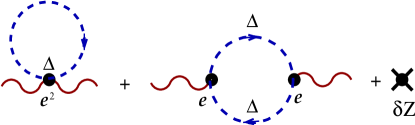
Figure 1: The one-loop diagrams contributing to the photon self-energy.

After some algebra, the one-loop self-energy $[^{\mu}\Pi^{\nu}]$ can be recast in the form

$$i[^{\mu}\Pi^{\nu}](x,x^{\prime}) = \eta^{\mu\rho}\eta^{\nu\sigma}\Big{(}\eta_{\rho\sigma}\partial^{\prime}\cdot\partial-\partial^{\prime}_{\rho}\partial_{\sigma}\Big{)}i\Pi^{(1)}(x,x^{\prime})$$ (5)

$$+ \!\!\eta^{\mu i}\eta^{\nu j}\Big{(}\eta_{ij}\partial_{l}^{\prime}\partial_{l}-\partial_{i}^{\prime}\partial_{j}\Big{)}i\Pi^{(2)}(x,x^{\prime}),\!\!$$

where

$$\!\!\!i\Pi^{(1)}(x,x^{\prime})\!\!\! = \!\!\!\frac{e^{2}}{8\pi^{4}}\!\left[\frac{1}{6\Delta x^{4}}\!-\!\frac{1}{\eta\eta^{\prime}}\left(\!\frac{1}{\Delta x^{2}}\!+\!\frac{\ln(H^{2}\Delta x^{2})}{2\Delta x^{2}}\!\right)\right]$$ (6)

$$i\Pi^{(2)}(x,x^{\prime})\!\!\! = \!\!\!\frac{e^{2}}{8\pi^{4}}\frac{1}{\eta^{2}{\eta^{\prime}}^{2}}\!\left[\frac{1}{2}\ln(H^{2}\Delta x^{2})\!+\!\frac{1}{8}\ln^{2}(H^{2}\Delta x^{2})\right].$$

The first term in (6) is the standard Minkowski vacuum contribution. This term is singular in the (ultraviolet) coincident limit $x\rightarrow x^{\prime}$, while the other terms originate from the nonconformal coupling of scalar fields to gravity in the de Sitter background and are completely integrable. The ultraviolet problems are resolved by using dimensional regularization, that is by calculating in $D$ spacetime dimensions and, subsequently, by renormalizing the self-energy. The result of this rather technical analysis, which we present in ProkopecTornkvistWoodard:2002 , is that $i\Pi^{(1)}\to i\Pi^{(1)}_{\rm ren}$ , where

$$\!\!\!\!i\Pi^{(1)}_{\rm ren}(x,x^{\prime})=i\,\delta\Pi_{\rm anom}(x,x^{\prime})+\frac{e^{2}}{8\pi^{4}}\bigg{[}\partial^{\prime}\cdot\partial\,\frac{\ln(\mu^{2}\Delta x^{2})}{24\Delta x^{2}}$$

$$+\;\frac{1}{\eta\eta^{\prime}}\partial^{\prime}\cdot\partial\left(\frac{1}{16}\ln^{2}(H^{2}\Delta x^{2})+\frac{1}{8}\ln(H^{2}\Delta x^{2})\right)\bigg{]},\quad$$ (8)

and $i\Pi^{(2)}_{\rm ren}=i\Pi^{(2)}$ remains unchanged. Here, $\mu$ is the renormalization scale and

$$i\,\delta\Pi_{\rm anom}(x,x^{\prime})=-i\,\frac{\alpha_{e}}{6\pi}\,\ln(a)\,\delta^{4}(x-x^{\prime})$$ (9)

[with $\alpha_{e}=e^{2}/4\pi$] is a local, anomalous contribution resulting from an imperfect cancellation in expanding backgrounds between the local term and counterterm in Fig. 1.

Upon combining the classical action $S_{0}$ with the anomaly contribution $\delta S_{\rm anom}$, we get

$$\!\!\!\!\!\!\!\!S_{0}+\delta S_{\rm anom}=-\frac{1}{2}\int d^{4}xd^{4}x^{\prime}A_{\mu}(x)\bigg{\{}(\eta^{\mu\nu}\partial^{\prime}\cdot\,\partial-{\partial^{\mu}}^{\prime}\partial^{\nu})$$

$$\quad\quad\times\bigg{[}\bigg{(}1+\frac{\alpha_{e}}{6\pi}\ln\Big{(}\frac{a}{a_{0}}\Big{)}\bigg{)}\delta^{4}(x-x^{\prime})\bigg{]}\bigg{\}}A_{\nu}(x^{\prime}).$$ (10)

This is the scalar electrodynamics equivalent of the Dolgov anomaly Dolgov:1981 ; MazzitelliSpedalieri:1995 . Since the anomalous contribution to the effective action is proportional to $\ln a$, we infer that the anomaly affects the photon dynamics quite mildly Prokopec:2001 ; MazzitelliSpedalieri:1995 when compared with the effect of the photon mass, which contributes as $\propto a^{2}$ and hence is parametrically much larger.

The transverse structure of the vacuum polarization (5) implies that the Ward identities $\partial_{\mu}[^{\mu}\Pi^{\nu}]=0=\partial^{\prime}_{\nu}[^{\mu}\Pi^{\nu}]$ are obeyed, so that gauge invariance remains unbroken. The structure of our result (5)-(8) is very similar to that of thermal QED LeBellac:1996 , which may have something to do with regarding inflationary particle production as Hawking radiation. The spacetime generalization of the standard thermal transverse and ‘longitudinal’ projectors are

$$\!\!P_{\rm T}^{\mu\nu}\!\!=\!\eta^{\mu i}\eta^{\nu i}\!\left(\delta_{ij}\!-\!\frac{\partial_{i}^{\prime}\partial_{j}}{\partial_{l}^{\prime}\partial_{l}}\right),\quad\!P_{\rm L}^{\mu\nu}\!\!\!=\!\eta^{\mu\nu}\!\!\!-\!\frac{{\partial^{\mu}}^{\prime}\partial^{\nu}}{\partial^{\prime}\!\cdot\partial}\!-\!P_{\rm T}^{\mu\nu}\!\!,\,$$ (11)

while the transverse and ‘longitudinal’ polarizations are

$$\Pi_{t}(x,x^{\prime}) = \partial^{\prime}\cdot\partial\,\Pi^{(1)}_{\rm ren}(x,x^{\prime})+\nabla^{\prime}\cdot\nabla\,\Pi^{(2)}_{\rm ren}(x,x^{\prime})\,,$$

$$\Pi_{l}(x,x^{\prime}) = \partial^{\prime}\cdot\partial\,\Pi^{(1)}_{\rm ren}(x,x^{\prime}).$$ (12)

However, this analogy has its limitations. The absence of time-translation invariance in our case makes it non-trivial to extract local physical quantities such as the photon mass or dissipative rate. This is nevertheless possible. Below, we perform a perturbative analysis and show how one can extract a local photon mass from the self-energy (5)-(8).

4. Photon mass. In order to study the effects of the photon self-energy (5)-(8) on the photon propagation, we make use of the Schwinger-Keldysh formalism SchwingerKeldysh:1961-64 ; DeWittJordan:1967-86 and write the photon field equation of motion as follows:

$$\partial_{\nu}F^{\nu\mu}+\int d^{4}x^{\prime}[^{\mu}\Pi_{\rm ren}^{{\rm r}\nu}](x,x^{\prime})A_{\nu}(x^{\prime})=0,$$ (13)

where $[^{\mu}\Pi_{\rm ren}^{{\rm r}\nu}](x,x^{\prime})\equiv[^{\mu}\Pi^{\nu}_{++}](x,x^{\prime})+[^{\mu}\Pi^{\nu}_{+-}](x,x^{\prime})$ defines the retarded photon self-energy in terms of the Feynman $[^{\mu}\Pi^{\nu}_{++}]$ and Wightman $[^{\mu}\Pi^{\nu}_{+-}]$ self-energies so that the photon propagation is manifestly causal. The tensors $[^{\mu}\Pi^{\nu}_{++}]$ and $[^{\mu}\Pi^{\nu}_{+-}]$ are obtained from (5)-(8) by making the replacements $\Delta x^{2}\rightarrow\Delta x^{2}_{++}=-(|\eta-\eta^{\prime}|-i\epsilon)^{2}+\mbox{$|\vec{x}-\vec{x}^{\prime}|^{2}$}$ and $\Delta x^{2}\rightarrow\Delta x^{2}_{+-}=-(\eta-\eta^{\prime}+i\epsilon)^{2}+|\vec{x}-\vec{x}^{\prime}|^{2}$, respectively ProkopecTornkvistWoodard:2002 ; DeWittJordan:1967-86 .

Since the vacuum polarization is only known to one loop order we solve Eq. (13) perturbatively, expanding the photon wave function as

$$A_{\mu}=A_{\mu}^{(0)}+A_{\mu}^{(1)}+\ldots.$$ (14)

Here $A_{\mu}^{(1)}={\cal O}(e^{2})$ is the one-loop amplitude, $A_{\mu}^{(0)}=\varepsilon_{\mu}\,e^{ik\cdot x}$ (with $k_{0}=\pm|\vec{k}|$) is the plane-wave solution to the free Maxwell equation, and $\varepsilon_{\mu}$ is the (transverse) photon polarization vector, which in Lorentz gauge satisfies $\varepsilon_{0}=0$, $\vec{\varepsilon}\cdot\vec{k}=0.$ The one-loop contribution to Eq. (13) then reads

$$\Big{(}\eta^{\mu\nu}\partial^{2}-\partial^{\mu}\partial^{\nu}\!\Big{)}A^{(1)}_{\nu}(x)+\!\int\!\!d^{\,4}\!x^{\prime}\,[^{\mu}\Pi_{\rm ren}^{{\rm r}\nu}](x,x^{\prime})A^{(0)}_{\nu}(x^{\prime})=0.$$ (15)

We are primarily interested in photons that are subhorizon ($k\gg H$) at the initial time $\eta_{0}=-H^{-1}$, and then become superhorizon at some later time $\eta$, $k_{\rm phys}=k/a(\eta)\ll H$, as illustrated in Fig. 2. Upon inserting equations (5), (LABEL:ph-m.11) and (8) into (15), we obtain the following approximate equation for the gauge field ProkopecTornkvistWoodard:2002

$$\Big{(}\eta^{\mu\nu}\partial^{2}-\partial^{\mu}\partial^{\nu}\Big{)}A^{(1)}_{\nu}-a^{2}m_{\gamma}^{2}\,\eta^{\mu\nu}\!A^{(0)}_{\nu}=0,$$ (16)

When evaluated at the leading logarithmic order in $k/H$ and $Ha/k$, the photon mass-squared is

$$m_{\gamma}^{2}=\frac{e^{2}H^{2}}{2\pi^{2}}\ln\frac{k}{H}.$$ (17)

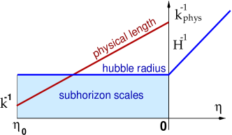
Figure 2: Evolution of the physical scales in de Sitter inflation.

In what follows we shall discuss the origin and the physical relevance of this result. Note first that we have calculated only the leading logarithmic contribution to the photon mass. This will be a good approximation for modes which satisfy $\ln({k}/{H})\gg 1$. The mass (17) corresponds to that of space-like transverse excitations, so it is associated with the transverse polarization $\Pi_{t}$ in (12).

Even though the scalar excitations produced by an inflationary universe are not thermal, one commonly defines the ’Hawking temperature’ $T_{H}=H/2\pi$. In terms of this temperature the photon mass-squared (17) is $m_{\gamma}^{2}=2{e^{2}}T_{H}^{2}\ln(k/H)$. The logarithmic enhancement is a consequence of the nonthermal nature of the spectrum of charged scalar excitations.

The mathematics of our photon mass generation mechanism bears an interesting resemblance to that of the Schwinger model Schwinger:1962 in which the photon acquires a mass $m_{\gamma}^{2}=e^{2}/\pi$. In flat, two dimensional, scalar QED the charged field propagators are logarithmic, which results in the vacuum polarization failing to vanish on shell. The scalar propagator goes like $1/{\Delta x}^{2}$ in 3+1 dimensional flat space, and the photon stays massless. In de Sitter background the scalar propagator has a logarithmic tail which is responsible for our mass generation effect. The two extra spatial dimensions are compensated, in the integration, by two factors of $1/\eta^{\prime}$, and the net result is quite similar to Schwinger’s.

We now relate the photon mass (17) to the Hartree-approximation result $(m_{\gamma}^{2})_{\rm Hartree}=2e^{2}\langle\Omega|\phi^{\dagger}\phi|\Omega\rangle$ considered in DavisDimopoulosProkopecTornkvist:2000 . The Hartree mass arises from the local contribution to the vacuum polarization (4), represented by the first diagram in Fig. 1, and can be estimated by taking the coincident limit of the propagator (3),

$$\langle\Omega|\phi^{\dagger}(x)\phi(x)|\Omega\rangle_{\rm finite}\approx({H^{2}}/{4\pi^{2}})\,\ln a~{},$$ (18)

where we subtracted the initial (vacuum) contribution at $\eta=\eta_{0}$ [with $a(\eta_{0})=1$]. The Hartree mass exactly agrees with our result (17) if one makes the reasonable assumption that a mode with comoving wave number $k$ freezes in at $a(\eta)=k/H$, when the mode’s physical wavelength redshifts beyond the causal horizon.

On the other hand, it is premature to claim more than that the field equation (16) is consistent with the presence of a photon mass. The actual vacuum polarization is nonlocal and, moreover, our perturbative result (17) for the mass arises from a genuinely nonlocal contribution ProkopecTornkvistWoodard:2002 , since the local term that gives the Hartree mass is exactly canceled by a term from the nonlocal diagram in Fig. 1. To prove that superhorizon modes approach the behavior of a massive photon would require gaining control over higher loop corrections and then solving the integral-differential equation (13). We expect that higher loops induce corrections at most of the order of $\alpha_{e}\ln(k/H)$ relative to the one-loop perturbative result (17). If this conjecture is confirmed, the one-loop equation (13) would suffice to study the photon field dynamics in inflation, provided that $\alpha_{e}\ln(k/H)\ll 1$ is satisfied. A detailed investigation of this question will be the subject of future work.

In order to investigate potentially observable effects of a dynamically generated photon mass in inflation, it would be necessary to solve the dynamical equation for the photon in inflation and match it onto solutions for the radiation and matter eras. The result may be the generation of cosmological magnetic fields that seed the galactic dynamo mechanism DavisDimopoulosProkopecTornkvist:2000 . However, in order to perform a reliable analysis of photon propagation in inflation, a more detailed analysis of the photon field equation (13) is required. We postpone this analysis for a later publication.

5. Acknowledgements. We wish to thank Anne Davis and Konstantinos Dimopoulos for work on related issues, and Misha Shaposhnikov for pointing out possible limitations of the Hartree approximation. This work was partially supported by DOE contract DE-FG02-97ER41029 and by the IFT of the University of Florida.

References

- (1) L. de Broglie, La Méchanique Ondulatoire du Photon, Une Nouvelle Théorie de la Lumière, pp. 39-40, Vol. 1, (Hermann, Paris, 1940). E. Schrödinger, Proc. Roy. Irish Acad. A49 (1943) 133. L. Bass and E. Schrödinger, Proc. Roy. Soc. (London) A232 (1955) 1.
- (2) E. R. Williams, J. E. Faller and H. A. Hill, Phys. Rev. Lett. 26 (1971) 721.
- (3) E. Fischbach, H. Kloor, R. A. Langel, A. T. Liu and M. Peredo, Phys. Rev. Lett. 73 (1994) 514.
- (4) L. J. Davis, A. S. Goldhaber and M. M. Nieto, Phys. Rev. Lett. 35 (1975) 1402.
- (5) A. S. Goldhaber and M. M. Nieto, Rev. Mod. Phys. 43 (1971) 277.
- (6) I. T. Drummond and S. J. Hathrell, Phys. Rev. D 22 (1980) 343.
- (7) A. D. Dolgov, Sov. Phys. JETP 54 (1981) 223 [Zh. Eksp. Teor. Fiz. 81 (1981) 417].
- (8) T. Prokopec, astro-ph/0106247.
- (9) M. S. Turner and L. M. Widrow, Phys. Rev. D 37 (1988) 2743.
- (10) A. D. Dolgov, Phys. Rev. D 48 (1993) 2499 [hep-ph/9301280].
- (11) J. S. Schwinger, Phys. Rev. 128 (1962) 2425.
- (12) K. Dimopoulos, T. Prokopec, O. Törnkvist and A. C. Davis, Phys. Rev. D [astro-ph/0108093].
- (13) A. C. Davis, K. Dimopoulos, T. Prokopec and O. Törnkvist, Phys. Lett. B 501 (2001) 165 [astro-ph/0007214].
- (14) P. P. Kronberg, Rept. Prog. Phys. 57 (1994) 325.
- (15) O. Törnkvist, A. C. Davis, K. Dimopoulos and T. Prokopec, astro-ph/0011278.
- (16) E. N. Parker, Cosmic magnetic fields (Clarendon, Oxford, England, 1979).
- (17) A.-C. Davis, M. Lilley and O. Törnkvist, Phys. Rev. D 60 (1999) 021301 [astro-ph/9904022].
- (18) D. Grasso and H. R. Rubinstein, Phys. Rept. 348 (2001) 163 [astro-ph/0009061].
- (19) T. Prokopec, O. Törnkvist and R. Woodard, in preparation.
- (20) L. H. Ford and L. Parker, Phys. Rev. D 16 (1977) 245. A. Vilenkin and L. H. Ford, Phys. Rev. D 26 (1982) 1231. B. Allen and A. Folacci, Phys. Rev. D 35 (1987) 3771. N. C. Tsamis and R. P. Woodard, Class. Quant. Grav. 11 (1994) 2969.
- (21) F. D. Mazzitelli and F. M. Spedalieri, Phys. Rev. D 52 (1995) 6694 [astro-ph/9505140].
- (22) Michel Le Bellac, Thermal field theory (Cambridge University Press, 1996) [ISBN 0 521 46040 9].
-
(23)
J. Schwinger,
J. Math. Phys. 2 (1961) 407.
L. V. Keldysh, Zh. Eksp. Teor. Fiz. 47 (1964) 1515 [Sov. Phys. JETP 20 (1964) 1018]. -
(24)
B. S. DeWitt,
Phys. Rev. 162 (1967) 1195.
R. D. Jordan, Phys. Rev. D 33 (1986) 444.