Radiation pressure instability driven variability in the accreting black holes

Abstract

The time dependent evolution of the accretion disk around black hole is computed. The classical description of the $\alpha$-viscosity is adopted so the evolution is driven by the instability operating in the innermost radiation-pressure dominated part of the accretion disk. We assume that the optically thick disk always extends down to the marginally stable orbit so it is never evacuated completely. We include the effect of the advection, coronal dissipation and vertical outflow. We show that the presence of the corona and/or the outflow reduce the amplitude of the outburst. If only about half of the energy is dissipated in the disk (with the other half dissipated in the corona and carried away by the outflow) the outburst amplitude and duration are consistent with observations of the microquasar GRS 1915+105. Viscous evolution explains in a natural way the lack of direct transitions from the state C to the state B in color-color diagram of this source. Further reduction of the fraction of energy dissipated in the optically thick disk switches off the outbursts which may explain why they are not seen in all high accretion rate sources being in the Very High State.

1 Introduction

Accreting black holes are strongly variable sources in all ranges of timescales. Short time-scale variability is usually described through the Fourier analysis and the state of the source can be identified by a characteristic shape of the power spectra of galactic black holes (GBH). Physical interpretation of this variability is not known although some hypotheses were formulated. Since the power spectra of X-ray emission for sources in the Low (hard) and High (soft) state are clearly different the underlying mechanism may also be different in both cases. Furthermore, the Very High State is also characterized by distinctively different variability and spectral properties so yet another mechanism may be responsible for variations in that spectral state. The nature of this particular variability is the subject of our paper.

Belloni et al. (2000) performed a detailed observational analysis of the variability patterns in the microquasar GRS 1915+105. It was previously found (Belloni et al. 1997a, 1997b), that during the high luminosity states the spectrum of this source is dominated by a thermal, disk-like component and the variability was modeled phenomenologically by periodic disappearance of the inner accretion disk (Feroci et al. 1999). Nayakshin, Rappaport & Melia (2000) and Janiuk, Czerny & Siemiginowska (2000) suggested recently, that the variability of the microquasar GRS 1915+105 in its Very High State displays features characteristic for the limit cycle behaviour well known in CV but with the timescales orders of magnitude shorter.

The limit cycle behaviour of CV is caused by the disk thermal and viscous instability in the region of partial ionization of the hydrogen (Smak 1984, Meyer & Meyer-Hofmeister 1984) and was studied in the context of time evolution of these objects (Cannizzo 1993, Hameury et al. 1998). The same instability is also responsible for the eruptions of many X-ray transients, including GBH, and its characteristic timescales are days/years (Cannizzo et al. 1995). As the accretion disks around supermassive black holes are expected to have similar properties, also for these objects the analysis of the thermal and viscous instability was performed (Lin & Shields 1986, Mineshige & Shields 1990). The evolution of the accretion disk in AGN driven by the partial ionization of the hydrogen was computed e.g. in Siemiginowska et al. (1996).

However, the standard model of accretion disk by Shakura & Sunyaev (1973) predicts also the existence of additional instability due to the radiation pressure, with timescales orders of magnitude shorter, which is therefore a good candidate to explain the behaviour of the microquasar, as well as the short term variability in AGNs. This radiation pressure instability was first noticed in Pringle, Rees &Pacholczyk (1973) and studied in Lightman & Eardley (1974) and Shakura & Sunyaev (1976).

In order to obtain a limit cycle behaviour in the range of radiation pressure instability, some stabilizing mechanism must be taken into account. Abramowicz et al. (1988) found that radial advection has stabilizing effect on the disk at high accretion rates. This was adopted by Honma et al. (1991) in the disk evolution computations. Thermal stability of the transonic accretion disks was studied in Szuszkiewicz & Miller (1997) and the limit cycle behaviour was confirmed by calculations of Szuszkiewicz & Miller (1998).

Detailed analysis of the stability properties of the disk models in comparison with the observational data leads to the conclusion that in order to obtain better qualitative agreement with the observations, certain modifications of the theoretical models are necessary. Szuszkiewicz (1990) studied slim disk models with viscosity prescriptions different from standard $\alpha$ viscosity of Shakura & Sunyaev (1973) in order to obtain appropriate outburst amplitudes. Also other modified viscosity laws were introduced (e.g. Milsom et al. 1994, Taam et al. 1997). Moreover, several authors postulated that $\sim 90\%$ of the energy generated in the disk is radiated away by the disk corona (Nayakshin et al. 2000) or that energy carried by jet has to be included in the model (Janiuk, Czerny & Siemiginowska 2000). However, while the last modification seems to be well supported by the observational data, the dominating role of the hot corona is clearly in contradiction with the observed spectral shape of the sources in the Very High State.

In the present paper we propose the time dependent model of an accretion disk and we calculate the disk evolution based on radiation pressure instability. We study in detail the model properties and its sensitivity to the adopted parameters. We consider the role of advection in the energy budget and we take into account the possible effects of an outflow and a corona, which are consistent with our current understanding of the accretion flow at high luminosity to the Eddington luminosity ratio. Finally, we compare the resulting lightcurves and spectra with the observations.

2 Radiation pressure instability

In this section we analyze the local instability of an accretion disk caused by the radiation pressure domination. The simplest approach to the study of the disk stability is based on the vertically averaged description of the disk structure (Shakura & Sunyaev 1973, Shakura & Sunyaev 1976). The vertically averaged model offers an easy qualitative insight into the disk properties. However, this approach is neither accurate nor unique. Various approaches to the averaging were used in the literature and they differ in detailed predictions of the disk stability.

Paczyński & Bisnovatyi-Kogan (1981) introduced the politropic approximation to the disk vertical structure which resulted in the presence of additional numerical factors, ranging from 0.5 to 6.0, in the averaged equations. The same values were later adopted by Abramowicz et al. (1988). Honma et al. (1991) adopted different coefficients ranging from 1.0 to 16.0 and in Nayakshin, Rappaport & Melia (2000) the coefficients were in the range from 0.5 to 2.0. The stability of the disk with advection was also studied within the frame of the vertically averaged quantities (Abramowicz et al. 1988, Szuszkiewicz 1990, Szuszkiewicz, Malkan & Abramowicz 1996). Here we stress that the values of the accretion rate corresponding to the transition from the stable branches to the intermediate unstable branch may well be affected by this approach.

Recent simulations of the local structure of radiation pressure dominated disks performed by Agol et al. (2001), Turner & Stone (2001) and Turner, Stone & Sano (2002) agreed with the analytical models. They confirmed that the radiation pressure dominated disks are unstable, although details of the viscous heating and convection may affect the accretion rate at which the instability occurs. Interestingly, these first simulations also show that the result of the instability could lead in some cases to the disk collapsing to a new gas pressure dominated equilibrium. The long term global evolution effects of the radiation pressure dominated disks have not been calculated so far in the 2D simulations.

Since the full 2D approach to the study of global long timescale disk evolution is very complex, we adopt the 1D+1D approach. Therefore in subsection 2.1 we study the full vertical structure of the accretion disk with standard prescription for the viscosity and advection. Due to this approach in subsection 2.2 we are able to determine uniquely the appropriate numerical coefficients, which are subsequently used in the vertically averaged disk model. In subsection 2.3 we include in the model the presence of a hot corona above the disk and a possibility of a vertical outflow powered by accretion. In subsection 2.4 we describe the shape of the stability curve resulting from the averaged equations and we discuss the role of this stability curve and of the model parameters in the time evolution of the accretion disk.

2.1 Vertical structure of a stationary accretion disk

The disk model at a given radius $r$ is parameterized by the mass of the black hole $M$, accretion rate $\dot{M}$, and the viscosity parameter $\alpha$. In this work we use a standard viscosity prescription, based on the assumption that the viscous stress tensor is proportional to the total pressure $P$:

$$\tau_{\rm r\varphi}=-\alpha P.$$ (1)

While presenting the results, we frequently use the dimensionless accretion rate $\dot{m}$, given by

$$\dot{m}\equiv{\dot{M}\over\dot{M}_{\rm Edd}},$$ (2)

where $\dot{M}_{\rm Edd}$ is the critical (Eddington) accretion rate:

$$\dot{M}_{\rm Edd}={L_{\rm Edd}\over c^{2}\eta}={4\pi GMm_{H}\over\sigma_{T}c\eta}.$$ (3)

The efficiency of accretion is $\eta=1/16$, as it results from the pseudo-Newtonian approximation to the disk accretion (Paczyński & Wiita 1980).

The total energy flux $F_{\rm tot}$ dissipated within the disk at a radius $r$ is determined by the global parameters:

$$F_{\rm tot}={3GM\dot{M}\over 8\pi r^{3}}f(r),$$ (4)

where $f(r)$ represents the boundary condition at the marginally stable orbit:

$$f(r)=1-({r_{\rm ms}\over r})^{3/2}{r-r_{\rm g}\over r_{\rm ms}-r_{\rm g}}$$ (5)

in the pseudo-Newtonian approximation.

The disk vertical structure is described by a set of basic equations: the equation of viscous energy dissipation,

$${dF\over dz}=\alpha P(-{d\Omega_{K}\over dr}),$$ (6)

the hydrostatic equilibrium,

$${1\over\rho}{dP\over dz}=-\Omega_{K}^{2}z,$$ (7)

where the total pressure is the sum of the gas and radiation pressure:

$$P=P_{\rm gas}+P_{\rm rad},$$ (8)

and equation of energy transfer,

$${dT\over dz}=-{3\kappa\rho\over 4acT^{3}}F_{\rm l}.$$ (9)

The latter takes into account the presence of convection which carries non-negligible fraction of energy (see e.g. Shakura, Sunyaev & Zilitinkevich 1978, Dörer et al. 1996):

$$~{}~{}~{}~{}~{}~{}~{}F_{\rm l}=F_{\rm rad}~{}~{}~{}~{}~{}\nabla_{\rm rad}\leq\nabla_{\rm ad}{}$$ (10)

$${}F_{\rm l}=F_{\rm rad}+F_{\rm conv}~{}~{}~{}~{}~{}\nabla_{\rm rad}>\nabla_{\rm ad}{}$$

Here $F_{l}$ is the energy flux transported locally in the direction perpendicular to the equatorial plane, carried either by radiation or by convection. It differs from the flux $F$ due to the presence of radial advection. We introduce the advection term into our set of equations assuming that the fraction of energy radially advected does not depend on the distance from the equatorial plane. Such an approach seems to be justified, since the dependence of the radial velocity on the distance from the equatorial plane is uncertain and it does not influence other equations. Therefore we calculate the required entropy gradients at the equatorial plane, denoting the appropriate thermodynamical quantities with an index $e$. The local energy flux is then given by

$$F_{l}=F_{\rm tot}(1-f_{\rm adv})$$ (11)

and the advected fraction $f_{\rm adv}$ is determined from the global ratio of the total advected flux to the total viscously generated flux (e.g. Paczyński & Bisnovatyi-Kogan 1981, Muchotrzeb & Paczyński 1982, Abramowicz et al. 1988):

$$f_{\rm adv}={F_{\rm adv}\over F_{\rm tot}}=-{2rP_{e}q_{\rm adv}\over 3\rho_{e}GMf(r)},$$ (12)

where

$$q_{\rm adv}=(12-10.5\beta_{e}){dlnT_{e}\over dlnr}-(4-3\beta_{e}){dln\rho_{e}\over dlnr}.$$ (13)

Here $\beta$ is the gas pressure to the total pressure ratio

$$\beta={P_{\rm gas}\over P}.$$ (14)

Defining the advection term through the quantities at the disk equatorial plane is an oversimplification which reflects the fact that the approach to the vertical structure of the disk outlined above does not include any information about the vertical distribution of the radial velocity. The actual flow pattern can be studied only if we allow for the departure from the strict vertical hydrostatic equilibrium. The computed flow pattern in Keplerian disks is rather complex since the meridional circulation is superimposed on the mean accretion flow (e.g. Siemiginowska 1988). Therefore, there is some uncertainty involved at this stage even in the case of disk vertical structure included.

The frequency-averaged opacity $\kappa$ (Rosseland mean) used in vertical structure computations includes the electron scattering as well as the required free-free and bound-free transitions. The tables are from Alexander, Johnson & Rypma (1983) for log $T<3.8$, from Seaton et al. (1994) for log $T>4.0$ and the value of opacity is interpolated between these two tables for intermediate values of the temperature, as in Różańska et al. (1999). The numerical code which computes the disk vertical structure was developed from the version from Pojmański (1986) and subsequently modified by Różańska et al. (1999).

If the value of the $f_{\rm adv}$ is specified somehow in advance the integration of the disk vertical structure proceeds in a usual way. The boundary conditions to the set of differential equations are specified in the equatorial plane $z=0$ and at the disk surface located at a priori unknown height $z=H$:

$$F(0)=0,~{}~{}F(H)=F_{\rm tot},$$

$$\sigma T^{4}(H)=0.5F_{\rm tot}(1-f_{\rm adv}).$$ (15)

The presence of radial derivatives means that the problem in general should be solved as a global one, after defining the appropriate outer and inner radial boundary conditions. However, here for simplicity we adopt the local approach to advection developed and successfully used by Chen (1995). The numerical value of $q_{\rm adv}$, given by Equation 13, may be specified at each radius by iterations at the two neighbouring radii. This advection term does not depend much on the accretion rate and may well be assumed constant on the thermal equilibrium curve for a given radius. Such a method is correct for disks which are Keplerian and not too close to the marginally stable orbit, where the conditions close to the sonic point are essential (see also Yuan 1999).

2.2 Vertically averaged stationary disk model

In the vertically averaged disk structure the differential equations (6) - (9) may be replaced by the quantities defined as mean values or values determined at the equatorial plane. The numerical coefficients $C_{\rm i}$ are uniquely determined here from the vertical structure model:

$$C_{\rm 1}={\int_{0}^{H}Pdz\over P_{\rm e}H}$$ (16)

$${1\over C_{\rm 2}}={\int_{0}^{H}\rho Fdz\over\rho_{\rm e}F_{\rm rad}H}$$ (17)

$$C_{3}={\int_{0}^{H}\rho zdz\over\rho_{\rm e}H^{2}}$$ (18)

Therefore we can use the vertically averaged relations:

$$F_{\rm tot}=C_{1}{3\over 2}\alpha P\Omega_{K}H$$ (19)

is the local energy flux generated through the $\alpha$ viscosity,

$$F_{\rm l}H=C_{2}{acT^{4}\over 3\kappa\rho}$$ (20)

is the local emitted flux, and the hydrostatic equilibrium is expressed as:

$${P\over\rho}=C_{3}\Omega_{K}^{2}H^{2}.$$ (21)

From the disk vertical structure calculations we obtained numerical coefficients $C_{1}$, $C_{2}$ and $C_{3}$ approximately equal to 0.4, 2.0 and 0.17 (they only weakly depend on the accretion rate and viscosity). Using these coefficients we can write for any given radius the vertically averaged, time-independent, energy balance equation:

$$C_{1}H{3\over 2}\alpha P\Omega_{K}=C_{2}{1\over H}{acT^{4}\over 3\kappa\rho}-{1\over 2\pi r}\dot{M}T{dS\over dr},$$ (22)

where the left hand side refers to the viscous energy dissipation and the right hand side describes energy losses due to diffusion of radiation and advection. The entropy gradient is equal to:

$$T{dS\over dr}r={P\over\rho}q_{\rm adv}$$ (23)

where $q_{\rm adv}$ is described by the Equation (13) and is approximately constant. The energy balance Equation (22) together with the averaged hydrostatic equilibrium Equation (21) allow us to compute the stability curve on the surface density versus temperature ($\Sigma-T$) plane. These stationary solutions are presented in Section 2.4.

2.3 Stationary disk with a corona and vertical outflow

Detection of the power law tail in the hard X-ray spectra of black hole X-ray binaries and AGNs (Mushotzky, Done & Pounds 1993, Tanaka & Lewin 1995) indicates, that somewhat hotter medium is present in the vicinity of a standard accretion disk. Here we assume, that this hot gas forms a corona above the disk, which extends down to the marginally stable orbit and dissipates a constant fraction $f_{\rm cor}$ of the total accretion energy. This energy does not contribute to the disk black body emission, but is stored in the corona and radiated in the hard X-rays.

For a number of objects the presence of a collimated vertical outflow is confirmed (e.g. Mirabel & Rodriguez 1994 for GRS 1915+105). We also include in our model such a possibility, however we do not adopt any collimation mechanism. The plasma ejection is powered by the energy released in the innermost disk parts. Therefore we assume that another fraction of a total energy is converted into the wind and is not seen in the disk multicolor black body emission. We parameterize this fraction using the luminosity to the Eddington luminosity ratio, so that for accretion near the Eddington limit we should expect the outflow to be the strongest. Unlike in the ADAF models, where a powerful wind may take away a considerable amount of mass and angular momentum (Blandford & Begelman 1999), we assume, that in our disk the carried mass and angular momentum may be negligible (see Discussion). Therefore the presence of a wind is reflected only in the energy equation.

The energy balance Equation (22) is modified by the outflow and the corona. In principle, in the time independent model, we could put the outflowing and coronal fractions either in the cooling or in the heating term with no change in the final energy balance. However, in the physical case both the outflow and the corona play their role in cooling of the accretion flow, so in general the emitted flux will have the form:

$$F^{-}=C_{\rm 2}{1\over H}{acT^{4}\over 3\kappa\rho}[(1-f_{\rm cor})(1-f_{\rm out})]^{-1},$$ (24)

where

$$f_{\rm out}=1-{1\over 1+A\dot{m}^{2}}$$ (25)

we take after Nayakshin et al. (2000). Our model parameters are $A$ and $f_{\rm cor}$, which we assume to be constants, ranging from 0 to 1. Below we describe the role of these parameters in the resulting stationary disk solutions.

2.4 The local stability curve

When the energy balance given by Equation 22 is satisfied, the stationary local disk solutions form a characteristic S curve on the $\Sigma-T$ plane (alternatively on the vertical axis we may plot accretion rate $\dot{M}$ instead of the temperature). In this section we consider the curves calculated for the $10M_{\rm\odot}$ black hole. In the case of a supermassive black hole the disk temperature is $\sim 2$ orders of magnitude lower and the surface densities may reach $\sim 10$ times higher values for a given $R/R_{Schw}$. It results in shifting the entire stability curve down and right on the $\Sigma-T$ diagram.

The accretion disk is thermally and viscously unstable when ${\partial\dot{M}\over\partial\Sigma}<0$ (Lightman & Eardley 1974, Meyer & Meyer-Hofmeister 1981). This is the case for the accretion rates in the range $(\dot{m}_{1},\dot{m}_{2})$, where the S curve has a negative slope. The lower branch of the curve represents stable solutions, resulting from the gas pressure domination. The intermediate unstable branch appears due to radiation pressure domination, while the upper hot branch is stabilized by advection (Abramowicz et al. 1988). The upper and lower transition points $\dot{m}_{1}$ and $\dot{m}_{2}$ depend on the global model parameters (i.e. $M$ and $\alpha$) as well as on the local distance $r$. The dependence on the global parameters is relatively weak, but there is a strong dependence on the radial location $r$: a change of $r$ results mostly in a strong shift of the entire curve up or down on the diagram. It translates into strong dependence of the extension of the radiation-pressure dominated disk region on the accretion rate (e.g. Hure 1998, Janiuk & Czerny 2000).

In Figure 1 we plot the solutions for several disk radii. If the external accretion rate does not exceed a critical value, the whole disk remains in the cold, stable regime and the matter is transported inwards with constant velocity. However, for higher external accretion rates the inner disk parts may find themselves in an unstable mode. Then the disk undergoes oscillations, heating up and cooling down in a cycle. This may cause the observed luminosity outbursts or flickering. The range of accretion rates for which the disk is locally unstable varies across the disk. It is wider at small radii and becomes narrower at larger radii. This effect is even stronger, if the full vertical structure is computed instead of the constant $C_{\rm i}$ coefficients in the vertically averaged model. In this case at large radii, $r>200R_{\rm Schw}$ the whole intermediate branch of the S curve gets a positive slope and the instability vanishes. As a result the outer parts of the disk are stable, while the inner parts may undergo oscillations.

Figure 1: The stability curves calculated for $M=10M_{\odot}$, and 4 different radii : $R=10R_{\rm Schw}$ (solid curve), $R=60R_{\rm Schw}$ (dotted curve), $R=140R_{\rm Schw}$ (short-dashed curve) and $R=290R_{\rm Schw}$ (long-dashed curve). The viscosity parameter $\alpha=10^{-2}$. The effects of outflow and corona are neglected. Note, that on the vertical axis we plot local dimensionless accretion rate, $\dot{m}=\dot{M}/\dot{M}_{Edd}$, instead of the disk temperature.

The critical accretion rate, above which the disk becomes unstable, as well as the outbursts amplitude depend on the location of the turning points $\dot{m}_{1}$ and $\dot{m}_{2}$ on the stability curve. This is determined by the presence and the strength of the disk hot corona and/or outflow.

In Figure 2 we plot the stability curves at location $R=10R_{\rm Schw}$, resulting from different assumptions about the fraction of energy dissipated in the corona. When the corona is neglected, the lower turning point corresponds to a very small accretion rate ($\dot{m}_{1}\sim 0.06$) and the outburst amplitudes should be very large. The presence of the corona increases the critical accretion rate and reduces the size of the unstable branch, which results in a reduction of the outbursts amplitude.

Figure 2: The stability curves calculated for $M=10M_{\odot}$, $R=10R_{\rm Schw}$ and 4 values of the fraction of energy dissipated in the corona: $f_{\rm cor}=0.0$ (solid curve), $f_{\rm cor}=0.3$ (dotted curve), $f_{\rm cor}=0.5$ (short-dashed curve) and $f_{\rm cor}=0.9$ (long-dashed curve). The viscosity parameter $\alpha=10^{-2}$. The outflow effect is neglected.

In Figure 3 we plot the solutions obtained for different strengths of the outflow. The strong outflow suppresses the instability at high temperatures and reduces the amplitude of an outburst. However, it does not affect the cold stable branch and has no influence on the lower turning point on the stability curve.

Figure 3: The stability curves calculated for $M=10M_{\odot}$, $R=10R_{\rm Schw}$ and 4 values of the outflow parameter A (see Equation 25): 0.0 (solid curve), 0.025 (dotted curve), 0.125 (short-dashed curve) and 0.325 (long-dashed curve). The viscosity parameter $\alpha=10^{-2}$. The effect of the corona is neglected.

The evolution time scale and duration of an outburst is determined by the viscosity. Here we use the constant viscosity parameter $\alpha$. In Figure 4 we plot the dependence of the disk solutions on this parameter. The stability curve is shifted almost horizontally with $\alpha$. Therefore the viscosity parameter does not influence outburst amplitudes, while its value may make them last shorter or longer.

Figure 4: The stability curves calculated for $M=10M_{\odot}$, $R=10R_{\rm Schw}$ and 3 values of viscosity parameter: $\alpha=10^{-1}$ (solid curve), $\alpha=10^{-2}$ (dotted curve), and $\alpha=10^{-3}$ (dashed curve). The corona and outflow effects are neglected.

3 Time dependent disk

In this section we describe the time dependent disk model. Here we treat the disk radial structure independently from the vertical one, which is included in our calculations via the coefficients $C_{\rm i}$ in the averaged equations. The crucial parameter, which links the radial and vertical disk structures, is the viscosity parameter $\alpha$. The viscosity mechanism is responsible for both radial transfer of the material inwards and for the local dissipation of energy, which in turn is either radiated vertically or advected. Once $\alpha$ is specified, we adopt the vertically averaged equations in the time evolution of the disk.

3.1 The basic equations

The energy balance expressed by the Equation (22) gives the stationary solution in the $\Sigma-T$ plane. In order to construct the time dependent model we solve the two basic equations for $\Sigma(r,t)$ and $T(r,t)$, following the evolution of the accretion disk. The mass conservation equation:

$${\partial\Sigma\over\partial t}={1\over 2\pi r}{\partial\dot{M}\over\partial r},$$ (26)

where

$$\dot{M}=-2\pi r\Sigma v_{\rm r},$$ (27)

is combined with the angular momentum conservation equation:

$$\dot{M}{d\over dr}\big{(}r^{2}\Omega\big{)}=-{\partial\over\partial r}\big{(}2\pi r^{2}T_{\rm r\varphi}\big{)}.$$ (28)

Here $\Omega$ is the Keplerian velocity and the $r\varphi$ component of the stress tensor is equal to $T_{\rm r\varphi}=\alpha PH=(3/2)\Omega\nu\Sigma$. $P$ is the total pressure, $H$ is the disk height, $\nu$ denotes the kinematic viscosity and $v_{\rm r}$ is the radial velocity. From these equations we obtain the equation of the surface density evolution:

$${\partial\Sigma\over\partial t}={1\over r}{\partial\over\partial r}\Big{(}3r^{1/2}{\partial\over\partial r}\big{(}r^{1/2}\nu\Sigma\big{)}\Big{)}.$$ (29)

The disk temperature evolves due to the departure from the thermal energy conservation:

$$\Sigma T{dS\over dt}=Q^{+}-Q^{-}.$$ (30)

Here we adopt viscous heating

$$Q^{+}=C_{1}(3/2)\Omega\alpha PH$$ (31)

and radiative cooling

$$Q^{-}=C_{2}[(1-f_{\rm cor})(1-f_{\rm out})]^{-1}(4\sigma/3\kappa)(T^{4}/\Sigma).$$ (32)

The coefficients $C_{\rm 1}$ and $C_{\rm 2}$ were defined in Section 2.2. Combining Equation (30) with time-dependent forms of Equations (23) and (13) we obtain the energy equation:

$${\partial\ln T\over\partial t}+v_{\rm r}{\partial\ln T\over\partial r}={}$$

$${}={4-3\beta\over 12-10.5\beta}\Bigg{(}{\partial\ln\Sigma\over\partial t}-{\partial\ln H\over\partial t}+{}$$

$${}+v_{\rm r}{\partial\ln\Sigma\over\partial r}\Bigg{)}+{Q^{+}-Q^{-}\over(12-10.5\beta)PH}{}.$$ (33)

The radial velocity is given by:

$$v_{\rm r}=-{3\over\Sigma}r^{-1/2}{\partial\over\partial r}\big{(}\nu\Sigma r^{1/2}\big{)}.$$ (34)

The corona and the vertical outflow, parameterized by $f_{\rm cor}$ and $f_{\rm out}$ (see Section 2.3), play a crucial role in our calculations. In principle, they could contribute either to the cooling or to the heating of the disk, and therefore influence strongly the results of the time evolution. Here we choose again the physical case, e.g. corona and outflow as the disk cooling mechanisms, consistently with our stationary solution. In the following we assume that they add to the cooling $Q^{-}$, while the heating term $Q^{+}$ includes only viscosity. The corona parameter $f_{\rm cor}$ is assumed constant with time and radius, while $f_{\rm out}$ depends on time and radius of the disk via the local accretion rate $\dot{m}(r,t)$; in this case the constant parameter of the evolution is $A$ (see Equation 25).

3.2 Numerical method

We solve the equations (29) and (33) via explicit method, using the constant time step, comparable to the thermal time scale (Wallinder 1991):

$$t_{\rm therm}=8.75\times 10^{-5}{r^{1/2}\over\alpha}(r-1){M\over M_{\rm\odot}}~{}~{}~{}~{}[s]$$ (35)

where r is the radius expressed in Schwarzschild radii.

The viscous time scale depends on the disk thickness:

$$t_{\rm visc}\sim{\Sigma\over{\partial\Sigma\over\partial t}}\sim{1\over\alpha\Omega}\Big{(}{r\over H}\Big{)}^{2}$$

$$t_{\rm therm}\sim{T\over{\partial T\over\partial t}}\sim{1\over\alpha\Omega}$$

$${t_{\rm therm}\over t_{\rm visc}}\sim\Big{(}{H\over r}\Big{)}^{2}.$$ (36)

For typical values of $H/r$ in our model the viscous time scales are 3 - 4 orders of magnitude longer than the thermal time scales.

The equation (29) is transformed into a simple diffusion equation due to the convenient change of variables (Smak 1984):

$${\partial\Xi\over\partial t}={12\over y^{2}}{\partial^{2}\over\partial y^{2}}\big{(}\Xi\nu\big{)}$$

$$y=2r^{1/2}~{}~{}~{}~{}~{}~{}~{}~{}\Xi=y\Sigma$$ (37)

On the uniform radial grid in $y$ we compute in every time step the new values of the 6 variables: $\Xi_{\rm j}^{n}$, $T_{\rm j}^{n}$, $P_{\rm j}^{n}$, $H_{\rm j}^{n}$, $\beta_{\rm j}^{n}$ and $\nu_{\rm j}^{n}$, where $j$ is the number of radial zone and $n$ is the number of a time step. Initial values are taken from the stationary solution on the lower branch of the $\Sigma-T$ curve. The boundary condition on the inner disk radius, $3R_{\rm Schw}$, is that $T_{\rm in}=\Sigma_{\rm in}=0$. The outer disk radius is chosen to have a stable solution, determined by the external, constant accretion rate $\dot{m}_{\rm ext}$ This assumption implies, that a certain amount of the angular momentum is taken away at the outer radius of the computed disk region. The typical radial extension in our calculations was $300R_{\rm Schw}$ and the number of points in the radial grid was 220.

3.3 Results

In this Section we present the results of the time dependent calculations. The main parameters of the model are mass of the central black hole $M$, external accretion rate $\dot{m}_{\rm ext}$, viscosity $\alpha$, coronal fraction $f_{\rm cor}$ and outflow strength $A$. Throughout this work we assumed the mass of the central object equal to 10 $M_{\odot}$, which is appropriate order of magnitude for galactic black hole binary systems. The viscosity was constant in the disk and in every model we adopted $\alpha=0.01$.

The external accretion rate is the accretion rate outside the region of the radiation pressure instability, at the outer radius, which in most cases was fixed at 300 $R_{\rm Schw}$. This accretion rate value was chosen in the range $\dot{m}_{\rm ext}=0.19-0.71$, so that the inner disk parts were unstable. However, we did not take into account any effects connected with possible ionization or gravitational instability, which may be present further out in the disk. We performed our calculations for the full range of corona and outflow strengths ($f_{\rm cor}$ and $A$ ranging from 0 to 1).

Once all the model parameters are specified, the disk starts to evolve, and tries to reach the state specified by $\dot{m}_{\rm ext}$. At every disk radius the solution is found along the lower branch of the stability curve S, up to the moment when the innermost radii find themselves in the unstable mode. Then the oscillations begin, and the disk temperature and density change periodically with time.

Below we present the results of our calculations. Firstly, we discuss the evolution at the particular disk radius during one cycle, e.g. starting and ending on the lower stable branch of the S curve. This translates into one outburst of the disk total luminosity. Secondly, we show, how the luminosity of the disk changes with time, depending on the assumed corona and outflow efficiencies. Finally, we present the influence of the radiation pressure instability on the geometrical thickness of the accretion disk, and we show an example of the disk spectral energy distribution.

3.3.1 Evolution of the surface density and temperature during one cycle

In Figure 5 we show the evolution of the surface density during one cycle. Between the outbursts the radial dependence of $\Sigma$ is smooth and has a positive slope. The radial inflow through the accretion disk is stable and the material accumulates slowly in the inner region. When the instability starts, the density drops down rapidly in the innermost radii, along with the increasing local accretion rate. The matter is transferred inwards much faster than it is supplied from the outer disk regions and the inner disk empties. At the outer end of the unstable region there appears a local density peak, which shifts outwards as the instability propagates into larger radii. The outburst finishes when there is no more additional matter supply. As the disk cools down, the density in the inner part gradually rises and when the cycle is completed, the flow returns to the initial configuration.

Figure 5: The surface density evolution during a single outburst. Model parameters: $M=10M_{\odot}$, $\alpha=10^{-2}$, $\dot{m}_{\rm ext}=0.7$. The corona share is $f_{\rm cor}=0.5$. The outflow is neglected.

In the outburst the disk temperature rises mostly in the inner disk regions. In Figure 6 we show the temperature evolution during one cycle. The instability begins at the innermost disk radius. It propagates outwards and after several time steps the heat front reaches further regions. The temporal decrease of the temperature in the inner part is characteristic for models with both high external accretion rates and considerable corona share. During this temporal decrease the disk is still heated up in outer regions, and this phase corresponds to the smaller “dip” in the lightcurve. It is followed by the subsequent heating of the entire unstable disk region, which is the cause of the sharp luminosity increase. At the end of the cycle the whole disk cools down rapidly. The cooling front again starts from the inner disk radius and propagates on the thermal time scale. The disk enters into the phase of relative faintness of the inner parts. It may observationally create an impression that the inner disk has been completely evacuated, while actually the disk always extends down to the marginally stable orbit.

Figure 6: The temperature evolution during a single outburst. Model parameters: $M=10M_{\odot}$, $\alpha=10^{-2}$, $\dot{m}_{\rm ext}=0.7$. The corona share is $f_{\rm cor}=0.5$. The outflow is neglected.

The evolution on the $\Sigma-T$ plane depends on the local disk radius. The innermost parts of the disk reach the highest temperatures and if the external accretion rate is high enough, they may even jump to the upper, advection supported branch of the stability curve. This depends on other model parameters, e.g. the strength of the corona and the outflow. Further out the upper branch is never reached and the disk undergoes oscillations in the intermediate unstable region. The outermost parts of the disk always remain on the lower, cold stable branch (see Figure 7).

Figure 7: The evolution on the $\Sigma-T$ plane for four different values of radius: $5.75R_{\rm Schw}$, $9.88R_{\rm Schw}$, $30.5R_{\rm Schw}$ and $140.5R_{\rm Schw}$. The solid line marks the local stability curve and the points represent the solutions of the time dependent disk model. We show the time sequence from the beginning of the evolution through a few outbursts. Model parameters: $M=10M_{\odot}$, $\dot{m}_{\rm ext}=0.65$, $\alpha=0.01$. The corona share is neglected and the outflow efficiency parameter is A = 0.025.

3.3.2 The luminosity of the disk

The total disk luminosity is equal to $L=\int_{R_{\rm in}}^{R_{\rm out}}2\pi rF_{\rm rad}dr$ and it results only from the radiation of the disk. We do not include the fraction radiated by the corona, carried by the outflow or advected. The coronal fraction is assumed constant during the evolution. However, the outflow strength depends on the luminosity to the Eddington luminosity ratio and varies: from negligible value between the outbursts to $f_{\rm out}\sim 0.35$ during the outburst. Therefore, in the absence of an outflow, the resulting outburst amplitude remains constant, being somewhat lower for a disk with a strong corona than for a disk alone. When the outflow is present, the observed outburst amplitude varies during the evolution. The observed luminosity fraction radiated by the accretion disk is equal to $f_{\rm obs}=(1-f_{\rm cor})(1-f_{\rm out})$. Depending on other model parameters, in the case of a strong outflow its luminosity may reach even $f_{\rm out}/f_{\rm obs}=30-70\%$.

Figure 8: The disk lightcurve. Model parameters: $M=10M_{\odot}$, $\dot{m}_{\rm ext}=0.7$, $\alpha=0.01$. The fraction of the energy dissipated in the corona is $f_{\rm cor}=0.5$. The outflow is neglected.

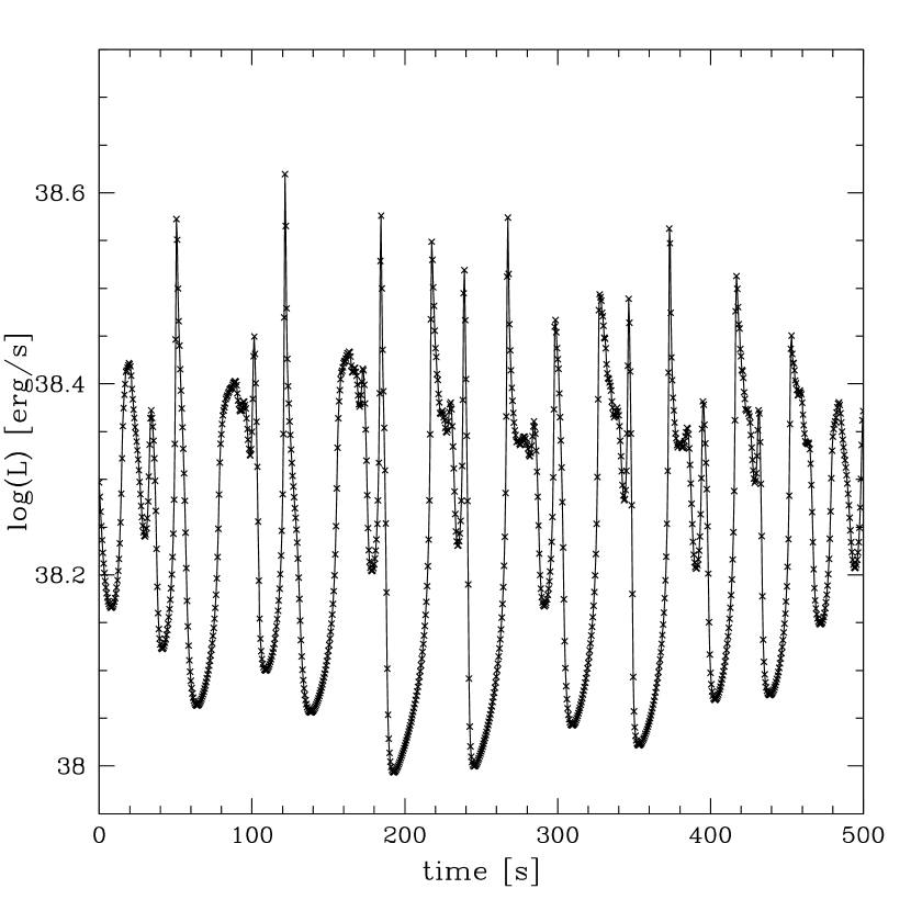
Figure 9: The disk lightcurve. Model parameters: $M=10M_{\odot}$, $\dot{m}_{\rm ext}=0.7$, $\alpha=0.01$. The fraction of the energy dissipated in the corona is $f_{\rm cor}=0.3$ and the outflow parameter is $A=0.075$.

In Figures 8 and 9 we show the luminosity curves for $\dot{m}_{\rm ext}=0.7$. In the first case the outflow was not included and the fraction of the energy dissipated in the corona was equal to $f_{\rm cor}=0.5$. This resulted in strong and regular outbursts. For the model with the outflow contribution parameterized by $A=0.075$ the outburst shape is quite irregular. In this case the share of the corona has been dropped to $f_{\rm cor}=0.3$, which allowed us to keep the mean outburst amplitude roughly unchanged.

Figure 10: Disk luminosity variations for different outflow and corona strengths. The open triangles mark solutions for corona parameter $f_{\rm cor}=0$, open squares for $f_{\rm cor}=0.1$, open circles for $f_{\rm cor}=0.2$, filled triangles for $f_{\rm cor}=0.3$, filled squares for $f_{\rm cor}=0.4$ and filled circles for $f_{\rm cor}=0.5$. Other model parameters were kept constant: $M=10M_{\odot}$, $\dot{m}_{\rm ext}=0.7$, $\alpha=0.01$.

In order to check if the luminosity variations would vanish for the largest outflow and corona shares, we computed a grid of models for the full range of these two parameters. Because the outflow creates irregular outburst shapes and amplitudes we parameterized the luminosity variations using the root mean square approximation, defined as:

$$rms={\sigma\over<L>},$$ (38)

where

$$\sigma^{2}={\int^{t_{2}}_{t_{1}}(L(t)-<L>)^{2}dt\over\Delta t},$$ (39)

$$<L>={\int^{t_{2}}_{t_{1}}L(t)dt\over\Delta t}$$ (40)

The time range $(t_{1},t_{2})$ was chosen arbitrarily and in our case it is $(1.4,1.41)\times 10^{5}$ sec, long enough to cover several outbursts for each of the studied lightcurves. In Figure 10 we plot the luminosity variations in terms of rms for different corona and outflow strengths. Both outflow and corona suppress the variations. Therefore the largest outbursts amplitude is achieved for disks with no corona and a very weak outflow, while the strong outflow and/or corona results only in luminosity “flickering”, which could be hardly detectable.

3.3.3 The disk thickness

The geometrically thin disk approximation is always satisfied in our model. However, during the outburst the inner parts of the disk become thicker than in the cold state (see Figure 11). This is because the temperature achieved during the outburs is controlled by the upper, advection supported branch of the stability curve.

Figure 11: The $H/R$ ratio during the disk evolution in the minimum (solid line) and maximum (dashed line) luminosity states. Model parameters: $M=10M_{\odot}$, $\dot{m}_{\rm ext}=0.7$, $\alpha=10^{-2}$. The corona share is $f_{\rm cor}=0.5$. The outflow is neglected.

3.3.4 Radiation spectrum

Figure 12: The disk blackbody spectrum in the minimum (solid line) and maximum (dashed line) luminosity states. Model parameters: $M=10M_{\odot}$, $\dot{m}_{\rm ext}=0.7$, $\alpha=0.01$. The corona share is $f_{\rm cor}=0.5$, but the power law tail is not plotted here. The outflow is neglected.

In Figure 12 we show the radiation spectra emitted by the accretion disk in the maximum (outburst) and minimum luminosity phases. We have made a simplifying assumption, that the disk radiates locally as a black body of temperature $T_{\rm eff}(r)$ and the resulting spectrum is integrated over the entire disk. We adopt the temperature distribution in the unstable region as that computed from our time dependent model, and we assume that the outside disk is stable and has a standard temperature distribution $T_{\rm eff}\sim r^{-3/4}$. The spectrum between the outbursts is a standard disk blackbody spectrum. However, when the disk becomes unstable, the radial temperature distribution is changed, which affects the spectral slope. Also, the maximum temperature is much higher, which causes the shift of the spectrum towards higher frequencies (see Zampieri et al. 2001). The presence of the corona and/or the outflow should add a power law component to the total spectrum, with an extension and slope appropriate for the hot plasma properties. This spectral component is not plotted in the figure.

4 Discussion

4.1 General properties of the model

The radiation pressure instability operating in the innermost parts of the accretion disk may be responsible for the periodical luminosity changes of a number of sources. The limit cycle behaviour produces outbursts with timescales and amplitudes which could reproduce the observed variability of Galactic black hols (on timescales of minutes) and short term variability of AGNs (on timescales of years), provided that certain assumptions about the model are satisfied.

In our time dependent calculations we use vertically averaged equations of the disk structure. Appropriate numerical coefficients need to be used in the vertical averaging, because they influence the critical accretion rate for which the limit cycle starts working. The description of the disk vertical structure also influences the computed outburst amplitudes, particularly in the case of the ’disk + corona’ model.

We calculated the time-dependent disk model and associated lightcurves and spectra assuming that a moderately strong corona extends above an accretion disk and contributes to the total accretion energy. Our assumption is consistent with the observed hard X-ray tail in the spectra and soft to hard X-ray luminosity ratios (e.g. Życki, Done & Smith 2001 for soft X-ray transients, Janiuk, Czerny & Madejski 2001 for the quasar PG1211+143). We also take into account the presence of the vertical outflow. These two assumptions let us obtain good agreement with the observed GBH lightcurves. For a bare accretion disk without a corona or an outflow, the outbursts are much too strong in respect to observations and the maximum luminosity exceeds the Eddington limit.

The outflow efficiency suppresses the maximum luminosity during the outburst. The luminosity reaches even 0.504 $L_{\rm Edd}$ in the case of no outflow (model with $f_{\rm cor}=0.5$), while for the outflow strength $A=0.01$ the luminosity drops to $0.2L_{\rm Edd}$ (for the same corona share). The total outflow power could in principle be as high as that emitted in the disk (Falcke & Biermann, 1999). Fender (2001) shows that the outflow is likely to be comparable in power to the integrated X-ray luminosity. In our calculations the outflow power is variable and depends on $L/L_{\rm Edd}$ ratio, achieving 30 - 70% of the observed disk luminosity during the outburst, for various sets of parameters.

Not only the outflow but also the corona reduces the outburst amplitude. If the fraction of energy dissipated in corona is small, a strong outflow is needed to suppress outbursts: in case of $f_{\rm cor}=0.1$ the outflow efficiency parameter has to be $A>0.25$. For $f_{\rm cor}=0.5$ only a small amplitude flickering ($\delta logL<0.05$) occurs when $A>0.05$. Here we adopt a simplified description of a corona, assuming constant coronal dissipation fraction $f_{\rm cor}$, but in general this parameter may depend on the radius (Janiuk & Czerny 2000). Recently, Merloni & Fabian (2002) proposed that the coronal fraction may drop for high accretion rates, being the most efficient in the low state of the source.

When either an outflow or a corona are strong enough ($f_{\rm cor}>0.55$ and/or $A>0.25$), the outbursts do not occur and the disk produces only flickering. Therefore these two mechanisms support each other and the stronger the corona the weaker outflow is required to suppress disk’s outbursts. We illustrate this correlation in Figure 13, where we show on the $A-f_{\rm cor}$ plane the parameter range for which we detect significant outbursts. Here the criterion for outburst detection was chosen that $rms>0.03$, that is the mean luminosity variations are above $\sim 5\%$ in logarithm.

The results strongly depend on the adopted external accretion rate. For small $\dot{m}_{\rm ext}$ the whole disk remains stable and the outbursts do not occur. However above a certain critical value the instability develops in the innermost disk part. The critical accretion rate above which outbursts are expected is $\dot{m}_{\rm ext}=0.28$ for a disk without a corona, but it increases to $\dot{m}_{\rm ext}=0.68$ when the corona shares 50% of the energy. This critical accretion rate does not depend on whether an outflow is present or not (see Figure 3). The amplitude of the outburst only weakly depends on the external accretion rate. Instead, the duration of the bursts increases strongly with $\dot{m}_{\rm ext}$, and the separation between the outbursts increases as well. For instance, for $\dot{m}_{\rm ext}=0.56$ the burst duration is $\delta t\sim 250$ seconds, while for $\dot{m}_{\rm ext}=0.39$ it is only $\delta t\sim 150$ seconds (model with no corona). It is the result of the enlarged instability region when the accretion rate is high.

The outburst amplitude is determined by the separation between $\dot{m}_{1}$ and $\dot{m}_{2}$, e.g. the lower and the upper turning points on the S curve (see Section 2.4). The point $\dot{m}_{1}$ is controlled mainly by whether the corona is present or not and how large is its contribution to the total accretion energy. The point $\dot{m}_{2}$ is influenced mainly by the strength of the outflow. In order to keep the outburst amplitudes no too high and not exceed the Eddington limit in the maximum luminosity phase, the point $\dot{m}_{2}$ must never be too high. In principle, the small value of $\dot{m}_{2}$ could alternatively be achieved by changing the viscosity parameter $\alpha$, and would not require any contribution from the hot wind. The variable viscosity may be parameterized e.g. by the disk thickness: $\alpha\sim(h/r)^{-n}$. However, we found that for low viscosities ($\alpha<10^{-3}$) the unstable radiation pressure dominated branch becomes too small for the instability to develop, and finally the disk achieves quasi-stable state in the intermediate range of temperatures (see Wallinder 1991).

In our model we assume the $\alpha$ viscosity prescription of Shakura & Sunyaev (1973). If the magneto-rotational instability was taken into account, the $\alpha$ parameter would also contain a magnetic contribution, which could slightly increase its effective value (Armitage et al. 2001). The qualitative results however should not be changed in this case. On the other hand, we assume a stationary material supply to the radiation pressure instability zone from the accretion disk regions outside $\sim 200R_{\rm Schw}$, while in principle additional instability mechanisms, such an ionization or gravitational instability, may play crucial role further out in the disk (Menou & Quataert 2001 and references therein).

Figure 13: Parameter range, for which the outbursts are expected. Model parameters: $M=10M_{\odot}$, $\dot{m}_{\rm ext}=0.7$, $\alpha=0.01$. The shaded region marks the corona and outflow parameters, for which the luminosity variations are greater than 5% ($rms>0.03$).

In all computed cases the duration of the outburst was significantly shorter (by a factor of 3 or more) than expected on the basis of the viscous timescale computed at the outer edge of the instability strip from the analytical formulae provided by Shakura & Sunyaev (1973). Therefore, numerical computations are needed to give appropriate viscous time scale estimates.

4.2 Application to GRS 1915+105

Observations of the microquasar GRS 1915+105 outbursts imply rather short time scales and low amplitudes of an outburst. Feroci et al. (2001) show lightcurves of the microquasar obtained by Beppo SAX. Typical soft X-ray band outbursts with $\Delta\log L\sim 0.6$ amplitude last for $\Delta t\sim 100$ sec. The disk luminosity in the outburst never exceeds Eddington luminosity. Therefore, based on our model, the whole limit cycle should run between $\dot{m}_{1}\sim 0.05$ and $\dot{m}_{2}\sim 1.0$.

The values of the transition accretion rates $\dot{m}_{1}$ and $\dot{m}_{2}$ (see Sections 2.4 and 4.1) depend significantly on the adopted description of the disk structure. In particular, the value $\dot{m}_{1}$ resulting from the model of Nayakshin et al. (2000) will be higher by a factor of 5 when the correct factors computed from the vertical structure model are included. It weakens significantly the motivation to postulate a strong coronal dissipation (up to 90% in Nayakshin et al. 2000) in this source, which is not observed but which served to increase $\dot{m}_{1}$ by a factor of 10. Therefore in our model we propose a moderately strong corona, dissipating 30-50% of the total energy. If the outflow takes away required amount of the total emitted power depending on the $L/L_{\rm Edd}$ ratio, the maximum observed disk luminosity should be lowered.

In our calculations we adopt the black hole mass equal to $10M_{\odot}$ (recent near infrared spectroscopy results indicate the mass of $14\pm 4M_{\odot}$, Greiner 2001) and constant viscosity parameter $\alpha=0.01$. With a corona dissipating $50\%$ of the total energy, no outflow, and external accretion rate equal to $70\%$ of Eddington rate the model results in strong and regular outbursts of $\Delta logL=0.7$ amplitude and timescales of $\Delta t\sim 140$ sec. If the outflow is present than the required by the observations corona is weaker and dissipates only $30\%$ of energy. In this case the theoretical lightcurve is quite irregular, with shorter and longer outbursts lasting for $\Delta t\sim 50-100$ sec and variable amplitudes of $\Delta logL\sim 0.3-0.7$.

The scenario of radiation pressure instability has one advantage over the disk evacuation scenario (Belloni et al. 1997b). As stressed by Rao, Yadav & Paul (2000), the rise/fall timescale during outbursts, $t\sim 10s$, is too short for a cold disk to be removed or reinstalled, as this should happen on a viscous timescale. In our model the whole accretion disk exists all the time, just its thermal state changes during outburst, with thermal timescale being short even for relatively high accretion rates. We see that clearly from Figure 2 of Janiuk, Czerny & Siemiginowska (2000) - rise and fall are much shorter than the duration of long outbursts typical for high accretion rates.

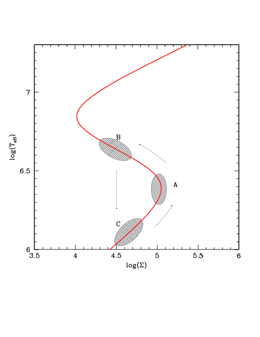
Figure 14: The hardness ratio states A, B, and C, defined as in Belloni et al. (2000), identified with the different positions of the disk on the stability curve. The curve is plotted for 10 $R_{\rm Schw}$. The cycle performed during the time evolution is marked by arrows.

Belloni et al. (2000) pointed out, that the source may occupy three distinct regions on the color - color diagram in X-rays. The colors are defined as $HR_{1}=F(5-13keV)/F(2-5keV)$ and $HR_{2}=F(13-60keV)/F(2-5keV)$. The state A corresponds to small values of both $HR_{1}$ and $HR_{2}$, state B is for $HR_{1}>1.1$ and small $HR_{2}$, while state C is for small $HR_{1}$ and large $HR_{2}$. The source alterations between states A, B and C are observed periodically, however the only one way transition between states B and C has been observed, namely from B to C, while the reverse transition has never happened. In our model we could identify the state C with the disk occupying the low stable branch of the S curve (see Figure 14), with a very soft disk blackbody emission and dominating power law component from the hot corona. The state A corresponds to the turning point on the stability curve, when the contribution of the disk blackbody emission is substantial, and state B refers to the unstable branch on the S curve. In the last case the emission from the hot disk is more pronounced in the X-ray spectrum. The disk normally evolves along the stability curve, going from C to A and further to B, or back to C state, depending on the accretion rate. However, when the disk reaches the unstable region B, the only possibility is to drop down to the state C, when the system finds the shortest possible way to come back to the stable solution.

4.3 Luminosity states in other sources and their relation to radiation pressure instability

Galactic black holes (GBH) exhibit a number of distinct luminosity states (van der Klis 1994, Poutanen, Krolik & Ryde 1997). Low (hard) state is characterized by a power law spectrum, with the photon index $\Gamma\sim 2$, and a complex variability. High (soft) state spectra are dominated by the disk emission, and the power spectrum is a simple power law with the index $\sim 1$ and a high frequency cut-off above 100 Hz. When the source gets brighter, in the Very High State, the spectrum is complex, with considerable and frequently variable contribution of the power law and disk emission, and the power spectrum shape is closer to the one in the hard state. Finally, the faintest sources represent a quiescent state.

Our model based on the radiation pressure instability predicts that the luminosity threshold exists and the disk becomes unstable when the luminosity exceeds this threshold. There is an important question to be put forward: are the Low, High and Very High states related in any way to the radiation pressure instability?

The theoretical luminosity threshold depends on the corona efficiency and varies from $0.28L_{\rm Edd}$ for no corona ($f_{\rm cor}=0$) to $0.68L_{\rm Edd}$ for $f_{\rm cor}=0.5$. The range of observed accretion rate corresponding to various luminosity states is rather difficult to assess. Firstly, only the luminosity in a restricted energy band is usually available, while estimates of the bolometric luminosity are reliable only if the data truly represent the broad spectrum. Secondly, there may sometimes be a confusion in the state definitions. The Very High State looks similar to both the hard state and the soft state, and it may be classified as one of those two, unless a careful analysis of both the spectral and temporal behaviour is performed. Keeping this in mind, we have collected a number of accretion rate estimates from the literature for the purpose of qualitative discussion. In Table 1 we show the estimates of the accretion rate (or luminosity to the Eddington luminosity ratio). Information is not complete since many states are observed mostly in transient sources and then the evolution may be too fast to collect many data (or sometimes even a single data set) for a given luminosity state.

There seem to be a large difference between the range of accretion rates in different states among various objects. Systematic errors and dispersion in inclination angles may partially be responsible for those observed differences, but there may also be some additional parameters hidden in the description of formation of the hot (coronal?) plasma. Still, sources are in their Low States when $\dot{m}\sim 0.05$, in the High States when $\dot{m}\sim 0.1$, and in the Very High States when $\dot{m}\sim 0.5$. The luminosity range corresponding to the High state is quite narrow, factor of 2 – 3 in accretion rate between the minimum and maximum value.

The Low and the High states are basically expected to be stable. The difference between these states does not seem to be related to radiation pressure instability but there must be a mechanism of hot plasma generation which works less efficiently when the total flux is larger. There are several phenomenological models proposed but the physics of formation and geometry of hot plasma is under discussion (e.g. Poutanen 2001, Di Salvo et al. 2001). Some objects in the High State are possibly slightly above the threshold predicted by our model although their coronal emission is not stronger than $f_{\rm cor}=0.5$ (LMC X-3 and J1748-288). It should be considered whether these sources are indeed in the High State, or rather in a disk dominated Very High State.

Sources in their Very High State are definitively in the range corresponding to the radiation pressure instability. Outbursts lasting a hundred to a thousand of seconds are expected. Such outbursts are however seen only in microquasars - GRS 1915+105 (see Sect. 4.2) and GRO J1655-40 (Remillard et al. 1999). The lack of outbursts in other sources is consistent with our model only if the corona and/or outflow are strong enough to suppress the instability completely. Since the ’corona’ (observationally - a power law component) in the Very High State contributes typically to about 30 % of energy, considerable outflow is also needed (parameter $A$ in our model of order of 0.2). In sources, which do not exhibit jets, the outflow must be uncollimated. The model does not include any description of the jet formation process, therefore it basically applies to such uncollimated outflow.

It remains to be checked whether this outflow is consistent with observations. Energetically, the request for such an outflow is plausible since the observed collimated jet may carry a considerable fraction of a total energy (Fender et al. 1999, Reeves et al. 2001). However, this material, if uncollimated, is in our line of sight and covers the disk, so part of the ’corona’ effect in the Very High State may be due to the Comptonization in this outflowing material. Such winds were also discussed in several contexts (e.g. wind driven instability of Shields et al. 1986, Beloborodov 1999, ADIOS models of Blandford and Begelman 1999). In the present model the wind should develop as a result of the disk instability, thus providing a stabilizing mechanism, and therefore it should cover only the radiatively unstable part of the disk. This hot wind plasma should have different properties than the hot coronal plasma formed in the Low state, which is probably produced by another mechanism.

Table 1: Luminosity ranges in Eddington units

Object	Very High State	High State	Low State	References
J1748-288	0.30 - 0.50	0.05 - 0.25	0.01 - 0.04	Revnivtsev et al. 2000
Nova Muscae	0.09 - 0.50	0.03 - 0.09	0.006	Życki et al. 1998
LMC X-3	$-^{b}$	0.07 - 0.3	$<0.07$	Wilms et al. 2001
Cyg X-1	$-^{b}$	$>0.03$	$<0.03$	Gierliński et al. 1997,
				Gierliński et al. 1999
GS 2023	$<1.6$	0.07	0.04 - 0.05	Życki et al. 1999 a,b
GRO J1615	0.2 - 0.25	0.1	$-^{a}$	Remillard et al. 1999,
				Gierliński et al. 2001
LMC X-1	$-^{b}$	0.15	$-^{b}$	Gierliński et al. 2001
GX 339-4	0.5	$-^{a}$	0.05 - 0.15	Miyamoto et al. 1995,
				Wilms et al. 1999
GRS 1915+105	$>0.15$	$-^{b}$	$-^{b}$	Zdziarski et al. 2001,
				Belloni 1997b
				Trudolyubov et al. 1999

4.4 The vertical outflow

In this work we postulate that a certain amount of the accretion energy is taken away by the vertical outflow. Since we do not include any collimation mechanism, this outflow has a form of a hot wind rather than a collimated jet, however its origin are the innermost regions of the accretion flow. We did not study this outflow in detail, since we took into account only the energy loss due to the wind. We neglected the mass loss and the effect of the hot flow onto the disk spectrum. However, we can estimate the properties of the outflowing wind a posteriori. The energy flux of the outflowing material is given by:

$$F_{\rm out}={1\over 2}\dot{m}_{\rm z}v_{\rm z}^{2},$$ (41)

where $v_{\rm z}$ is the outflow velocity in the vertical direction and $\dot{m}_{\rm z}$ is the mass loss rate. Therefore the outflow efficiency, defined by the Equation (25), is equal to:

$$f_{\rm out}={F_{\rm out}\over F_{\rm tot}}={4\pi r^{2}\dot{m}_{\rm z}\over 3\dot{M}f(r)}\times\big{(}{v_{\rm z}\over v_{\rm\varphi}}\big{)}^{2},$$ (42)

where local flux $F_{\rm tot}$ is given by Equation (4) and $v_{\rm\varphi}$ is the Keplerian velocity on the orbit $r$. Therefore the mass loss rate will be given by:

$$\dot{m}_{\rm z}={\dot{M}_{\rm Edd}A\dot{m}^{3}\over 4\pi r^{2}(1+A\dot{m}^{2})}\times\big{(}{v_{\rm\varphi}\over v_{\rm z}}\big{)}^{2}3f(r)$$ (43)

and may be negligible if e.g. $v_{\rm z}>3v_{\rm\varphi}$.

For the exemplary model with $A=0.1$, we set $\dot{m}\sim 1$ and $(v_{\rm\varphi}/v_{\rm z})^{2}\sim 0.1$ at $r=10R_{\rm Schw}$. The estimated density of the wind is then equal to $\rho_{\rm wind}=\dot{m}_{\rm z}/v_{\rm z}=2.7\times 10^{-9}$ g cm^-3. This means that the optical depth is of the order of $\tau_{\rm es}\sim 0.03$ and the outflowing medium should not have any substantial impact on the observed spectral properties of the X-ray source. The Comptonization in the wind may lead at most to the formation of a weak, steep power-law tail, additional to the disk black body emission. The X-ray reflection amplitude is also reduced by the bulk motion in the range of $\beta_{\rm bulk}\sim 0.6-0.7$, so this effect is practically negligible (Janiuk, Czerny & Życki 2000).

We stress that the uncollimated outflow which partially stabilizes the radiation pressure dominated disk is launched by a different mechanism than the jet seen in GRS 1915+105 during the prolonged C states. The latter is observed in the low luminosity intervals and is probably connected with the radio emission (Klein-Wolt et al. 2001).

5 Conclusions

Time dependent evolution of the inner accretion disk is based on the radiation pressure instability, playing major role in so called ’$\alpha$ disks’. This process accounts for a number of properties of Galactic black hole binary systems.

• The radiation pressure dominated innermost regions of the accretion disk are unstable and may oscillate between cold and hot phase. When the hot front goes through the inner disk, its surface density drops down rapidly by a factor of 3. As the disk cools down, it switches to the state of a relative faintness and the X-ray spectrum may be dominated by a power law emission from a hot corona. However, the disk is never evacuated completely and extends always down to the marginally stable orbit around a black hole.

• For high enough accretion rates ($\dot{m}>0.28$) and moderate strengths of the outflow and the corona, the instability results in a characteristic variability pattern, with 100 - 200 sec. outbursts of an amplitude reaching $\Delta logL\sim 0.3-0.7$. The irregular outbursts’ shape, observed in the microquasar GRS 1915+105, may result from the presence of the outflow, which takes away a high fraction of the energy when the disk luminosity is close to the Eddington limit.

• The presence of luminous outbursts and their amplitude depends on the assumed strengths of the disk corona and the outflow. These two elements may weaken the outbursts or even suppress them completely, therefore in most systems accreting at high $\dot{m}$ (observed in the Very High State) a rapid, large amplitude variability is not detected.

• The distinct regions occupied periodically by the microquasar on the X-ray color-color diagram correspond in our model to the characteristic phases during the time evolution. The theoretically predicted evolutionary track through these states: $C\rightarrow A\rightarrow B\rightarrow C$ explains the lack of $C\rightarrow B$ transitions. Observed transitions $B\rightarrow A$ and $A\rightarrow C$ and the fast X-ray flickering are not accommodated yet in the model, since they are both probably caused by hot plasma instabilities.

Acknowledgments. We thank Piotr Życki for helpful discussions. This work was supported in part by grant 2P03D00322 of the Polish State Committee for Scientific Research. AJ acknowledges support of the Harvard - Smithsonian Center for Astrophysics. This research was funded in part by National Aeronautics and Space Administration through Chandra Award Number GO1-2117B issued by the Chandra X-ray Observatory Center, which is operated by Smithsonian Astrophysical Observatory for and on behalf of the NASA under contract NAS8-39073.

References

- (1) Abramowicz M. A., Czerny B., Lasota J.-P., Szuszkiewicz E. 1988, ApJ, 332, 646
- (2) Agol E., Krolik J., Turner N.J., Stone J.M., 2001, ApJ, 558, 543
- (3) Alexander D.R., Johnson H.R., Rypma R.L., 1983, ApJ, 272, 773
- (4) Armitage P.J., Reynolds C.S., Chiang J., 2001, ApJ, 548, 868
- (5) Belloni T., Mendez M., King A. R., van der Klis M., van Paradijs J. 1997a, ApJ, 479, L145
- (6) Belloni T., Mendez M., King A. R., van der Klis M., van Paradijs J. 1997b, ApJ, 488, L109
- (7) Belloni T., Klein-Wolt M., Mendez M., van der Klis M., van Paradijs J., 2000, A&A, 355, 271
- (8) Beloborodov A.M., 1999, ApJ, 510, L123
- (9) Blandford R.D, Begelman M.C., 1999, MNRAS, 303, L1
- (10) Cannizzo J., 1993, ApJ, 419, 318
- (11) Cannizzo J., Chen W., Livio M., 1995, ApJ, 454, 880
- (12) Chen X. 1995, MNRAS, 275, 641
- (13) Di Salvo T., Done C., Życki P.T., Burderi L., Robba N.R., 2001, ApJ, 547, 1024
- (14) Dörer T., Riffert H., Staubert R., Ruder H., 1996, A&A, 311, 69q
- (15) Falcke H., Biermann P.L., 1999, A&A, 342, 49
- (16) Fender R., Garrington S.T., McKay D.J., Muxlow T.W.B., Pooley G.G., Spencer R.E., Stirlinge A.M., Waltman E.B., 1999, MNRAS, 304, 865
- (17) Fender R., 2001, Astrophysics and Space Science Supplement, 276, 69
- (18) Feroci M., Matt G., Pooley G., Costa E., Tavani M., Belloni T., 1999, A&A, 351, 985
- (19) Feroci M., Casella P., Costa E., Massaro E., Soffitta D., Matt G., Belloni T., Castro-Tirado A.J., Dhawan V., Frontera F., Harmon A., Mirabel I.F., Pooley G., Tavani M., 2001, Astrophysics and Space Science Supplement, 276, 15
- (20) Gierliński M., Zdziarski A.A., Done C., Johnson W.N., Ebisawa K., Ueda Y., Haardt F., Philips B.F., 1997, MNRAS, 288, 958
- (21) Gierliński M., Zdziarski A.A., Poutanen J., Coppi P., Ebisawa K., Johnson W.N., 1999, MNRAS, 309, 496
- (22) Gierliński M., Maciołek-Niedźwiecki A., Ebisawa, K., 2001, MNRAS, 325, 1253
- (23) Greiner J., to appear in Proceedings Jan van Paradijs Memorial Symposium, eds. E.P.J. Van den Heuvel, L. Kaper, E. Rol, ASP Conf. Series (astro-ph/0111540)
- (24) Hameury J.-M., Menou K., Dubus G., Lasota J.-P., Hure J.-M., 1998, MNRAS, 298, 1048
- (25) Honma F., Matsumoto R., Kato S. 1991, PASJ, 43, 147
- (26) Hure J.-M. 1998, A&A, 337, 625
- (27) Janiuk A, Czerny B., Siemiginowska A., 2000, ApJ, 542, L33
- (28) Janiuk A., Czerny B., 2000, New Astronomy, 5, 7
- (29) Janiuk A., Czerny B., Życki P.T., 2000, MNRAS, 318, 180
- (30) Janiuk A., Czerny B., Madejski G.M., 2001, ApJ, 557, 408
- (31) Klein-Wolt M., Fender R.P., Pooley G.G., Belloni T., Migliari S., Morgan E.H., Van der Klis M., 2001, MNRAS, in press (astro-ph/0112044)
- (32) Lightman A.P., Eardley D.M. 1974, ApJ, 187, L1
- (33) Lin D.N.C., Shields G.A., 1986, ApJ, 305, 28
- (34) Merloni A., Fabian A.C., 2002, MNRAS, 332, 165
- (35) Meyer F., Meyer-Hofmeister E., 1981, A&A, 104, L10
- (36) Meyer F., Meyer-Hofmeister E., 1984, A&A, 132, 143
- (37) Menou K., Quataert E., 2001, ApJ, 552, 204
- (38) Milsom J.A., Chen X., Taam R.E. 1994, ApJ, 421, 668
- (39) Miyamoto M., Kitamoto S., Hayashida K., Egoshi W., 1995, ApJ, 442, L13
- (40) Mineshige S., Shields G.A., 1990, ApJ, 351, 47
- (41) Mirabel I.F., Rodriguez L. 1994, Nature, 371, 46
- (42) Muchotrzeb B., Paczyński B., 1982, Acta Astron., 32, 1
- (43) Muschotzky R.F., Done C., Pounds K., 1993, Annu. Rev. A&A, 31, 317
- (44) Nayakshin S., Rappaport S., Melia F., 2000, ApJ, 535, 798
- (45) Paczyński B., Wiita P.J., 1980, A&A, 88, 23
- (46) Paczyński B., Bisnovatyi-Kogan G. 1981, Acta Asctron., 31, 283
- (47) Poutanen J., Krolik J., Ryde F., 1997, MNRAS, 292, L21
- (48) Poutanen J., 2001, Advances in Space Research, 28, 267
- (49) Pringle J.E., Rees M.J., Pacholczyk A.G. 1973, A.&A., 29, 17
- (50) Rao A.R., Yadav J.S., Paul B., 2000, ApJ, 544, 443
- (51) Reeves J.N., Turner M.J.L., Bennie P.J., Pounds K.A., Short A., O’Brien P.T., Boller Th., Kuster M., Tiengo A., 2001, A&A, 365, L116
- (52) Revnivtsev M.G., Trudolyubov S.G, Borozdin K.N., 2000, MNRAS, 312, 151
- (53) Remillard R. A. Morgan E. H., McClintock J. E., Bailyn C. D., Orosz Jerome A., 1999, ApJ, 522, 397
- (54) Różańska A., Czerny B., Życki P.T., Pojmański G., 1999, MNRAS 305, 481
- (55) Seaton M.J., Yan Y., Mihalas D., Pradhan A.K., 1994, MNRAS, 266, 805
- (56) Shakura N.I., Sunyaev R.A., 1973, A.&A., 24, 337
- (57) Shakura N.I., Sunyaev R.A., 1976, MNRAS, 175, 613
- (58) Shakura N.I., Sunyaev R.A., Zilitinkevich S.S., 1978, A&A, 62, 179
- (59) Shields G. A., McKee, C. F., Lin, D. N. C., Begelman, M. C., 1986, ApJ, 306, 90
- (60) Siemiginowska A., 1988, Acta Astron. 239, 289
- (61) Siemiginowska A., Czerny B., Kostyunin V., 1996, ApJ, 458, 491
- (62) Smak J. 1984, Acta Astron. 34, 161
- (63) Szuszkiewicz E., 1990, MNRAS 244, 377
- (64) Szuszkiewicz E., Malkan M.A., Abramowicz M.A., 1996, ApJ, 458, 474
- (65) Szuszkiewicz E., Miller J., 1997, MNRAS, 287, 165
- (66) Szuszkiewicz E., Miller J., 1998, MNRAS, 298, 888
- (67) Tanaka Y., Lewin W.H.G., 1995, in X-ray Binaries, eds. Lewin W.H.G., van Paradijs J., van den Heuvel E., CUP, Cambridge, p. 126-174
- (68) Taam R.E., Chen X., Swank J.H., 1997, ApJ, 485, L83
- (69) Trudolyubov S.P., Churazov E.M., Gilfanov M.R., 1999, Astronomy Letters, 25, 718
- (70) Turner N.J., Stone J.M., 2001, ApJS, 135, 95
- (71) Turner N.J., Stone J.M., Sano T., 2001, ApJ, 566, 148
- (72) Van der Klis M., 1994, ApJS, 92, 511
- (73) Yuan F., 1999, ApJ, 521, L55
- (74) Wallinder F.H., 1991, MNRAS, 253, 184
- (75) Wilms J., Nowak M. A., Dove J. B., Fender R. P., Di Matteo T., 1999, ApJ, 522, 460
- (76) Wilms J., Nowak M.A., Pottschmidt K., Heindl W.A., Dove J. B., Begelman M.C., 2001, MNRAS, 320, 327
- (77) Zampieri L., Turolla R., Szuszkiewicz E., 2001, MNRAS, 325, 1266
- (78) Zdziarski A.A., Grove J.E., Poutanen J., Rao A.R., Vadawale S.V., 2001, ApJ, 554, L45
- (79) Życki P.T., Done C. and Smith D.A., 1998, ApJ, 496, L25, 1998
- (80) Życki P.T., Done, C., Smith D., 1999a, MNRAS, 305, 231
- (81) Życki P.T., Done, C., Smith D., 1999b, MNRAS, 309, 561
- (82) Życki P.T., Done, C., Smith D., 2001, MNRAS, 326, 1367