Biases in Cometary Catalogues and Planet X

Abstract

Two sets of investigators – Murray (1999) and Matese, Whitman & Whitmire (1999) – have recently claimed evidence for an undiscovered Solar System planet from possible great circle alignments in the aphelia directions of the long period comets. However, comet discoveries are bedevilled by selection effects. These include anomalies caused by the excess of observers in the northern as against the southern hemisphere, seasonal and diurnal biases, directional effects which make it harder to discover comets in certain regions of the sky, as well as sociological biases. A simple mathematical model is developed to illustrate the geometrical selection effects controlling comet discoveries.

The stream proposed by Murray is shown on an equal area Hammer-Aitoff projection. The addition of newer data weakens the case for the alignment. There is also evidence that the subsample in the stream is affected by seasonal and north-south biases. The stream proposed by Matese et al. is most obvious in the sample of dynamically new comets, and especially in those whose orbits are best known. The most recent data continues to maintain the overpopulation in the great circle. This pattern in the data occurs with a probability of only $\sim 1.5\times 10^{-3}$ by chance. None of the known biases are able to provide such an alignment. Numerical integrations are used to demonstrate that a planet by itself can reduce the perihelia of comets in its orbital plane to sufficiently small values so that they could be discovered from the Earth. To maintain the observed flux of comets in the stream requires a parent population of $\sim 3\times 10^{9}$ objects on orbits close to the planet’s orbital plane.

There is a need for a sample of long period comets that is free from unknown or hard-to-model selection effects. Such will be provided by the European Space Agency satellite GAIA, which will discover $\sim 1000$ long period comets during its 5 year mission. This may finally bring to fruition the long tradition of looking for the effects of perturbers in cometary catalogues.

Figure 1: Upper panel: Plot of the aphelia of all 1A (squares) and 1B (triangles) comets in Marsden & Williams (1999) catalogue in heliocentric ecliptic longitude and latitude. Meridians of latitude are shown at $30^{\circ}$ intervals, parallels of longitude at $45^{\circ}$ intervals. The centre of the projection corresponds to the zero of longitude and is the first point of Aries. By convention, increasing longitude runs to the right, which is the mirror image of the sky as viewed by an observer on Earth. The solid line shows the projection of the Earth’s equator onto the celestial sphere. Lower panel: Plot of the aphelia of all (1A, 1B, 2A and 2B) comets discovered prior to 1940. The deficiency of comets with northern aphelia, especially at high latitude, is immediately apparent.

Discovery	Northern	Southern	Problematic	Problematic	Problematic	Total
Hemisphere	Perihelia	Perihelia	Probably North	Probably South
North	$71$	$17$	$10$	$12$	$13$	$123$
South	$6$	$17$	$1$	$2$	$2$	$28$

Table 1: Table showing discovery hemisphere versus hemisphere of perihelion passage for the 151 comets in Marsden & Williams (1999) which also appear in Vsekhsvyatskii (1964). The table demonstrates that comets passing perihelion in the celestial Northern hemisphere are preferentially discovered by observers in the terrestrial northern hemisphere, and vice versa. (Problematic comets are those difficult to classify either because they are closer than $15^{\circ}$ to the Sun at perihelion or because they pass perihelion on or near the celestial equator. If a tentative hemisphere of perihelion can be assigned to a problematic comet, we have tried to do so.)

1 Introduction

Since the discovery of Pluto, the idea that there may be an undiscovered tenth planet (Planet X) lying still further from the Sun has often been put forward. Attempts to predict the existence of undiscovered planets from studies of the aphelia of periodic comets have been made many times (e.g., Forbes 1880; Kritzinger 1957; Opik 1971; Guliev 1992). Most of these authors argued for a close planet at $\sim 50$ astronomical units (au). There is also work motivated by periodicities in the cratering and fossil records of $\approx 30$ Myr. Here, the idea is that the advance or the regression of the perihelion or aphelion of Planet X through the Kuiper Belt triggers periodic comet showers (e.g., Whitmire & Matese 1985; Matese & Whitmire 1986). Assuming Planet X is responsible for the periodicities, then it has a semimajor axis of typically $\sim 100$ au and a mass of a few Earth masses. A different hypothesis, motivated by the same periodicities, is a distant unseen companion to the Sun (Nemesis) on an eccentric orbit with semimajor axis $\sim 90000$ au and period $\sim 27$ Myr (Whitmire & Jackson 1984; Davis et al. 1984). The orbit has an assumed perihelion of $\sim 20000$ au, close enough to make incursions into the inner Oort Cloud and trigger comet showers (see Tremaine (1986), Vandervoort & Sather (1993), for reviews of the status of these theories).

The idea has most recently surfaced in this Journal in Murray (1999), who claimed first that the aphelia of long period comets between $30000$ and $50000$ show an excess and second that they are aligned along a great circle inclined at $\sim 30^{\circ}$ to the ecliptic. Murray interpreted this as evidence of the imprint of a body orbiting the Sun at $\sim 32000$ au with a period of $5.8\times 10^{6}$ years. Planet X is presumably massive (to produce a detectable family of comets) and its orbit is possibly retrograde, suggesting a recent capture by the Sun. A similar analysis was carried out by Matese, Whitman & Whitmire (1999), who looked at the same dataset of aphelia of long period comets. Matese et al. (1999) identified an excess of aphelia on a different great circle, this time with galactic longitude $\sim 135^{\circ}$, and argued that this must be produced by a bound perturber in the Oort Cloud. They suggested that there was a planet or brown dwarf with mass $\sim 3M_{\rm Jup}$ at $\sim 25000$ au on an orbit roughly normal to the Galactic plane. The distances suggested by Murray and Matese et al. for Planet X are in good agreement, but the comets that belong to the great circle streams are quite different in the two papers, as is the orientation of the orbit.

Even so, there is a some supporting theoretical evidence for Planet X. First, studies of the ejection and growth of planetesimals in the early Solar System do suggest the existence of a number of small planets beyond Pluto (e.g., Stern 1991, Kenyon & Luu 1999). Second, there are unexplained residuals in the motions of Uranus and Neptune, although it is difficult to evaluate the trustworthiness of the historical data (e.g., Anderson & Standish 1986, Hogg, Quinlan & Tremaine 1991).

In this paper, we analyse the evidence put forward by Murray (1999) and Matese et al. (1999). We begin with a thorough examination of the biases that afflict catalogues of long period comets in Section 2 and develop a mathematical model of the biases in Section 3 to illustrate our main points. Section 4 returns to the great circle alignments found by Murray (1999) and Matese et al. (1999) and assesses whether they are unexpected or not. Simulations are used to illustrate the possible signal of a massive perturber. In the concluding Section 5, we draw attention to the fact that the GAIA satellite will provide an all-sky catalogue of comets brighter than 20th magnitude and largely free of directional biases. We argue that this may finally bring to fruition the long tradition of looking for the effects of planets on the orbits of comets.

2 Observational Biases

Murray used the 1994 version, and Matese et al. the 1996 version, of the catalogue of long period comets by Marsden & Williams. Our data are extracted from the 1999 version. It is vital that the observational biases in this dataset be analysed before any great circle alignments can be accepted as real. In the past, a number of people have suggested possible effects (see e.g., Everhart 1967, Hughes 1983, Kresák 1983, Rüst 1984, Neslušan 1996), though a comprehensive treatment seems lacking.

2.1 North-South Biases

Marsden & Williams (1999) divide the long period comets into four classes, namely 1A, 1B, 2A and 2B, in order of diminishing certainty of the orbital elements. The upper panel of Figure 1 shows the aphelia of all 1A and 1B comets. This is an equal area Hammer-Aitoff projection using heliocentric ecliptic longitude and latitude coordinates. The bold line is the projection of the Earth’s equator onto the celestial sphere. It is evident from the figure that many more cometary aphelia lie to the south rather than the north of the projection of the Earth’s equator. Table 1 shows the raw statistics on perihelion passage as seen from Earth together with the hemisphere of discovery using comets from Marsden & Williams and data from Vsekhsvyatskii (1964). The table demonstrates that objects discovered in the north generally have perihelia in the north, and vice versa. Of course, there is a known excess of observers in the northern as against the southern hemisphere. So, this bias leads to a greater number of comets with aphelia in the southern rather than the northern hemisphere. Note that comets with perihelia within $\sim 30^{\circ}$ of the projected terrestrial equator may be discovered from either hemisphere. Hence, this bias is most pronounced in the sample of comets with high latitude aphelia. The lower panel of Figure 1 shows all comets (1A, 1B, 2A and 2B) in Marsden & Williams (1999) catalogue discovered prior to 1940. The bias in favour of southern aphelia is very pronounced, especially at high latitudes. This is expected because the excess of northern hemisphere observers relative to the southern hemisphere was greatest in the past.

Matese, Whitman & Whitmire (1998) contend that the north-south bias is minimized for comets whose orbits are well enough known. They argue that these comets are primarily bright. However, it could also be argued that, in order for a comet be studied enough for its orbit to be well known, it must be observed over a reasonable period of time, and that the excess of northern hemisphere observers again means that this is more likely to happen for comets with northern rather than southern perihelia.

Figure 2 shows a histogram of the number of comets in Marsden & Williams (1999) discovered per decade from the northern and southern hemisphere between 1810 and 1956, using the information in Vsekhsvyatskii’s (1964) book. This clearly shows the substantial bias towards northern hemisphere observers, which is still the case as late as the 1950s (the records in Vsekhsvyatskii’s book end in 1956). It even seems that the effects of great upheavals like the Boer War, the First World War and the Great Depression can be discerned in the diagram. However, statistics are low and so the passing interests of individual observers like Barnard, Perrine and Giacobini may also be a contributory factor. At first sight, it is surprising that there is not a dip during the Second World War. Looking at all single apparition long period comets in Vsekhsvyatskii (1964) gives us a larger sample than in the Marsden & Williams catalogue. We see that the number of comets discovered in five-year intervals from 1930 to 1950 by observers based in America rises from 3 to 4 to 5 to 7. For Southern Hemisphere observers, it changes from 3 to 2 to 6 to 13, while for observers based in Europe, it changes from 7 to 2 to 4 to 5. This suggests that the rise in discoveries from the United States and the Southern Hemisphere masks the deleterious effects of the Second World War on European discoveries. Similarly, plotting the cumulative total of numbered asteroids against time shows a steady, almost exponential increase, but there is a prominent plateau coinciding with the duration of the Second World War and ending in the 1960s. All this suggests that the cometary (and asteroidal) catalogues are not just telling us about astronomy!

Figure 2: Histogram of the number of comets discovered from the northern (solid lines) and southern (dotted lines) hemispheres in each decade prior to 1956. The comets are taken from Marsden & Williams (1999) catalogue, but the date of discovery and location of the discoverer are taken from Vsekhsvyatskii’s (1964) book.

Figure 3: Histogram of the number of comets against month of perihelion passage. This uses all comets (1A, 1B, 2A and 2B) in Marsden & Williams (1999) catalogue.

Figure 4: Plots of the aphelia of all comets (1A, 1B, 2A and 2B) in Marsden & Williams (1999) with perihelion passage in (a) May, (b) August, (c) November and (d) February. Meridians of ecliptic latitude are shown at $30^{\circ}$ intervals, parallels of ecliptic longitude at $45^{\circ}$ intervals. The centre of the projection is the zero of longitude and increasing longitude runs to the right. The solid line shows the projection of the Earth’s equator onto the celestial sphere. Notice (1) the north-south bias is most pronounced in northern winter months and (2) there is a zone of avoidance $\approx 180^{\circ}$ away from the position of the Sun (marked with a cross) as viewed from the Earth in panels (a), (b) and (d).

2.2 Diurnal and Seasonal Biases

There are a number of effects introduced into the catalogue of comets due to diurnal and seasonal bias. The time of day influences the area of the sky in which comets can be discovered. In general, a comet cannot be discovered until it is properly dark (after astronomical twilight), unless the comet is unusually bright or passes very close to the Sun. Similarly, if the comet is near opposition, it is further from the Sun than at quadrature, and is therefore harder to see. This suggests that the distribution of comet discoveries has a minimum towards the Sun and a secondary minimum towards midnight. All other things being equal, we expect there to be two equal maxima, one in the evening, and one in the morning, displaced towards midnight from the point of quadrature due to the effects of twilight. The seasons also impart a bias to the data, since the length of night varies, and hence there is more time to observe in winter, and therefore more objects will be discovered in winter than in summer. This can be seen to an extent in the raw numbers from the Marsden & Williams catalogue, which are plotted in Figure 3. However, the overall effect of this is probably reduced by the fact that the weather is generally worse in winter than summer at the temperate northern latitudes in which cometary observers predominate, which leads to a lowering in the number of observations made in winter. The most obvious feature in Figure 3 is a pronounced dip in mid-summer, along with peaks in April and August. Discoveries between August and April are roughly constant (bearing in mind that February is 10 % shorter than other months). The effects of the weather seem to counterbalance the effect of longer nights in these months.

Figure 4 shows plots of aphelia of comets which passed through perihelion in the months of May, August, November and February respectively. Ideally, these plots should show the comets discovered in each month. Unfortunately, the discovery months are scattered through the literature for post-1956 comets. So, we assume that the discovery took place close to perihelion. All the comets in Marsden & Williams (1999) catalogue are used. This seems reasonable because the direction of the perihelion in heliocentric coordinates should be fairly well-known, even if the detailed orbit is subject to uncertainties. The north-south bias is most pronounced in the northern winter months (see Figures 4 (c) and (d)). This is the coupled effect of the longer nights of the northern hemisphere winter, together with the excess of northern observers. By contrast, in Figures 4 (a) and (b), which correspond to the northern hemisphere summer months, there are very nearly equal numbers of comets with perihelia in each terrestrial hemisphere. The north-south bias of observers is almost cancelled by the longer nights of the southern hemisphere winter.

The panels in Figure 4 also show a zone of avoidance (marked with a cross) at longitudes $\approx 180^{\circ}$ away from the position of the Sun as viewed from the Earth. Comets cannot be discovered too close to the Sun. This means that comets with perihelia close to the Sun are unlikely to be discovered near perihelion. Holetschek (1891; see also Hughes 1983) pointed out a similar effect – namely, that comets with perihelion the far side of the Sun are less likely to be discovered both because of the proximity of the Sun and because they are further away and hence fainter. In May, the zone of avoidance is centered at an ecliptic longitude of $\approx 225^{\circ}$ and advances by $90^{\circ}$ as we move forward by three months. The zone is obvious in the May, August and February plots, although not at all in the November plot. Figure 5 shows the aphelia of comets which passed through perihelion in the month of July. It is included because the zone of avoidance is very clearly seen opposite the Sun at ecliptic longitudes of $\approx 285^{\circ}$. Even more strikingly, the region of sky above $30^{\circ}$ north of the ecliptic is completely devoid of all cometary aphelia. This is strong evidence that even in summer, the smaller numbers of southern observers are affecting the results. Another effect that is visible in the July and August plots is a tendency for comets to cluster about the apparent position of the Sun. These are comets with perihelia outside the Earth’s orbit discovered near opposition and possibly near perihelion. A northern hemisphere observer at this time of year has a comparatively small area of sky to search, due to the short summer nights. This biases cometary discoveries to the area around opposition, which explains the apparent clustering.

There is another diurnal effect that has been suggested in the literature. As is well-known, many more meteoroids are observed in the morning as compared to the evening (e.g., McKinley 1961). We encounter many more meteoroids on the forward side of the Earth, and those encountered are also brighter as they have a higher relative velocity. By contrast, in the evening the meteoroids have to catch up the motion of the Earth and so are scarcer and fainter. By analogy, Kresák (1983) suggested that such a diurnal asymmetry may be present in cometary discoveries. This, however, is not clear, as comets are not discovered through encounter with the Earth and so relative velocities do not appear to be important. Kresák’s bias may have been important in the days of naked eye discoveries, as comets that have passed through perihelion are often brighter. This may have biased statistics towards the discoveries of retrograde comets in the morning.

Figure 5: Plot of the aphelia of all comets (1A, 1B, 2A and 2B) in Marsden & Williams (1999) with perihelion passage in July. The solid line shows the projection of the Earth’s equator onto the celestial sphere. Notice (1) there are no aphelia above an ecliptic latitude of $30^{\circ}$ North and (2) the zone of avoidance is evident at an ecliptic longitude of $\approx 285^{\circ}$ (marked with a cross).

2.3 Directional Biases

There is a bias against areas of the sky with high stellar densities or dense nebulosity. The crowded nature and high surface brightness of such areas makes it harder to discover a comet against the background. Hence, we might expect a dearth of cometary discoveries, for example, in the plane of the Milky Way. However, there may be other subtle effects operating, since some areas of the sky are of much greater interest to observers than others. If an area of sky is receiving twice the attention of a neighbouring area, we might assume that the better observed area will yield a greater number of comet discoveries. An interesting example of a recent comet discovered in a region with a dense stellar background is Comet Hale-Bopp (C/1995 O1). This was found independently by Hale and Bopp, who were observing the globular cluster M70 in the direction of Sagittarius (see IAU Circular 6187). The comet just happened to lie in the same field of view.

Another directional bias comes from groups of comets that fragmented at a perihelion passage prior to discovery. The aphelia of such objects will form a tight cluster. The most obvious example is the Kreutz family of sun-grazing comets (see e.g., Marsden 1989). There are 3 Kreutz family sun-grazers in the catalogue of osculating elements of Marsden & Williams (namely, C/1882 R1-B, C/1963 R1, C/1965 S1-A). These can be seen in the upper panel of Figure 1 as the three superposed symbols at an ecliptic longitude of $\approx 130$ degrees.

Finally, directional biases may also come from showers of comets produced by weak stellar perturbations of the Oort Cloud. For example, Biermann, Huebbner & Lüst (1983) pointed out that there is a surplus of cometary aphelia in the region bounded by $180^{\circ}\mathrel{\hbox to0.0pt{\lower 3.0pt\hbox{$\sim$}\hss}\raise 2.0pt\hbox{$<$}}\ell\mathrel{\hbox to0.0pt{\lower 3.0pt\hbox{$\sim$}\hss}\raise 2.0pt\hbox{$<$}}240^{\circ}$ and $0^{\circ}\mathrel{\hbox to0.0pt{\lower 3.0pt\hbox{$\sim$}\hss}\raise 2.0pt\hbox{$<$}}b\mathrel{\hbox to0.0pt{\lower 3.0pt\hbox{$\sim$}\hss}\raise 2.0pt\hbox{$<$}}30^{\circ}$, where ($\ell,b$) are galactic longitude and latitude. They attributed this to this to an encounter with a roughly solar mass star 3 Myrs ago. Irrespective of whether the details of the explanation are correct, the shower does seem to be a real dynamical effect, as it is more prominent in the more tightly bound comets (e.g., Matese et al. 1999). Further weak showers may remain undetected in the dataset.

2.4 Orbital Biases

Of course, comets do not all have an equal chance of discovery, as some orbits offer more favourable opportunities. It is well known that most comet searchers concentrate their efforts close to the plane of the ecliptic, and so high inclination comets are under-represented in catalogues. The bias towards low inclinations in long period comet catalogues is still further enhanced by contamination of the sample with misclassified short period comets. Comets with very small perihelion distances spend less time in the inner solar system than those at large perihelion distances and cover a much smaller arc. They are hence more likely to be missed, unless they are bright enough to be seen when very close to the Sun. Similarly, objects with large perihelion distance will be observable on a large arc. Comets with perihelia lying noticeably beyond the Earth’s orbit will be most favourably placed for discovery at opposition rather than at perihelion passage. Comets with perihelia the far side of the Sun are less likely to be discovered both because of the closeness of the Sun and because they are further away and fainter (the Holetschek effect mentioned in Section 2.2).

Comets with both high inclination and small perihelia offer particular difficulties. For example, if the the perihelion is in the north, then the comet spends most of its observable time in the southern hemisphere and may well be too close to the Sun at perihelion to be observed from the north. Table 1 demonstrates that comets tend to be discovered in the same hemisphere as the perihelion passage, but this is not true for for comets with small perihelia ($\mathrel{\hbox to0.0pt{\lower 3.0pt\hbox{$\sim$}\hss}\raise 2.0pt\hbox{$<$}}0.2$ au).

Finally, objects in outburst are unpredictable and may be discovered at large heliocentric distances. Unusually bright and large comets, such as Hale-Bopp, are likely to be discovered a long time before perihelion passage. Comets are known to be much more active when new and fade on subsequent apparitions, presumably because the most volatile components are substantially lost at the first perihelion passage leading to a dimming of the intrinsic brightness thereafter. So, first time entrants from the Oort Cloud over the past 200 years (the time over which records have been maintained) are more likely to have been discovered than comets which were returning for a second or third time during the same period.

2.5 Sociological Biases

The heart of the problem is the uneven coverage of the sky at different epochs by different generations of observers. We have already suggested in Section 2.1 that the effects of historic upheavals like the First World War and the Great Depression may be able to be discerned in cometary catalogues. There may be additional effects that are sociological in origin. For example, especially in observations from casual observers, there may be an additional time of day bias. Many casual observers prefer to observe in the evening before going to bed, rather than in the morning after rising. Due to the difference in weather in winter and summer, casual observers in the northern hemisphere would perhaps rather observe in the warm summer months, which may slew the seasonal observations towards the months after the summer solstice. This is in accord with Figure 3, which shows that August is the best month for cometary discoveries.

2.6 Biases with Survey Programmes

Since 1999, the overwhelming majority of comets have been discovered by search programmes, such as LINEAR (“http://www.ll.mit.edu/LINEAR/”) and NEAT (“http://neat.jpl.nasa.gov/”). For example, 14 of the last 20 comets in the catalogue of Marsden & Williams were discovered by LINEAR and a further 2 comets were found by NEAT. It is apparent, given the success of these programmes, that in the future such surveys will constitute the overwhelming bulk of discoveries. The days of comet discoveries by amateur observers are drawing to a close. The surveys evade some of the biases above, but they introduce their own selection effects. One bias immediately obvious is that both LINEAR and NEAT are situated in the northern hemisphere. Neither will discover comets in the far south of the sky. This is the same situation as was present for visual observers in the past – a north-south bias is introduced into the dataset due to the observers rather than any astronomical effect. In addition, it appears from the skyplots of observations made by LINEAR that the area around the North Celestial Pole is not observed and so this area will show a dearth of discoveries. Another bias is that the survey telescopes only operate during ’dark time’. So, the periods around full moon will not be covered by the telescopes. This means that comet discoveries will by bunched away from periods of moonlight to a greater extent than in the past.

2.7 Anisotropies

Finally, there have been repeated claims of anisotropies in the aphelia directions (e.g., Yabushita 1979). The preferred direction has typically been found to coincide closely with the solar antapex. This played an important role historically as it was one of the pieces of evidence that was thought to favour Lyttleton’s (1953) accretion theory of cometary origin. The strength and direction of any anisotropy can be quantified by harmonic analysis. This idea is familiar in cosmic ray physics (e.g., Linsley 1975; Evans, Ferrer & Sarkar 2002), although apparently has not been used before in cometary science. Let ($\lambda,\beta$) be heliocentric ecliptic coordinates and

$$N=\sum_{i}h(\lambda_{i},\beta_{i}).$$ (1)

The Fourier coefficients are

$$a=\frac{2}{N}\sum_{i}h(\lambda_{i},\beta_{i})\cos\lambda_{i},\quad b=\frac{2}{N}\sum_{i}h(\lambda_{i},\beta_{i}){\sin\lambda_{i}},$$ (2)

where the index $i$ runs along all the comets in the sample and $h(\lambda,\beta)$ is the selection function. The amplitude $R$ and phase $\psi$ of the first harmonic is

$$R=(a^{2}+b^{2})^{1/2},\qquad\psi={\rm atan}\Biggl{(}{b\over a}\Biggr{)}.$$ (3)

The probability that an amplitude higher than that measured $R$ can arise from an underlying isotropic distribution is given by the formula (Linsley 1975)

$$P(>R)=\exp(-k_{0}),\qquad k_{0}=\frac{1}{4}R^{2}N.$$ (4)

The selection function $h(\lambda,\beta)$ is both important for analysing any alleged anisotropies and nearly impossible to model. It is reasonable to argue that the cometary data accumulated over long periods of time is reasonably independent of biases in ecliptic longitude. A crude way to cope with the north-south bias is to split the cometary sample into those with aphelia in the northern or southern ecliptic hemispheres, and to analyse each sample separately.

Dataset	$N$	$R$	$\psi$	$P(>R)$
Northern aphelia	$136$	$0.364$	$44.2^{\circ}$	$0.011$
Southern aphelia	$194$	$0.228$	$-84.9^{\circ}$	$0.080$
All	$330$	$0.257$	$68.1^{\circ}$	$0.004$

Table 2: Tests for isotropy on the cometary aphelia dataset. Results are given for the whole sample, as well as for the subsamples with aphelia in the northern ecliptic and southern ecliptic hemispheres. The second column gives the number of comets $N$. The third and fourth columns give the amplitude and phase, while the fifth gives the probability that an isotropic distribution could give an amplitude greater than that observed $R$.

This is performed in Table 2 for all comets in Marsden & Williams catalogue, as the the direction of the aphelion in heliocentric coordinates should be fairly well-known, irrespective of the other orbital uncertainties. The final column of Table 2 shows that the probability of an isotropic distribution yielding such large values of the amplitude $R$ is small. From the results of Jaschek & Vabousquet (1994), the solar antapex lies in the direction $\lambda=88.3^{\circ}$, $\beta=-49.9^{\circ}$ (using equinox 2000). The longitude lies within $\approx 20^{\circ}$ of the phase found by the anisotropy analysis of the whole sample. However, the phase does not point in a consistent direction for the three samples (comets with northern aphelia, with southern aphelia and the entire dataset) and hence, it seems that any correlation of anisotropy with the antapex direction is untrustworthy.

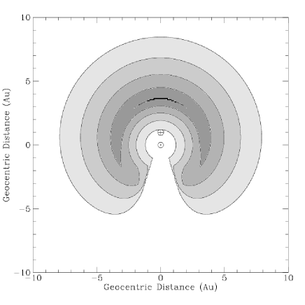
Figure 6: Contour levels of the relative probability of discovery of a comet in the plane of the ecliptic. The positions of the Sun and the Earth are marked. The contours are spaced at intervals of relative probability of 0.2, with the highest level (the darkest) being unity. The plot is drawn for a comet with absolute magnitude $H_{0}=5$ and power-law index $n=2$, together with an assumed extinction of 0.25 magnitudes per airmass. Such a comet is five times more likely to be discovered within the very dark crescent-shaped region than within the lightest grey horseshoe-shaped region.

Figure 7: Plot of the relative discovery probability integrated along the line of sight. Here, $\theta$ is measured relative to the Earth-Sun line. In the left-hand plots, the results are shown as polar plots with the length equal to the relative probability, whereas the right hand plots are graphs of relative probability against $\theta$. The upper and lower panels refer to a bright comet ($H_{0}=0$) and faint comet ($H_{0}=10$) respectively. Note that for faint comets the distribution has a minimum towards the Sun and a secondary minimum at midnight.

3 A Model of Discovery Probability

In this Section, we illustrate some of the biases with a simple model. Let us denote the relative probability of discovery of a comet at any heliocentric position ${\bf r}$ as $P({\bf r})$. This is equal to the relative probability ${P_{\rm loc}}({\bf r})$ that there is a comet at the location ${\bf r}$ multiplied by the probability $P_{\rm obs}({\bf r})$ that a comet at ${\bf r}$ will actually be observed.

3.1 The Algorithm

We assume that all comets move on parabolae and that the cometary perihelia occur uniformly in space about the Sun. The orientation of the orbit is completely specified if the rotation angle of the parabola about the major axis is given. We assume that this angle is distributed uniformly between $0^{\circ}$ and $360^{\circ}$. We assume that comets are discovered at random time intervals within 10 months either side of the perihelion passage. For each cometary arc, we pick a random time $t$ and solve for the true anomaly $v$ using (e.g., Danby 1992, p. 130)

$${1\over 3}\tan^{3}\left({v\over 2}\right)+\tan\left({v\over 2}\right)={kt\over\sqrt{2q^{3}}},$$ (5)

where $k$ is the Gaussian gravitational constant and $q$ is the perihelion distance. This is used to give the heliocentric distance $r=|{\bf r}|$ at time $t$ through

$$r={q\over 1+\cos v}.$$ (6)

This heliocentric position corresponds to two points on the orbit, symmetrically placed before and after perihelion. The same probability is allocated to each of these points. By generating $\sim 10^{6}$ such trials in Monte Carlo fashion, we find that the relative probability of a comet being at a position $r$ from the Sun is

$${P_{\rm loc}}({\bf r})={\rm min}(0.15r^{3/2},1).$$ (7)

The numerical pre-factor ($0.15$) varies only slightly as the window of discovery about the perihelion point is changed. An intuitive explanation of the power-law dependence with radius is that it is a consequence of Kepler’s Third Law. The larger the heliocentric distance, the more slowly a comet moves, and so the relative probability ${P_{\rm loc}}$ eventually reaches a plateau.

Let $\theta$ be the angle between the comet and the Sun as seen from the Earth. If $\theta<18^{\circ}$, then the comet has set before the end of astronomical twilight. We assume that objects so close to the Sun are undetectable. If $\theta=102^{\circ}$, then the comet is overhead at the end of nautical twilight. When $102^{\circ}<\theta\leq 180^{\circ}$, then the comet is directly overhead some part of the Earth’s globe during the night. Of course, the airmass is unity when the comet is overhead. If $18^{\circ}<\theta<102^{\circ}$, then the minimum extinction is calculated by working out the highest the object can be in the sky under dark conditions. This is the zenith angle $z=102^{\circ}-\theta$. The definition of airmass $a$ is

$$a={1\over\cos z}.$$ (8)

When $z<30^{\circ}$, then the airmass is computed from the slightly more accurate formula (e.g., Kristensen 1998)

$$a=\sqrt{0.635\cos^{2}z+2.954}-0.79\cos z.$$$$ (9)

The apparent magnitude of the comet is

$$m=H_{0}+5\log\Delta+2.5n\log r+(a-1)\epsilon.$$ (10)

Here, $r$ is the heliocentric and $\Delta$ the geocentric distance of the comet, while $n$ is the “power law exponent”, which determines how rapidly the object brightens when it comes close to the Sun, and $H_{0}$ is the absolute magnitude (the magnitude at 1 au from Sun and Earth and zero phase angle). The quantity $\epsilon$ is the number of magnitudes of extinction per airmass, which is taken as $0.25$ in our calculations. From the apparent magnitude, we assign the probability of observation as follows.

$$P_{\rm obs}=\cases{1&if $m<10$,\cr(15-m)/5&if $10<m<15$,\cr 0&if $m>15$.}$$ (11)

In other words, if the comet is fainter than 15th magnitude, we assume that it is not observed. If the comet is brighter than 10th magnitude, the probability is unity. Between 10 and 15, the probability falls off in a linear manner. Of course, these choices are somewhat arbitrary, but they are a reasonably realistic simplification of a complex issue. Obviously, the limiting magnitudes are chosen to represent typical conditions over the last 200 or so years of comet searching.

Figure 8: Plot of the relative discovery probability integrated both along the line of sight and over the luminosity functions given in eq (12) (upper panels) and eq (13) (lower panels). The maximum of each graph has been normalised to unity. Note that the secondary minimum at midnight is enhanced as compared to Figure 7, as both LFs are dominated by faint objects.

Figure 9: Plot showing how discovery probability as a function of direction varies with the season. For a northern hemisphere observer, the probability of discovering a comet at southerly declinations is greatest in winter rather than summer.

3.2 Results

The observation probability $P_{\rm obs}$ multiplied by the location probability ${P_{\rm loc}}$ gives the relative probability that a comet is discovered at a given location. Figure 6 shows the probability distributions for a typical comet ($H_{0}=5$). The figure is plotted in the plane of the ecliptic and can be rotated about the Sun-Earth line to give the full three-dimensional plot. The opening angle of the two lobes is $36^{\circ}$, which is a consequence of the assumption that no comets are discovered if they are so close to the Sun that they set before the end of astronomical twilight. The curvature of the lobes in the Sun-ward direction is controlled by the amount of extinction – the larger the extinction, the less likely an object is to be discovered at high airmass and the squatter the distribution. The overall size of the contours is set by the absolute magnitude and power-law index of the comet. Figure 7 shows the probability integrated along the line of sight as a function of the observed angular separation of the comet from the Sun. The left panels show a polar and the right panels a graphical representation of the results for a very faint ($H_{0}=15$) and very bright ($H_{0}=0$) comet. For a comet with such characteristics, these diagrams show the most likely angle of discovery. Note that – as anticipated in Section 2.2 – the distribution has a minimum towards the Sun and a second minimum at midnight. This effect is most obvious in the very faint comets, as bright comets can be discovered at greater heliocentric distances.

These figures hold good for observers on or close to the Earth’s equator (at latitudes $\mathrel{\hbox to0.0pt{\lower 3.0pt\hbox{$\sim$}\hss}\raise 2.0pt\hbox{$<$}}30^{\circ}$). As we move off the equator, two things happen. First, the angle at which the Sun sets varies from the vertical at the equator to the horizontal at the poles. For an object to be discovered at the poles, it would have to lie at a declination $18^{\circ}$ or more to the north of the Sun. The effect of this is to vary the opening angle of the lobes. Second, the length of night and hence the maximum distance of the Sun beneath the horizon also vary over the course of the year. Again, the extreme is at the poles, which experience $\sim 183$ days of daylight followed by $\sim 183$ days of night. This causes the overall size of the figure to shrink or expand depending on the season.

So far, our analysis is appropriate for comets with a given value of $H_{0}$ and $n$. To provide results for an ensemble, we must integrate over the luminosity functions (LFs). We examine two LFs, the first being a simple power-law magnitude distribution (e.g., Hughes 2001)

$$dN\propto 2^{H_{0}}dH_{0},\qquad\qquad\qquad\qquad-3<H_{0}<15.$$ (12)

Here, $dN$ is the number of comets with intrinsic brightnesses in the interval $H_{0}$ to $H_{0}+dH_{0}$. The second is the improvement suggested by Hughes (2001), namely

$$dN\propto 10^{-2.607+0.359H_{0}}dH_{0},\qquad\quad-3<H_{0}<15.$$ (13)

Of course, both these laws are over-simplifications and we have extended them to magnitudes fainter than their limits of known validity. Nonetheless, this is justifiable as we are interested in understanding the qualitative effects of the increasing number of objects at faint magnitudes. Comet Sarabat of 1729 is thought to have had an absolute magnitude of -3 (e.g., Vsekhsvyatskii 1964), whilst the faintest comets considered by Hughes have an absolute magnitude of $\approx 15$. So we use these as our magnitude limits. Figure 8 shows the result of integrating over the LFs. The results are very similar, irrespective of whether the LF given by eq (12) or eq (13) is used. Both LFs are dominated by faint comets and so the secondary minima are very pronounced. This result is robust against quite drastic alterations in the LF.

Finally, Figure 9 illustrates the effects of the seasons. The position of the Earth is shown relative to the Sun at the equinox and at the summer and winter solstices. The position of the lobes stays constant with respect to the Earth-Sun line, which causes them to appear to rock in declination against the background sky to an Earth-bound observer. From the diagram, we can see that for a northern hemisphere observer, the probability of discovering a comet at southerly declinations is greatest in winter rather than summer.

Figure 10: The upper panel shows all 1A (squares) and 1B (triangles) comets satisfying Murray’s (1999) criteria in an equal area Hammer-Aitoff projection. The centre of the projection corresponds to the zero of ecliptic longitude. Meridians of ecliptic latitude are shown at $30^{\circ}$ intervals, parallels of ecliptic longitude at $45^{\circ}$ intervals. The lower panel shows the data in a form similar to that originally presented by Murray (1999), together with the best fit sine curve to those comets identified by Murray as objects on their first return after temporary capture by Planet X. Note that Murray’s original plot included only the 1A comets in the 1994 version of Marsden & Williams.

Name	q	$10^{6}/a$	$b$	$\ell$	$\beta$	$\lambda$	Discovery
C/1925 G1	1.109477	+40	10.9	238.8	-35.5	131.9	Apr
C/1946 P1 *	1.136113	+44	-19.7	127.2	32.3	34.1	Aug
C/1989 Y1 *	1.569172	+49	-6.6	329.2	-35.3	255.2	Dec
C/1888 R1 *	1.814916	+48	59.2	314.9	4.5	198.0	Sep
C/1932 M2 *	2.313581	+45	-14.1	146.9	24.4	54.6	Aug
C/1973 A1	2.511124	+49	-50.6	107.3	9.0	6.3	Jan
C/1983 O1 *	3.317899	+48	54.7	325.3	4.4	205.2	Jul
C/1987 F1 *	3.624588	+59	-26.2	130.4	25.2	33.0	Mar
C/1954 O2	3.869934	+42	-18.9	336.6	-34.7	272.6	Aug
C/1979 M3	4.686916	+42	14.6	207.4	-10.1	112.7	Aug
C/1987 H1	5.457548	+46	-17.0	191.2	-12.5	76.7	Apr
C/1976 D2 *	6.880674	+59	-44.2	121.8	12.4	17.7	Feb
C/1886 T1	0.663317	+46	-24.5	288.7	-77.8	246.6	Oct
C/1912 R1	0.716079	+45	13.0	225.9	-25.2	123.1	Sep
C/1900 B1 *	1.331529	+57	42.1	305.5	-13.2	201.1	Feb
C/1937 C1	1.733791	+62	-38.7	214.7	-39.2	61.7	Feb
C/1990 M1	2.682238	+40	-48.4	172.0	-13.2	40.6	Jun
C/1997 J2	3.051136	+40	-0.4	261.4	-57.3	150.8	May
C/1960 M1	4.266927	+40	-12.3	221.2	-36.2	95.9	Jun
C/1999 F2 *	4.718792	+57	-45.7	136.2	6.3	26.1	Jun
C/1993 F1	5.900474	+59	-45.5	330.2	-45.5	305.4	Mar

Table 3: Data on all 1A and 1B comets satisfying Murray’s (1999) criteria. Murray considers only the 1A comets are known well enough to qualify for membership of the great circle stream. The 12 comets in the upper table were used in his original work. The 9 comets in the lower table include 2 new 1A comets (C/1997 J2 and C/1993 F1) and 7 1B comets. The table lists perihelion $q$, the reciprocal of the semimajor axis $1/a$, galactic longitude and latitude ($\ell,b$), ecliptic longitude and latitude ($\lambda,\beta$) and month of discovery. All distances are in au and all angles in degrees. (Objects with an asterisk also occur in Matese et al.’s (1999) stream as well.)

Figure 11: Plot of orbital period against ecliptic longitude for the 1A (squares) and the 1B (triangles) comets in Table 3. The dashed line shows the longitudinal trend of cometary period suggested by Murray (1999).

4 Great Circle Alignments

Both Murray (1999) and Matese et al. (1999) claimed the detection of (different) great circle alignments in the aphelia of the long period comets. In this section, we sift the evidence that they presented with an eye as to whether biases and selection effects could have caused the suggested alignments.

4.1 The Planet of Murray

First of all, Murray (1999) argued that there is an excess of aphelia of long period comets in the range 30000 to 50000 au and that this may be a piece of evidence for an undiscovered planet. An immediate worry is that for objects with aphelia $\mathrel{\hbox to0.0pt{\lower 3.0pt\hbox{$\sim$}\hss}\raise 2.0pt\hbox{$>$}}10000$ au, the eccentricity is close to unity. Therefore, small errors in the eccentricity can cause substantial errors in the value of $1/a$ and hence in the aphelion distance. In the osculating elements catalogue of Marsden & Williams (1999), there are comets classified as 1A which are nominally hyperbolic prior to their entry into the Solar System. The most extreme example is C/1996 J1-a which has a values of $1/a$ of $-0.000511$. Even allowing for the fact that this is an unusual object, it is clear that the typical errors in the value of $1/a$ are sufficient to move cometary aphelia by $\sim 10000$ au at these distances. Another worry is that a maximum in the distribution of aphelia seems to arise quite naturally. Just from considerations of spatial volume alone, the number of comets with aphelia in the range [$Q,Q+dQ$] is expected to be an increasing function of $Q$. In the inner areas of the Oort Cloud ($\sim 10^{3}-10^{4}$ au), it is reasonable to assume that very few comets will be ejected from the Cloud by the passage of nearby stars and perturbations from the Galaxy. The further from the Sun, the more powerful are the effects of these ejection mechanisms and so the lower the probability of any individual comet surviving for the current age of the Solar System. Hence, in the outer parts of the Cloud, the number of comets with aphelia in the range [$Q,Q+dQ$] is expected to be a decreasing function of $Q$. It is apparent from the two competing effects that a turnover or maximum in the number of long period comets as a function of aphelion distance is inevitable and that this maximum could well occur in the range 30000 to 50000 au.

Figure 10 shows all 1A and 1B comets fulfilling Murray’s criteria (namely, with aphelia between 30000 and 50000 au) in a Hammer-Aitoff projection and in the Cartesian format as presented by Murray. In fact, Murray used only 1A comets in his original paper, arguing that these alone have sufficiently accurate orbits to be trustworthy. Marsden & Williams (1999) have four classes (1A, 1B, 2A and 2B) in order of decreasing orbital certainty and so we feel that the 1B comets should not be entirely neglected. Figure 10 presents the aphelia of the 1A comets as squares and the 1Bs as triangles. Murray’s plot (pictured in the lower panel) is not an equal area projection, but uses Cartesian axes. This does have the advantage that the equator and any great circle normal to the equator remain straight lines. However, it does come at the price of serious area and direction distortion near the poles. Any projection that is not equal area can mislead the eye in attaching too much weight to concentrations near the equator and rarefactions near the poles. The comets satisfying Murray’s criteria are recorded in Table 3. Note that our table differs in two ways from Murray’s original. First, it incorporates 2 additional 1A comets present in the 1999, but not the 1994, version of Marsden & Williams catalogue. It also includes comets classified as 1Bs, on the grounds that the direction of aphelia should still be fairly reliable, even if there are uncertainties in the other orbital elements. Second, one of the original comets identified by Murray for great circle membership (C/1993 A1) is omitted because it does not appear in Marsden & Williams (1999). Both the addition of the two new 1A comets (C/1997 J2 and C/1993 F1) and the removal of C/1993 A1 weaken the case for a great circle alignment and hence a massive object in the orbit proposed by Murray. Of the 1B comets, which have less well-determined orbits than the 1As, 4 are positioned far from the proposed path, 2 appear in fair agreement while 1 is in excellent accord. Murray’s stream appears clearest when the 1A comets only are used.

There is evidence that the dataset pictured in Figure 10 has been affected by some of the biases discussed in Section 2. It is apparent that most of the comets have southern aphelia rather than northern, as a consequence of the north-south bias. In fact, there is only one comet with aphelion at a latitude more northerly than $30^{\circ}$. It seems likely that the absence of such comets is caused by observational selection effects. We argued in Section 3 that comets are usually not discovered in a band $\approx 36^{\circ}$ about the Sun. The position of the Sun on the sky at the vernal equinox (21st March) is $0^{\circ}$ ecliptic longitude. As the figure shows aphelia rather than perihelia, this is inverted to $180^{\circ}$. This point moves forward by roughly $30^{\circ}$ per month. Cometary datasets are biased against this moving band. Comets are typically discovered 2-4 months before or after the passage of the band across an area of sky. The months of discovery of Murray’s comets are given in Table 3. None of Murray’s comets were discovered in this band. So, the dataset of comets in Murray’s great circle is not entirely free from seasonal effects.

Murray’s third piece of evidence is the longitudinal trend in cometary orbital period. This is an ingenious idea which offers the possibility of illustrating the motion of Planet X around its orbit by showing the time at which the comets are presumed to have encountered it. Figure 11 shows our re-working of his plot, together with Murray’s original fit as a dashed line. Note that the postulated straight lines are a simplification valid for a low inclination planetary orbit. The removal of C/1993 A1 from the data set detracts somewhat from the goodness of fit. Of the two new 1A comets, one lies roughly in the expected position, but the other lies far away. Once the 1B comets are added to the plot, the saw-tooth shape is even less obvious, though it must again be noted that the orbits of these objects are subject to more uncertainty than their 1A cousins. Nonetheless, the technique involved in these plots is ingenious and could be used in the future to analyse similar data for evidence of a massive body.

Lastly, Murray claims that the bunching of all 13 aphelia of the 1A comets into a band within $30^{\circ}$ of a great circle – and so covering only $50\%$ of the sky – has a probability of happening by chance of $\sim 6\times 10^{-4}$. This number refers to the data in Murray’s original paper. The newer data in Table 3 merely requires 14 1A comets to fall within $45^{\circ}$ of any great circle. Using Monte Carlo simulations, this happens with a probability of $\sim 0.044$, which is unusual but not astonishingly so. Note too that the statistical argument takes no account of selection effects. Comets with aphelion direction close to the ecliptic are more likely to be discovered than those close to the poles and so the dataset is more commonplace than the statistical argument implies.

For these reasons (the alternative explanation of the bunching of aphelia between 30000 and 50000 au; the weakening of both the sine curve fit to the aphelia and the saw-tooth fit to the longitudinal trend in cometary periods using newer data; the indication of north-south and seasonal biases in the dataset), we feel that the case for Murray’s great circle alignment is no longer compelling.

Name	q	$10^{6}/a$	$b$	$\ell$	$\beta$	$\lambda$
C/1958 R1	1.628	+76	-18.8	307.7	-59.5	255.3
C/1959 X1	1.253	+69	-78.5	124.3	-19.5	5.0
C/1898 L1	1.702	+68	28.8	143.9	48.8	100.1
C/1987 F1	3.625	+59	-26.2	130.4	25.2	33.0
C/1976 D2	6.881	+59	-44.2	121.8	12.4	17.7
C/1900 B1	1.332	+57	42.1	305.5	-13.2	201.1
C/1989 Y1	1.569	+49	-6.6	329.2	-35.3	255.2
C/1983 O1	3.318	+48	54.7	325.3	4.4	205.2
C/1888 R1	1.815	+48	59.2	314.9	4.5	198.0
C/1932 M2	2.314	+45	-14.1	146.9	24.4	54.6
C/1946 P1	1.136	+44	-19.7	127.2	32.3	34.1
C/1954 Y1	4.077	+39	-23.9	314.2	-55.8	268.6
C/1950 K1	2.572	+37	-43.4	138.5	7.3	28.7
C/1976 U1	5.857	+37	-30.8	310.0	-61.0	279.9
C/1974 F1	3.011	+36	22.1	140.5	49.9	88.9
C/1948 T1	3.261	+34	17.4	324.5	-23.8	230.2
C/1903 M1	0.330	+33	-34.5	320.7	-52.5	288.4
C/1978 A1	5.606	+33	-31.0	142.9	14.9	39.4
C/1993 K1	4.839	+33	2.6	131.2	47.2	56.5
C/1989 X1	0.350	+32	-41.4	325.6	-48.9	299.5
C/1992 J1	3.007	+28	-44.2	316.8	-55.1	304.9
C/1978 H1	1.136	+24	-20.4	124.9	32.7	31.5
C/1925 W1	1.566	+24	-21.6	323.9	-46.7	269.9
C/1944 K2	2.226	+18	-31.5	125.0	22.9	25.6
C/1988 B1	5.031	+13	-48.0	316.1	-54.7	311.6
C/1974 V1	6.019	+11	27.6	309.5	-24.4	211.4
C/1946 C1	1.724	-13	-60.7	312.6	-50.9	322.0
C/1983 O2	2.255	-18	-27.6	134.2	22.1	35.3
C/1978 G2	6.282	-23	-33.9	126.9	20.1	25.9
C/1899 E1	0.327	-109	50.5	308.5	-4.8	199.1
C/1997 BA6	3.436	+29	28.0	123.0	66.7	91.5
C/1999 F2	4.719	+57	-45.7	136.2	6.3	26.1
C/1996 E1	1.359	-42	-22.9	304.4	-64.1	260.5
C/1988 A1	0.841	+4881	-6.7	306.1	-53.8	235.7
C/1992 U1	2.313	+423	-19.3	321.0	-48.3	265.3
C/1969 O1-A	1.719	+555	-39.1	316.0	-56.4	296.2
C/1983 N1	2.418	+448	17.9	148.8	41.0	87.7
C/1997 G2	3.085	+2514	22.2	135.4	54.3	86.5
C/1892 F1	1.971	+846	-14.2	315.6	-50.7	254.6
C/1988 L1	2.474	+137	32.6	141.6	51.5	105.5
C/1973 D1	1.382	+1541	-31.2	316.8	-55.3	282.1
C/1981 H1	2.458	+703	-53.7	123.4	3.2	15.0
C/1957 P1	0.355	+2001	-2.7	320.5	-40.2	245.0
C/1995 Q1	0.436	+4458	-39.7	126.6	15.1	22.9
C/1975 N1	0.426	+817	-30.4	309.3	-61.6	278.9
C/1994 T1	1.845	+663	-9.5	329.8	-36.3	258.7
C/1998 U5	1.236	+10054	19.7	300.1	-35.5	207.1
C/1989 T1	1.047	+9529	-5.9	320.7	-41.9	248.5

Table 4: Data on comets possibly associated with Matese et al.’s (1999) great circle stream. The tables list perihelion $q$, the reciprocal of the semimajor axis $1/a$, galactic longitude and latitude ($\ell,b$), ecliptic longitude and latitude ($\lambda,\beta$). All distances are in au and all angles in degrees. The upper table gives 30 dynamically new comets ($10^{6}/a<100$) with $120^{\circ}\leq\ell\leq 150^{\circ}$ or $300^{\circ}\leq\ell\leq 330^{\circ}$. These are the members of the great circle alignment as identified by Matese et al. (1999). The lower table records all the remaining 1A and 1B comets in Marsden & Williams (1999) satisfying the cut in galactic longitude alone. Three of these (C/1997 BA6, C/1999 F2 and C/1996 E1) are also dynamically new comets.

Figure 12: The plots show all 48 1A and 1B comets satisfying the criteria $120^{\circ}\leq\ell\leq 150^{\circ}$ or $300^{\circ}\leq\ell\leq 330^{\circ}$. The upper (lower) panel is a Hammer-Aitoff projection in galactic (ecliptic) coordinates.

4.2 The Planet of Matese, Whitman & Whitmire

Matese et al. (1999) argue that evidence for a massive ($\sim 3M_{\rm Jup}$) body moving in the Oort cloud can be seen in the aphelion positions of 1A and 1B comets, when plotted in galactic latitude and longitude. They claim that there is an excess of objects in a great circle band defined by $120^{\circ}\leq\ell\leq 150^{\circ}$ or $300^{\circ}\leq\ell\leq 330^{\circ}$. Figure 12 shows the great circle alignment in galactic and ecliptic coordinates. The stream is particularly obvious amongst dynamically new comets ($10^{6}/a<100$), i.e., comets that are passing through the Solar system for the first time. Matese et al. identify 30 out of the total of 82 dynamically new comets with orbits designated 1A or 1B in the 1996 version of Marsden & Williams, which lie within the great circle band. Of these, four have orbits that are apparently hyperbolic prior to entering the inner solar system. (There are seven which also appear in Murray’s original list of objects). The upper part of table 4 lists all comets originally identified by Matese et al. (1999). The lower part lists all comets in Marsden & Williams (1999) satisfying the cut in galactic longitude alone. Three of these (C/1997 BA6, C/1999 F2 and C/1996 E1) are also dynamically new. The comets in the stream show good coverage of both the northern and southern ecliptic hemispheres, which mitigates concerns about the north-south bias. However, Matese et al.’s comet alignment is close to normal to the solar apex, which is curious but perhaps coincidental.

Figure 13: The histograms show the distribution in galactic longitude of all 198 1A and 1B comets (upper two panels) and solely those 88 fulfilling the energy cut $1/a\mathrel{\hbox to0.0pt{\lower 3.0pt\hbox{$\sim$}\hss}\raise 2.0pt\hbox{$<$}}0.0001$ (lower two panels). Notice that the great circle excess ($120^{\circ}\leq\ell\leq 150^{\circ}$ and $300^{\circ}\leq\ell\leq 330^{\circ}$) is scarcely visible when all comets are considered, but it is very obvious when only dynamically new comets with the highest quality (1A) orbits are considered. (We have omitted the cometary fragments C/1996 J1-A and J1-B from the sample of dynamically new comets.)

Figure 14: The cumulative number of comets reaching a perihelion distance of at least $Q$ during the course of the 30 Myr simulation. The upper panel shows a detail of the inner part of the Solar System, into which only the in-plane comets penetrate. The lower panel shows all the simulation data on the in-plane and out-of-plane comets.

Figure 13 shows histograms of the aphelia of the 1A and 1B comets as a function of galactic longitude. The upper two panels show all 1A and 1B comets with no cut placed on the value of energy. The lower two panels show the equivalent histograms for the dynamically new comets ($10^{6}/a\mathrel{\hbox to0.0pt{\lower 3.0pt\hbox{$\sim$}\hss}\raise 2.0pt\hbox{$<$}}100$). Matese et al.’s (1999) Figure 2 is a combination of the lower two plots. Without a cut-off in energy, the excess is present but not prominent. However, in the sample of new comets, and especially those whose orbits are best known, the excess is very obvious. Considering only the dynamically new objects, the stream contains 24 1A comets out of 51 and 9 1B new comets out of 37 and covers a sixth of the sky. In order to determine the significance, Monte Carlo simulations are run to assess how easily such deviations may be attributable to chance. Of course, there is no a priori basis for assuming that the great circle arc passes through the galactic poles. Therefore, it is equally impressive if the overpopulated great circle is at any orientation. This suggests that we ask for the frequency with which 33 or more out of 88 points occur in any band covering a sixth of the sky. Using Monte Carlo simulations, this occurs with a probability of $\sim 1.4\times 10^{-2}$. Suppose however the sample is contaminated by a weak comet shower (like the Biermann shower) and this is responsible for 6 of the objects in the great circle alignment, which are therefore not statistically independent. In this case, we only require $28$ comets or more out of 83 in the stream, which occurs with a probability of $\sim 8.2\times 10^{-2}$. However, to reproduce the data on the 1A comets alone, we require 24 or more comets in the stream out of a sample of 51. This arises by chance only $\sim 1.5\times 10^{-3}$ times. Hence, it seems that the pattern in the data discovered by Matese et al. (1999) is quite unusual. Perhaps the most remarkable thing is that the signature is strongest in the 1A comets. The more careful we are to ensure that the comets are first time entrants, then the greater the statistical significance despite the decreasing numbers.

We use simulations to study whether a massive object in the orbit proposed by Matese et al. could give such a signal. Using the Mercury program (Chambers 1999), Planet X with a mass of $3M_{\rm Jup}$ is placed on a circular orbit around the Sun at a radius of 25000 au. Massless particles are then distributed in this two-body system. Each particle starts with a semi-major axis of 25000 au, the same as the planet. The orbits of the objects are chosen to give one hundred clones in eccentricity, varying in steps of 0.01 from 0 to 0.99. This seems reasonable as objects in the Oort Cloud are able to attain high eccentricities both because they were originally ejected and because of the flexing of the Galactic tide. The inclinations of the clones are $0^{\circ},90^{\circ},180^{\circ}$ and $270^{\circ}$ with respect to the planet’s orbital plane. In other words, the clones are restricted to lie either in the same plane as, or perpendicular to, the planet’s orbit. Finally, the objects are scattered in longitude of pericentre so that there are 100 clones spread evenly around the full range of $360^{\circ}$. This gives a total of 40000 massless particles in the simulation. The timestep chosen for the simulation is $10\%$ of the orbital period of Planet X, and the simulation is run for 30 Myr.

Figure 14 shows the cumulative number of clones reaching a perihelion distance less than a certain value during the duration of the simulation. Let us regard objects attaining a perihelion of less than 5 au as satisfying the requirements for discovery as long period comets. During the course of the simulation, $19$ clones – all initially in the same plane as the planet’s orbit – managed to reduce their perihelion to less than 5 au. However, no object starting out of plane ever came close enough to the Earth to be discovered as a comet. So, the rough probability that an in-plane clone becomes visible over the course of 30 Myr is $\sim 0.1\%$. Given the numbers in Matese et al.’s comet stream, a new member is discovered on average once every 10 years. In other words, $3\times 10^{6}$ comets in the stream must be generated over 30 Myr. This suggests that the parent population of comets on perturbable orbits is $\sim 3\times 10^{9}$ objects. This is quite reasonable, as it is only $\sim 0.3\%$ of the total number of comets ($\sim 10^{12}$) in the whole of the Oort Cloud. Although our simulation is crude, it does unambiguously show two things. First, the planet on its own can perturb comets in its orbital plane so that they become visible on timescales of tens of millions of years. Second, the parent population required to maintain the observed flux of comets in the stream is not wildly implausible. So, Matese et al.’s planet warrants further and serious consideration.

5 Conclusions

The catalogue of long period comets (Marsden & Williams 1999) is used to investigate the independent claims of Murray (1999) and Matese, Whitman & Whitmire (1999) of evidence for a massive undiscovered body (Planet X) in the Oort Cloud of comets. This leads to an examination of the biases present in the catalogue, both returning to work by earlier authors and also studying several other biases which have apparently not been discussed previously.

The biases considered are as follows. The first is the north-south bias. Especially in the past, the excess of observers in the northern hemisphere over the southern hemisphere has led to a noticeable excess in those comets which could be observed from that hemisphere. Hence, long period comets with northern perihelia (and hence southern aphelia) predominate in catalogues. A plot of the number of comets discovered per decade from both hemispheres in the years preceding 1956 shows dips at the times of a number of cataclysms (such as the First World War). This is a indication that the long period comet catalogue is telling us about more than science. Nowadays, most comets are discovered by automated searches. However, both LINEAR and NEAT are based in the northern hemisphere and so this selection effect still persists. Second, there are a number of diurnal and seasonal biases. These introduce selection effects into the catalogue according to time of day or time of year. The time of day has an effect on whereabouts in the sky an object can be discovered. Obviously, if the comet is too close to the sun, it will not be seen. In addition, if the comet is near opposition, it is likely to be further from the sun, and hence fainter and harder to observe. This leads to minima in the observed distribution of comet discoveries both toward the sun and, less so, towards the position of opposition on the sky. During the months around midsummer, the amount of dark time available to an observer is less than that around midwinter. If other things were equal, this would in turn mean that a greater number of comets are discovered during the local winter than summer. However, this effect is somewhat lessened by the fact that the weather tends to be far less clement in the winter, and hence the amount of time to observe is reduced. Both these effects are clearly present in the comet catalogue. They create changes in the distribution that act to accentuate or to lessen the effects of other biases, such as directional biases. Comets are, in principle, harder to discover in areas of the sky with a dense stellar or nebular background than in sparser areas. However, this may well be countered by the fact that such dense areas are observed more often, which in turn boosts the likelihood of the object’s discovery (e.g., comet Hale-Bopp). A number of orbital biases necessarily afflict the catalogue. Comets with perihelia at very small distances spend much less time in the inner solar system and hence may be more likely to be missed, unless they are bright enough to observe when close to the Sun. Also, comets with large perihelion distance, beyond that of the Earth, are most likely to be discovered near to opposition, when the Earth-comet distance is the smallest. A further type of bias is that imposed by the observers themselves – for example, many observers concentrate their attention close to the ecliptic, and hence objects moving on high inclination orbits may be under-represented in the comet catalogue. In order to understand better some of the selection effects, a mathematical model has been developed which allows some of these effects to be illustrated.

Murray (1999) argues that there is an accumulation of cometary aphelia between 30000 and 50000 au and this is a piece of evidence for Planet X. However, this can also be explained by the competing effects of greater spatial volume, yet increasing depletion from Galactic tides on moving outwards in the Oort Cloud, inevitably giving rise to a maximum. Murray also identifies a possible great circle alignment in the aphelia directions of comets and a saw-tooth trend of orbital period against ecliptic longitude. However, the most recent data does not maintain these patterns. There is also evidence that the subsample in the great circle stream is affected by seasonal and north-south biases.

The stream of Matese et al. (1999) appears to stand up reasonably well to critical examination. Considering only first time entrants to the Solar system, the stream contains 33 comets out of 88 and covers a sixth of the sky. This great circle excess of comets cannot be attributed to any known selection effects. Such an excess also seems unlikely on probabilistic grounds. The frequency with which 33 or more out of 88 points occur in any band covering a sixth of the sky is $\sim 1.4\times 10^{-2}$. To reproduce the data on the 1A comets (i.e., those with the most accurate orbits) is a much stiffer task. There are 24 1A comets out of 51 in the great circle stream. This occurs with a probability of only $\sim 1.5\times 10^{-3}$ by chance. Hence, it seems clear that the pattern in the data discovered by Matese et al. (1999) is unusual. There are obvious concerns regarding the small dataset involved. But, it is reassuring that the trend identified by Matese et al. has been maintained with the addition of newer data. It is also reassuring that the more careful we are to ensure that the comets are first time entrants, the better is the statistical significance of the stream. Matese et al. advocate the existence of an additional planet of mass $3M_{\rm Jup}$ possibly on a circular orbit with a radius of 25000 au. Numerical integrations demonstrate that such a planet by itself can perturb objects in its orbital plane and reduce their perihelia to sufficiently small values ($Q<5$ au) so that they could be discovered as long period comets from the Earth. To maintain the observed flux of comets in the stream requires a parent population of $\sim 3\times 10^{9}$ on perturbable orbits close to the planet’s orbital plane. This seems a plausible number, as it is only $\sim 0.3\%$ of the total number of comets in the Oort Cloud. We conclude that Matese et al.’s planet is a possible, perhaps even likely, explanation of the unusual pattern in the data. The only alternative is to ascribe the pattern to an unlucky artefact of the complex observational biases.

Clearly, there is a need for a sample of long period comets that is free from unknown or hard-to-model selection effects. The European Space Agency satellite GAIA (http://astro.estec.esa.nl/gaia/), targetted for launch in 2010, will repeatedly survey the whole sky complete to 20th magnitude during its 5 year mission lifetime. The scanning law is complicated but readily modelled with a computer. A slow-moving solar system object is typically seen a few hundred times by GAIA during the mission lifetime, provided it is brighter than 20th magnitude. We can estimate roughly the number of long period comets that will be discovered by GAIA by scaling the experience of LINEAR, which has a very similar limiting magnitude. LINEAR has found 59 comets since 1998, averaging $\sim 20$ per year. We estimate that over the course of 1 year, LINEAR covers $\mathrel{\hbox to0.0pt{\lower 3.0pt\hbox{$\sim$}\hss}\raise 2.0pt\hbox{$<$}}1/10$ of the sky. GAIA covers the whole sky repeatedly over the year, so may be expected to discover $\sim 20\times 10\times 5=1000$ long period comets during the mission lifetime. Such a dataset would allow the existence of the stream of Matese et al. (1999) to be confirmed or denied. If such a stream does indeed exist in a comet sample with easy-to-model biases, then inferences may be drawn on the perturber, which may eventually lead to its discovery.

References

- [Anderson & Standish 1986] Anderson J.D., Standish E.M. 1986, In: “The Galaxy and the Solar System”, eds. R. Smoluchowski, J.N. Bahcall, M.S. Matthews, (University Of Arizona Press: Tucson), p. 286
- [Biermann, Huebbner & Lust] Biermann L., Huebbner W.F., Lüst R.H. 1983, Proc. Nati. Acad. Sci., 80, 5151
- [Chambers(1999)] Chambers, J.E. 1999, MNRAS, 304, 793
- [Danby 1992] Danby J.M.A., 1992, Celestial Mechanics, (Willman-Bell: Richmond)
- [Davis, Hut, & Muller(1984)] Davis M., Hut P., Muller, R.A. 1984, Nature, 308, 715
- [EFS 2002] Evans N.W., Ferrer F., Sarkar S., 2002, Astropart. Phys., 17, 319
- [Everhart 1967] Everhart E. 1967, AJ, 72, 716
- [Forbes (1880)] Forbes G. 1880, The Observatory, 3, 439
- [Guliev (1992)] Guliev A.S. 1992, Soviet Ast. Lett. 18, 75
- [Holetschek 1891] Holetschek J. 1891, Astron. Nachr. 126, 75
- [Hogg et al] Hogg D.W., Quinlan G.D., Tremaine S.D., 1991, AJ, 101, 2274
- [Hughes] Hughes D.W. 1983, MNRAS, 204, 23
- [Hughes] Hughes D.W. 2001, MNRAS, 326, 515
- [Jaschek & Valbousquet 1994] Jaschek C., Valbousquet A. 1994, AA, 291, 448
- [Kenyon & Luu 1999] Kenyon S.J., Luu J.X. 1999, AJ, 118, 1101
- [Kresak 1982] Kresák L. 1982, In “Comets”, ed L.L. Wilkenning (University of Arizona Press: Tucson), p. 56
- [Kristensen 1998] Kristensen L.K., 1998, Astron. Nachr., 319, 193
- [Kritzinger 1954] Kritzinger H.H. 1957, Nachrichtenblatt der Astronomische Zentralstelle, 11, 4
- [42] Linsley J., 1975, Phys. Rev. Lett., 34, 1530.
- [Lüst 1984] Lüst R.H., 1984, AA, 141, 94
- [Lyttleton 1953] Lyttleton R.A., 1953, The Comets and Their Origin (Cambridge University Press: Cambridge)
- [Marsden 1989] Marsden B.G. 1989, AJ, 98, 2306
- [Marsden & Williams 1999)] Marsden B.G., Williams G.V., 1999, Catalogue of Cometary Orbits, Smithsonian Astrophysical Observatory, Cambridge, Mass.
- [Matese & Whitmire(1986)] Matese J.J., Whitmire D.P. 1986, Icarus, 65, 37