Primordial black holes in braneworld cosmologies:
Formation, cosmological evolution and evaporation

Abstract

We consider the population evolution and evaporation of primordial black holes in the simplest braneworld cosmology, Randall–Sundrum type II. We demonstrate that black holes forming during the high-energy phase of this theory (where the expansion rate is proportional to the density) have a modified evaporation law, resulting in a longer lifetime and lower temperature at evaporation, while those forming in the standard regime behave essentially as in the standard cosmology. For sufficiently large values of the AdS radius, the high-energy regime can be the one relevant for primordial black holes evaporating at key epochs such as nucleosynthesis and the present. We examine the formation epochs of such black holes, and delimit the parameter regimes where the standard scenario is significantly modified.

I Introduction

The idea that our observable Universe may be a brane embedded in a higher-dimensional bulk is one which has deep ramifications for cosmology, and which in particular may rewrite many of our ideas as to how the Universe evolved during its earliest stages. One probe of these early stages is the possible formation of a population of primordial black holes PBH , and for the standard cosmology considerable attention has been directed at establishing constraints both from evaporation products and from a possible contribution to the present dark matter density PBHcons ; Carr75 ; Carr85 . The constraints on the formation rate are typically extremely strong, as after formation there is a long epoch during which the black hole energy density grows relative to radiation, so that even a modest initial fractional density can have a large impact at later stages.

Such constraints may be modified in many ways within the braneworld context. Thus far, the problem has only be studied in detail for the case of large compact extra dimensions ADM98 ; Kanti ; however in the first reference it was presumed that most of the radiation would be lost to the extra dimensions, whereas it is now believed that the emitted radiation is mostly confined to the brane EHM20 . In this paper we adopt a different scenario, namely the simplest of the Randall–Sundrum models RSII , known as Type II (henceforth RS-II), where a positive-tension brane is embedded in a bulk with a negative cosmological constant. We will not specifically address black hole formation mechanisms, but seek to determine the properties and population evolution of the black holes after formation, setting up a framework enabling formation mechanisms to be tested against observational data.

There are many modifications to the standard constraints that need to be taken into account. At high energies there is a modified form of the Friedmann equation, which alters the cosmological temperature–time relation in the early stages as well as modifying the horizon mass. The temperature of a black hole of a given mass may be modified by the presence of the extra dimension, so that the masses of black holes persevering to key epochs such as nucleosynthesis and the present change, and the character of their final emission products is altered. The purpose of this paper is to determine how the key primordial black hole properties are modified in the simplest braneworld scenario. In a forthcoming companion paper (Clancy et al.), we analyze the astrophysical constraints on the primordial black hole population taking into account these modifications.

II Braneworld cosmology

In the cosmological model as outlined in Ref. branecos , our universe is a positive tension brane embedded in an (otherwise empty) AdS bulk, which is $Z_{2}$ symmetric about the brane. The energy–momentum tensor of fields confined to the brane will be taken to be of perfect fluid form. If the metric on the brane is of the Friedmann–Robertson–Walker form, the Einstein equations projected onto the brane reduce to the usual energy conservation equation

$$\dot{\rho}+3H(\rho+p)=0\,,$$ (1)

and a modified Friedmann equation

$$H^{2}=\frac{8\pi}{3M_{4}^{2}}\left(\rho+\frac{\rho^{2}}{2\lambda}+\rho_{{\rm KK}}\right)+\frac{\Lambda_{4}}{3}-\frac{k}{a^{2}}\,.$$ (2)

Here an overdot denotes derivative with respect to cosmic time $t$, $\rho$ and $p$ are the energy density and pressure of the fluid, $a$ is the scale factor on the Friedmann brane, with $H$ the Hubble constant, $k=-1,0,1$ for open, flat or closed Friedmann branes respectively, $M_{4}$ is the effective 4D Planck mass and $\Lambda_{4}$ is the 4D cosmological constant. Furthermore, $\rho_{{\rm KK}}$ is an effective energy density stemming from the bulk Weyl tensor; it behaves like (dark) radiation, $\rho_{{\rm KK}}=\rho_{{\rm KK},0}\left(a_{0}/a\right)^{4}$, although $\rho_{{\rm KK},0}$ needn’t be positive. Finally, the brane tension $\lambda$ is related to the fundamental 5D Planck mass $M_{5}$ by $\lambda=3M_{5}^{6}/4\pi M_{4}^{2}$.

Defining the AdS curvature radius $l$ in terms of the bulk cosmological constant

$$\Lambda_{5}=-\frac{3}{4\pi}\frac{M_{5}^{3}}{l^{2}}\,,$$ (3)

we have

$$\Lambda_{4}=3\left(\frac{M_{5}^{6}}{M_{4}^{4}}-\frac{1}{l^{2}}\right)\,.$$ (4)

In the following, $\Lambda_{4}$ will be set to zero. The AdS radius provides an effective size of the extra dimension. As will become apparent, differences between RS-II and the standard scenario will be most pronounced for black holes whose radius is much smaller than the AdS radius. With $\Lambda_{4}\equiv 0$, it follows that the brane-tension $\lambda$ and the AdS radius $l$ are related via

$$\lambda^{-1/4}=\left(\frac{4\pi}{3}\right)^{1/4}\left(\frac{l}{l_{4}}\right)^{1/2}l_{4}\,,$$ (5)

where $l_{4}=M_{4}^{-1}$ is the 4D Planck length.

In Ref. RSII , corrections to the Newtonian potential of a point mass $m$ due to the 5th dimension were calculated for large distances as

$$V(r)=\frac{2m}{M_{4}^{2}\;r}\left(1+\frac{2}{3}\frac{l^{2}}{r^{2}}\right)\,.$$ (6)

Current experiments using torsion pendulums have failed to observe such corrections on scales down to $r\approx 0.2\;\mathrm{mm}$ ref9 . This means the AdS radius must be smaller than $l_{{\rm max}}\equiv 10^{31}l_{4}$. [To our knowledge this is the strongest upper bound on the AdS radius to date. A much weaker constraint derives from the fact that the high-energy phase (defined below) should be over at the onset of nucleosynthesis, giving $l<10^{43}l_{4}$.]

The case of interest for primordial black hole formation is the early universe, and we will focus on a flat radiation-dominated model. As for the dark radiation term, nucleosynthesis constrains $(\rho_{{\rm KK}}/\rho)_{\mathrm{nuc}}$ to be smaller than $0.024$ ref3 . Since both energy terms scale in the same way, the dark radiation will always have a small effect on the overall dynamics, and will be neglected in the remainder. With these assumptions, the solutions for the scale factor and energy density are

$$\rho=\frac{3M_{4}^{2}}{32\pi}\frac{1}{t(t+t_{c})}\,,$$ (7)

and

$$a=a_{0}\left[\frac{t\left(t+t_{c}\right)}{t_{0}\left(t_{0}+t_{c}\right)}\right]^{1/4}\,,$$ (8)

where $t_{0}$ is any non-zero time, and $t_{c}$ is the ‘transition time’

$$t_{c}\equiv\frac{l}{2}\,.$$ (9)

At times much smaller than $t_{c}$ (equivalent to $\rho\gg\lambda$), this gives rise to a non-conventional high-energy regime, in which

$$a = a_{0}\left(\frac{t}{t_{0}}\right)^{1/4}\,,$$ (10)

$$\rho = \frac{3M_{4}^{2}}{32\pi\,t_{c}\,t}\,,$$ (11)

$$R_{{\rm H}}=4t\,, \quad M_{{\rm H}}=8M_{4}^{2}\;\frac{t^{2}}{t_{c}}\,,$$ (12)

with $R_{{\rm H}}$ and $M_{{\rm H}}$ denoting the Hubble radius and mass inside the Hubble horizon respectively. For times much larger than $t_{c}$, we recover the regime of standard cosmology where

$$a = a_{0}\left(\frac{t}{t_{0}^{1/2}t_{c}^{1/2}}\right)^{1/2}\,,$$ (13)

$$\rho = \frac{3M_{4}^{2}}{32\pi\,t^{2}}\,,$$ (14)

$$R_{{\rm H}}=2t\,, M_{{\rm H}}=M_{4}^{2}t\,.$$ (15)

In the high-energy regime, as in standard cosmology, the radiation has a temperature given by

$$\rho=\frac{\pi^{2}}{30}\,g_{{\rm cosm}}\;T^{4}\,,$$ (16)

where $g_{{\rm cosm}}$ indicates the number of relativistic particle species at a particular time. This gives rise to a modified temperature–time relation:

$$\frac{T}{T_{4}}=\left(\frac{45}{8\pi^{3}}\right)^{1/4}g_{{\rm cosm}}^{-1/4}\left(\frac{l}{l_{4}}\right)^{-1/4}\left(\frac{t}{t_{4}}\right)^{-1/4}\,.$$ (17)

An interesting background temperature to consider is at the transition time between the high-energy and standard regime. Taking $g_{{\rm cosm}}=O(100)$, it reads

$$T_{c}=3\times 10^{18}\left(\frac{l}{l_{4}}\right)^{-1/2}{{\rm GeV}}\,.$$ (18)

Its minimum value allowed by experiment is $T_{c}(l_{{\rm max}})\approx 10^{3}$ GeV.

Inflation is an important part of the standard cosmology and we will assume that black hole formation takes place after it, possibly though not necessarily induced by inflation-generated density perturbations. There is a firm upper limit on the inflationary energy scale from the requirement that the gravitational waves it produces don’t lead to excessive large-angle microwave anisotropies, and this leads to a lower limit on the horizon mass. The amplitude of gravitational waves in the RS-II model was computed in Ref. LMW ; using their notation it is

$$A_{{\rm T}}^{2}=\frac{4}{25\pi}\,\frac{H^{2}}{M_{4}^{2}}\,F^{2}(Hl)\,,$$ (19)

where

$$F(x)=\left[\sqrt{1+x^{2}}-x^{2}\sinh^{-1}\frac{1}{x}\right]^{-1/2}\,.$$ (20)

In the high-energy regime $x\gg 1$, $F^{2}(x)\simeq 3x/2$.

If we require that gravitational waves contribute no more than half the anisotropy signal seen by COBE (in order to leave room for density perturbations to induce structure formation), this gives the limit $A_{{\rm T}}^{2}<3\times 10^{-11}$ LL . Combining this with the horizon mass formula Eq. (12) gives a lower limit on the horizon mass, and hence on the masses of PBHs that can form. In the high-energy regime it gives

$$M_{{\rm H}}>2\times 10^{6}\left(\frac{l}{l_{4}}\right)^{-1/3}M_{4}=2\times 10^{6}\;M_{5}\,.$$ (21)

The general expression for the lower limit on $M_{{\rm H}}$ is shown in Figure 1. The limit is quite weak, with allowed initial masses even below $M_{4}$ in the high-energy limit (though not of course below $M_{5}$). This limit does not restrict any of the situations we will consider, as black holes surviving to nucleosynthesis always have masses higher than this limit. One could however in principle have inflation models where the energy scale after inflation was low enough to prevent the formation of early evaporating PBHs.

III Black Hole Evaporation

III.1 The Evaporation Rate and Lifetime

In this section, using standard black hole thermodynamical arguments, a mass–lifetime relation will be derived for black holes that formed by a small amount of matter collapsing on the brane. We will also determine the range of values of the AdS radius for which the derivation is valid. This will be used in the final section to estimate the time of formation of primordial black holes in the present cosmological scenario.

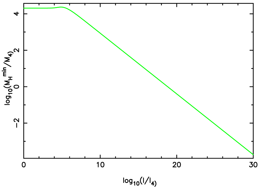
Figure 1: The minimum horizon mass after inflation as a function of the AdS radius. For $l/l_{4}\lesssim 10^{5}$ the constraint corresponds to inflation ending in the low-energy regime, whereas for larger $l$ it corresponds to the high-energy regime.

Consider a black hole formed from collapsing matter confined to the brane. It will have an event horizon that extends into the bulk. Moreover, if the size of the hole $r_{0}$ is much smaller than the AdS radius $l$ (and neglecting possible charges or rotation), it is natural to assume its geometry is given by a 5D Schwarzschild solution EHM99

$$ds_{5}^{2}=-f(r)\,dt^{2}+f^{-1}(r)\,dr^{2}+r^{2}\,d\Omega_{3}^{2}\,,$$ (22)

with $f(r)=1-r_{0}^{2}/r^{2}$ and $d\Omega_{3}$ the volume element of a 3-sphere. This form of the metric is a good approximation in the vicinity of the event horizon, which is the region needed to analyze the Hawking effect. The black hole is expected to emit Hawking radiation both into the brane and the bulk by exciting the brane or bulk degrees of freedom. In the present model, only gravitational radiation can propagate in the bulk. It is worth noting that near the horizon, the induced metric on the brane is given by

$$ds_{4}^{2}=-f(r)\,dt^{2}+f^{-1}(r)\,dr^{2}+r^{2}\,d\Omega_{2}^{2}\,,$$ (23)

which is not the usual $4$D Schwarzschild metric. Indeed, this metric has an effective negative energy–momentum tensor outside the horizon that will modify the gray-body factors of radiation by quantum fields confined to the brane EHM20 . However, the effective potentials in the field propagation equations bear similarity to those of the standard treatment. They also vanish when approaching the horizon, reducing the propagation equations to free wave equations. Since the brane is tuned to be flat, the derivation of the Hawking process on the brane will essentially be identical to the standard case. As for the bulk, Hawking radiation in AdS space has been discussed in Ref. Hemming , where it was shown to be similar to the asymptotically-flat case.

The expressions for radius, area and temperature of the black hole are given in terms of the AdS radius $l$ and the black hole mass $M$ as

$$r_{0} = \sqrt{\frac{8}{3\pi}}\frac{M^{1/2}}{M_{5}^{3/2}}=\sqrt{\frac{8}{3\pi}}\left(\frac{l}{l_{4}}\right)^{1/2}\left(\frac{M}{M_{4}}\right)^{1/2}l_{4}\,,\quad\quad$$ (24)

$$A_{5} = 2\pi^{2}r_{0}^{3}\,,$$ (25)

$$T_{{\rm BH}} = \frac{1}{2\pi r_{0}}\,,$$ (26)

and hold provided $r_{0}\ll l$. This is to be contrasted with the usual $4$D result

$$T_{{\rm BH}}(4{\rm D})=\frac{M_{4}^{2}}{8\pi M}\,.$$ (27)

To estimate the lifetime, consider the number of particles of a certain species $j$, emitted in $D$-dimensional spacetime by a black hole of temperature $T_{{\rm BH}}$, in a time interval $dt$ and with momentum in the interval $(\mathbf{k},\mathbf{k}+d\mathbf{k})$:

$$dN_{j}=\sigma_{j}(k)\;\frac{dt}{{\rm exp}(\omega/T_{{\rm BH}})\pm 1}\;\frac{d^{D-1}k}{(2\pi)^{D-1}}\,,$$ (28)

with $\omega^{2}=k^{2}+m^{2}$ and $m$ the mass of the particle. The upper and lower sign apply to fermions and bosons respectively. As regards the absorption/emission cross-sections $\sigma_{j}$, summation over all angular modes is understood. In general, they depend on the species and frequency and must be determined numerically Page . Due to the different metrics Eq. (23) and Eq. (22), accurate determination of the cross-sections is beyond the scope of this paper. However, in the high-frequency limit all cross-sections reduce to the same expression (see below). In the low-frequency limit, the cross-sections decrease with frequency, approaching a finite value for spin-$0$ or spin-$1/2$ particles, whereas they vanish with increasing powers of frequency for higher-spin particles. This means the total energy emitted in higher-spin particles is suppressed relative to particles of lowest spin. These features are expected to carry over to the brane context, while the numerical factors may change somewhat.

The rate of energy loss by $D$-dimensional evaporation is obtained from Eq. (28) as

$$\frac{dM}{dt}=-\;\sum_{j}\int\sigma_{j}(k)\;\frac{\omega}{{\rm exp}(\omega/T_{{\rm BH}})\pm 1}\;\frac{d^{D-1}k}{(2\pi)^{D-1}}\,.$$ (29)

In the high-frequency limit ($\omega\gg T_{BH}$) all cross-sections become identical, namely

$$\sigma\approx\frac{A_{\mathrm{eff},D}}{4}\equiv\frac{\Omega_{D-2}\;r_{\mathrm{eff},D}^{D-2}}{4}\,,$$ (30)

where $\Omega_{D-2}$ is the volume of a $(D-2)$-sphere and $r_{\mathrm{eff},D}$ an effective radius for black-body emission, defined as  EHM20 ; ref6

$$r_{{\rm eff},D}=\left(\frac{D-1}{2}\right)^{1/(D-3)}\left(\frac{D-1}{D-3}\right)^{1/2}r_{0}\,.$$ (31)

Adopting this approximation for all cross-sections reduces Eq. (29) to Stefan’s law:

$$\frac{dM}{dt}\approx-g_{D}\;\tilde{\sigma}_{D}\,A_{\mathrm{eff},D}\,T^{D},$$ (32)

with $g_{D}$ composed of bosonic and fermionic degrees of freedom as

$$g_{D}=g_{D,\mathrm{bos}}+\frac{2^{D-1}-1}{2^{D-1}}\,g_{D,\mathrm{ferm}}\,.$$ (33)

Further, $\tilde{\sigma}_{D}$ denotes the $D$-dimensional Stefan–Boltzmann constant, defined per degree of freedom:

$$\tilde{\sigma}_{D}=\frac{\Omega_{D-2}}{4\;(2\pi)^{D-1}}\;\Gamma(D)\,\zeta(D),$$ (34)

with $\zeta(D)$ the Riemann zeta function.

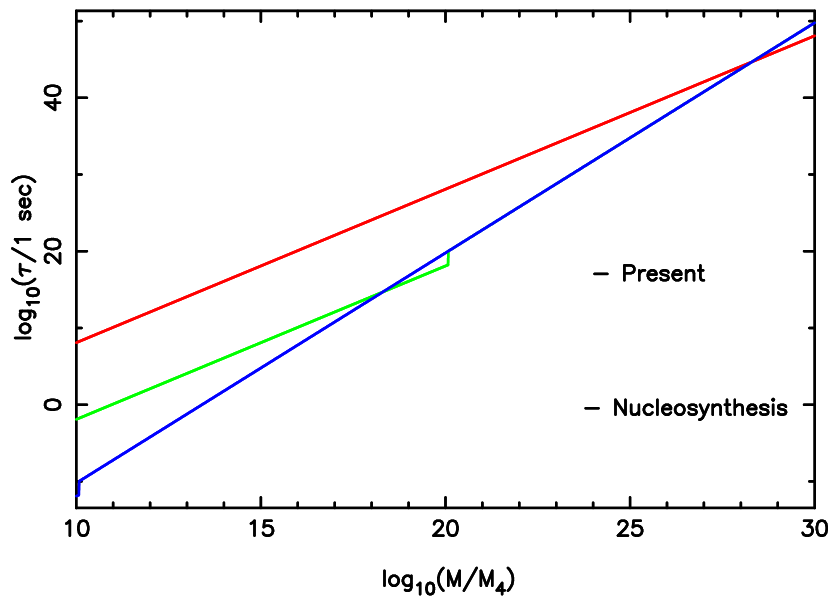
Figure 2: The lifetime of black holes of different initial masses, for the choices $l/l_{4}=10^{10}$, $10^{20}$ and $10^{30}$ (from bottom to top), approximating $\tilde{g}=0.032$ for all masses. For the lowest $l$ the usual 4D result applies across all the mass range, and for intermediate $l$ the discontinuity arises from the mismatch of the 4D and 5D relations across the transition. Lifetimes corresponding to nucleosynthesis and to the present age of the Universe are indicated.

In the present set-up, we thus estimate the total emitted power as

$$\frac{dM}{dt}\approx-g_{\mathrm{brane}}\tilde{\sigma}_{4}\tilde{A}_{\mathrm{eff},4}T^{4}-g_{\mathrm{bulk}}\tilde{\sigma}_{5}A_{\mathrm{eff},5}T^{5}\,,$$ (35)

where we must take $\tilde{A}_{\mathrm{eff},4}=4\pi r_{\mathrm{eff},5}^{2}$ because of the induced metric Eq. (23). Further, $g_{{\rm brane}}$ and $g_{{\rm bulk}}$ denote the brane and bulk degrees of freedom with rest masses lower than $T_{{\rm BH}}$. Since we have regarded $g_{{\rm bulk}}$ from the 5D point of view, it does not count the number of graviton Kaluza–Klein modes. Rather, it is the number of polarization states of the graviton, $D(D-3)/2$, which gives $g_{{\rm bulk}}=5$. The number of quantum fields into which the hole evaporates is approximately constant until its lifetime is nearly over. Then substituting the relevant expressions into Eq. (35) and integrating gives the lifetime $t_{{\rm evap}}$ of a black hole of initial mass $M$:

$$\frac{t_{{\rm evap}}(M)}{t_{4}}\approx\tilde{g}^{-1}\frac{l}{l_{4}}\,\left(\frac{M}{M_{4}}\right)^{2}\,,$$ (36)

with

$$\tilde{g}\equiv\frac{1}{160}\;g_{\mathrm{brane}}+\frac{9\zeta(5)}{32\pi^{4}}\;g_{\mathrm{bulk}}\,.$$ (37)

In the standard BH thermodynamics, Stefan’s law was shown to overestimate the emitted power Eq. (29) by a factor $2.6$ Page , and we therefore divide the first term of $\tilde{g}$ by the same factor, which should remain approximately true. The overestimate should be at least as severe for the bulk gravitational radiation, because of the higher spin suppression and the confining influence of the negative cosmological constant (although the latter supposedly would have little influence on small black holes); a more thorough analysis is required to be definite, but we divide by the same factor 2.6, resulting in a corrected form

$$\tilde{g}\approx 0.0024\;g_{{\rm brane}}+0.0012\;g_{{\rm bulk}}\,.$$ (38)

Since only gravity is allowed to propagate in the bulk, $g_{\rm bulk}$ simply counts the number of polarization states of the graviton, namely $D(D-3)/2=5$. Combined with the fact that $g_{{\rm brane}}>g_{{\rm bulk}}$, it is now apparent that evaporation into the bulk is a subdominant effect, even for very small black holes. We mention two typical values for $\tilde{g}$: If the black hole emits only massless particles we have $g_{\mathrm{brane}}=7.25$ and $\tilde{g}\approx 0.023$. If the hole is just hot enough to emit electron–positron pairs, we have $g_{\mathrm{brane}}=10.75$ and $\tilde{g}\approx 0.032$. Given the fairly qualitative nature of current observational constraints, results will be rather insensitive to the precise value of $\tilde{g}$.

By comparing with the lifetime of a black hole of same mass in standard relativity

$$\frac{t_{{\rm evap}}(M,4{\rm D})}{t_{4}}\approx 1.2\times 10^{4}\;g_{\mathrm{brane}}^{-1}\,\left(\frac{M}{M_{4}}\right)^{3}\,,$$ (39)

we find

$$\frac{t_{{\rm evap}}(M,5{\rm D})}{t_{{\rm evap}}(M,4{\rm D})}\sim\left(\frac{l}{r_{0}(5{\rm D})}\right)^{2}\,.$$ (40)

For a fixed mass, small black holes can have much longer lifetimes in the higher-dimensional case.

Figure 2 shows the lifetimes of black holes for three choices of the AdS radius. As will become clear in the following sections, for $l=10^{20}l_{4}$, corresponding to a brane tension $\lambda^{1/4}=10^{9}{\rm GeV}$, black holes initially of the AdS radius would be evaporating around the present epoch, and so this $l$ marks the transition between whether presently-evaporating black holes are effectively four or five dimensional. For values of $l$ higher than this, black holes evaporating today have lower initial masses than the usual $10^{20}\,M_{4}\simeq 10^{15}\,{\rm g}$.

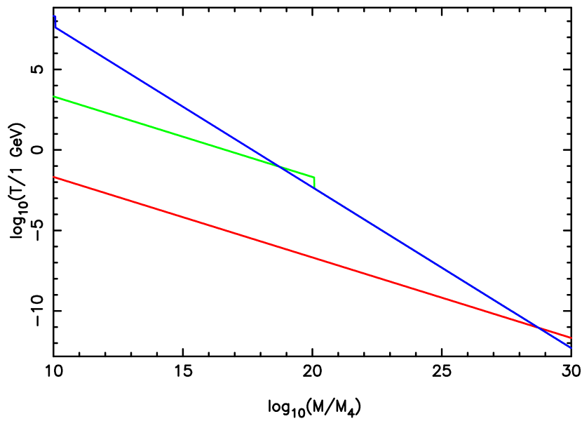
Figure 3: As Figure 2 but showing the initial temperature, with the top line corresponding to the lowest $l$.

Figure 3 shows the initial temperatures of black holes for the same choices of $l$. Most of the energy of a PBH is radiated at temperatures close to the initial temperature, with only a small fraction in a high-energy tail as the evaporation culminates. For $l\gtrsim 10^{20}l_{4}$, the temperature of black holes evaporating at the present is reduced.

For future reference, we list the $5\rm{D}$ expressions for mass and temperature in terms of the lifetime

$$\frac{M}{M_{4}} = \tilde{g}^{1/2}\left(\frac{t_{{\rm evap}}}{t_{4}}\right)^{1/2}\left(\frac{l}{l_{4}}\right)^{-1/2}\,,$$ (41)

$$\frac{T_{{\rm BH}}}{T_{4}} = \sqrt{\frac{3}{32\pi}}\;\tilde{g}^{-1/4}\left(\frac{t_{{\rm evap}}}{t_{4}}\right)^{-1/4}\left(\frac{l}{l_{4}}\right)^{-1/4}\,,$$ (42)

where $T_{4}=M_{4}$ is the 4D Planck temperature.

III.2 Ranges

The mass–lifetime relation Eq. (41) was derived under the assumption that the initially formed black hole is small, $r_{0}\ll l$. Using the mass–radius relation Eq. (24), this implies the consistency condition

$$\frac{M}{M_{4}}\ll\frac{l}{l_{4}}\,.$$ (43)

Thus, for a black hole of a given $\it{lifetime}$ there is an allowed range of values of $l$ for which it is small, obtained by substituting the mass–lifetime relation into condition Eq. (43):

$$l_{{\rm min}}\ll l\ll l_{{\rm max}}\,,$$ (44)

with

$$l_{{\rm min}}(t_{{\rm evap}})=\tilde{g}^{1/3}\left(\frac{t_{{\rm evap}}}{t_{4}}\right)^{1/3}\l_{4}\,,$$ (45)

and $l_{{\rm max}}$ the experimental upper limit on the AdS radius quoted earlier.

Using Eqs. (41) and (42), this corresponds to a range on the initial mass and temperature. The mass ranges from

$$M_{{\rm min}} \equiv M(t_{{\rm evap}},l_{{\rm max}})$$ (46)

$$= \left(\frac{l_{{\rm max}}}{l_{4}}\right)^{-1/2}\tilde{g}^{1/2}\left(\frac{t_{{\rm evap}}}{t_{4}}\right)^{1/2}M_{4}$$

to

$$M_{{\rm max}}\equiv M(t_{{\rm evap}},l_{{\rm min}})=\tilde{g}^{1/3}\left(\frac{t_{{\rm evap}}}{t_{4}}\right)^{1/3}\;M_{4}\,.$$ (47)

As for the black hole temperature, it ranges from

$$T_{{\rm BH,min}} \equiv T_{{\rm BH}}(t_{{\rm evap}},l_{{\rm max}})$$

$$= \sqrt{\frac{3}{32\pi}}\left(\frac{l_{{\rm max}}}{l_{4}}\right)^{-1/4}\tilde{g}^{-1/4}\left(\frac{t_{{\rm evap}}}{t_{4}}\right)^{-1/4}T_{4}$$

to

$$T_{{\rm BH,max}} \equiv T_{{\rm BH}}(t_{{\rm evap}},l_{{\rm min}})$$ (49)

$$= \sqrt{\frac{3}{32\pi}}\;\tilde{g}^{-1/3}\left(\frac{t_{{\rm evap}}}{t_{4}}\right)^{-1/3}T_{4}\,.$$

We note that, although the braneworld scenario allows PBHs of a given lifetime to be lighter than in the standard case, their initial temperature will be lower as well.

The maximum values are essentially what is obtained in the standard 4D theory, where $M\approx 0.04\;g_{\mathrm{brane}}^{1/3}\;(t_{{\rm evap}}/t_{4})^{1/3}\;M_{4}$ and $T_{{\rm BH}}\approx g_{\mathrm{brane}}^{-1/3}\;(t_{{\rm evap}}/t_{4})^{-1/3}\;T_{4}$. This should come as no surprise, since they correspond to the limit of what can be considered a small black hole. Well beyond that limit, i.e. for much smaller values of the AdS radius, the initial size (on the brane) of a black hole of the same lifetime would have been large, and it would have started out with properties indistinguishable from a $4$D black hole EHM99 . At a certain stage, the size of the hole will become comparable with the AdS radius, a transition stage that has so far eluded accurate description. But this happens near the end of its lifetime, when most of its mass has evaporated. For those black holes, we use the conventional estimates for the mass–lifetime relation etc.

Two examples are of particular interest in terms of observational consequences. The first concerns PBHs with lifetime equal to the present age of the universe. The currently-favoured low-density flat cosmology has an age of about 14 gigayears, i.e. $t_{0}\approx 8\times 10^{60}\;t_{4}$. The AdS radius marking the transition between 4D and 5D behaviour is $l_{{\rm min}}=7\times 10^{19}\,l_{4}$. The mass then ranges from $M_{{\rm max}}=4\times 10^{14}{\rm g}$ in the standard scenario, to $M_{{\rm min}}=3\times 10^{9}{\rm g}$ for $l=l_{{\rm max}}=10^{31}\;l_{4}$. The allowed temperatures range from $T_{{\rm BH,max}}=25\;\mathrm{MeV}$ in the standard scenario to $T_{{\rm BH,min}}=50\,\mathrm{keV}$ for $l=l_{{\rm max}}$. Note that 4D PBHs are hot enough to copiously emit electrons, whereas only massless Standard Model particles can be emitted for large values of the AdS radius.

As a second example, consider the era of nucleosynthesis ($t_{{\rm nuc}}\approx 100\,{\rm s}\approx 10^{44}\,t_{4}$). Taking $g_{{\rm brane}}=100$, we find $l_{{\rm min}}=10^{15}\,l_{4}$. The mass ranges from $M_{{\rm max}}=5\times 10^{9}{\rm g}$ in the standard scenario to $M_{{\rm min}}=2\times 10^{2}{\rm g}$ for $l=l_{{\rm max}}$. The temperatures range from $T_{{\rm BH,max}}=2\times 10^{3}\,\mathrm{GeV}$ to $T_{{\rm BH,min}}=0.2\,\mathrm{GeV}$.

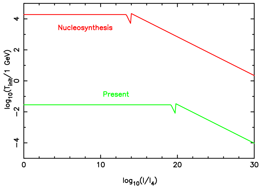
Figure 4: The initial temperature of black holes evaporating at the key epochs of nucleosynthesis and the present, shown as a function of $l$.

The initial temperatures of PBHs evaporating at these two epochs are shown as a function of $l$ in Figure 4.

IV Formation and Evolution

We now return to the cosmology of Section II. There are several mechanisms by which black holes could have formed in the early universe (see Ref. Carr85 for a review.) We focus on collapse of primordial density fluctuations.

IV.1 Formation mass

The end stage of the collapse process is highly nonlinear, and it is difficult to be very precise, as the formation masses remain poorly understood even in the standard cosmology. However it can be argued that the mass of the hole will be of order the Hubble horizon mass at the time of formation, $t_{i}$, by studying the Jeans mass. Consider a slightly overdense region of energy density $\tilde{\rho}$. Its density contrast is defined as $\delta=(\tilde{\rho}-\rho)/\tilde{\rho}$. Expanding the density contrast in Fourier modes, perturbation theory provides evolution equations for these modes, as long as $\delta\ll 1$. The Jeans length $L_{{\rm J}}$ is then defined such that modes with wavelength bigger than $L_{{\rm J}}$ are growing modes, while those with smaller wavelength oscillate. In Ref. ref10 the mode equations for the Friedmann model were given for a braneworld scenario. Applied to the present model, they read

$$\ddot{\delta}_{k}+H\;\dot{\delta}_{k}+\left[-\frac{16\pi}{3M_{4}^{2}}\;\rho-\frac{24\pi}{M_{4}^{2}}\;\frac{\rho^{2}}{\lambda}+\frac{1}{3}\left(\frac{k}{a}\right)^{2}\right]\delta_{k}=0\,.$$ (50)

Here, $k$ denotes the comoving wavenumber of the mode. The Jeans length is obtained by setting the expression in the brackets to zero. In the high-energy regime we can neglect the first term, leading to

$$L_{{\rm J}}=\frac{\pi}{3}\sqrt{\frac{2}{3}}R_{H}\approx 0.85\;R_{H}.$$ (51)

Just as in standard cosmology, in the high-energy regime the Jeans length is of order the horizon size.

The scenario for forming PBHs is the standard one. One starts with a slightly overdense region in a flat FRW Universe, on a scale much larger than the horizon. Because of the superhorizon scale, the region can separately be described as a portion of a closed FRW model Harrison ; Carr75 . Therefore, it will expand less rapidly than the environment, and the density contrast will grow. At a certain time the region will cross the Jeans scale. If the density contrast is still very small at that time, its evolution will be accurately described by Eq. (50), and it will start to oscillate, preventing collapse from ever occurring. Thus, a necessary condition for black hole collapse is $\delta\gtrsim 1$ at ‘Jeans’ crossing, which as shown above is more or less at horizon crossing.

To keep account of the uncertainty in the precise formation mass, we introduce a factor $f$ as follows:

$$M_{i}=f\;M_{H}(t_{i})\,.$$ (52)

A certain amount of controversy exists over the possible range of $f$, although, recent numerical studies seem to favour $f\sim 1$ NJ . Moreover, we find in general that the constraints examined in the companion paper will turn out not to be too sensitive to its exact value.

IV.2 Formation time

First consider PBHs forming in the high-energy regime. Then by assumption it holds that $t_{i}\ll t_{c}$. By substituting the expressions (12) and (9) for horizon radius and transition time, this translates into

$$R_{H}(t_{i})\ll 2\,l\,.$$ (53)

Since the mass of the PBH is not expected to be larger than the horizon mass, its initial radius will not be larger than the horizon. It is clear from Eq. (53) that PBHs formed in the high-energy regime are $\it{small}$ and effectively 5-dimensional. The formation time can be expressed in terms of the initial mass or lifetime, by substituting Eqs. (12) and (9) into Eq. (52) and using the mass–lifetime relation Eq. (41):

$$\frac{t_{i}}{t_{4}} = \frac{1}{4}f^{-1/2}\left(\frac{M_{i}}{M_{4}}\right)^{1/2}\left(\frac{l}{l_{4}}\right)^{1/2}$$ (54)

$$= \frac{1}{4}f^{-1/2}\tilde{g}^{1/4}\left(\frac{t_{{\rm evap}}}{t_{4}}\right)^{1/4}\left(\frac{l}{l_{4}}\right)^{1/4}\,.$$

In the standard regime, the formation time is given through Eq. (15) as

$$\frac{t_{i}}{t_{4}}=f^{-1}\frac{M_{i}}{M_{4}}=0.04\;f^{-1}g_{\mathrm{brane}}^{1/3}\left(\frac{t_{{\rm evap}}}{t_{4}}\right)^{1/3}\,,$$ (55)

which now must satisfy $t_{i}\gg t_{c}$. Thus $f^{-1}M/M_{4}\gg 0.5\;l/l_{4}$, which violates condition Eq. (43). As could be expected, a black hole formed in the standard regime will be large, and behaves for the vast majority of its lifetime as a 4D object.

Using Eqs. (24) and (12) it is straightforward to show that

$$r_{0}=f^{1/2}\sqrt{\frac{8}{3\pi}}4t_{i}\approx f^{1/2}R_{H},$$ (56)

i.e. that at the formation time, $t_{i}$, the Schwarzschild radius associated with the collapsing perturbation, of mass $M_{i}$, is of order the horizon size, $R_{H}$, so long as $f$ is not much smaller than 1. This is important since it implies that the collapsing perturbation will fall within its Schwarzschild radius and so form a black hole very soon after entering the horizon. Hence, as with the standard PBH scenario it is reasonable to assume that we need not concern ourselves too greatly with details such as the anisotropy and inhomegeneity of the collapse in the nonlinear subhorizon regime, since the black hole should form before any such effects have a chance to act.

Finally, we note that the minimum mass enforced by the condition that PBHs form after inflation guarantees that their mass will be much greater than the Planck mass relevant at that time (either $M_{5}$ in the high-energy regime or $M_{4}$ in the low-energy regime), which in turn means that their lifetime will be much greater than the formation time.

IV.3 Evolution

Once the black holes have formed, their evolution must be followed forwards in time to the epoch where observational constraints might apply, either the present epoch or the time of evaporation. As the PBH comoving number density is constant up until evaporation, as usual the relative density of PBHs as compared to radiation will grow proportional to the scale factor while evaporation is negligible. A common approximation is to presume that evaporation is negligible right up until the lifetime of the PBH is reached, at which point its entire mass–energy is released with products characteristic of its initial temperature, and this approximation continues to be good in the braneworld case.

V Conclusions

We have carried out a detailed investigation of how primordial black hole scenarios are modified in the RS-II braneworld. Whether these changes are significant depends on the AdS radius $l$ of the braneworld model; if this is sufficiently small then the standard scenario is recovered. However, current constraints on the AdS radius are very weak ($l\lesssim 10^{31}\,l_{4}$ where $l_{4}$ is the 4-dimensional Planck length), and substantial modifications to the usual case are possible for black holes evaporating at any epoch. If the AdS radius exceeds $10^{15}\,l_{4}$ then the properties of PBHs evaporating at nucleosynthesis (or earlier) are modified, and if it exceeds $10^{20}l_{4}$ PBHs evaporating up to the present epoch are affected. PBHs will have modified evolution if and only if they form during the high-energy phase of braneworld cosmological evolution.

If braneworld effects are important, they act to reduce the mass of a black hole surviving to a given epoch. More importantly, they give a reduced temperature, which will alter the evaporation products characteristic of such PBHs. An important application of these results is to investigate how constraints on PBH abundances are modified in the braneworld scenario. Because the black holes surviving to key epochs such as nucleosynthesis and the present can have modified temperatures, the standard astrophysical constraints cannot be applied and must be rederived from scratch. We carry out this analysis in a forthcoming companion paper (Clancy et al.).

Throughout we have ignored the possibility that PBHs might grow significantly through accretion of the background, known to be a valid approximation in the standard cosmology Carr75 . However in the high-energy regime this issue deserves re-investigation, which we will do in a forthcoming paper.

We have considered the simplest of braneworlds. It would be interesting to see how robust our conclusions are in more complicated cosmological models, for instance those including one or more bulk fields. Unless their number is very large, this will not drastically alter the energy fraction a black hole loses to the brane as compared to the bulk. On the other hand, the early phase of 4D cosmology can be significantly modified, in turn altering the relation between the black hole’s lifetime and time of formation. This is left for future investigation.

- (1) Ya. B. Zel’dovich and I. D. Novikov, Astron. Zh. 43, 758 (1966) [Sov. Astron. 10, 602 (1967)]; S. W. Hawking, Mon. Not. Roy. Ast. Soc. 152, 75 (1971); B. J. Carr and S. W. Hawking, Mon. Not. Roy. Ast. Soc. 168, 399 (1974).
- (2) S. W. Hawking, Commun. Math. Phys. 43, 199 (1975); I. D. Novikov, A. G. Polnarev, A. A. Starobinsky, and Ya. B. Zel’dovich, Astron. Astrophys. 80, 104 (1979); M. Yu. Khlopov and A. G. Polnarev, Phys. Lett. B97, 383 (1980); B. J. Carr and J. E. Lidsey, Phys. Rev. D48, 543 (1993); B. J. Carr, J. H. Gilbert, and J. E. Lidsey, Phys. Rev. D50, 4853 (1994), astro-ph/9405027; A. M. Green and A. R. Liddle, Phys. Rev. D56, 6166 (1997), astro-ph/9704251.
- (3) B. J. Carr, Astrophys. J. 201, 1 (1975).
- (4) B. J. Carr, Observational and Theoretical Aspects of Relativistic Astrophysics and Cosmology edited by J. L. Sanz and L. J. Goicoechea (World Scientific, Singapore, 1985).
- (5) P. Argyres, S. Dimopoulos, and J. March-Russell, Phys. Lett. B441, 96 (1998), hep-th/9808138.
- (6) R. Casadio and B. Harms, Phys. Rev. D 64, 024016 (2001), hep-th/0101154; P. Kanti and J. March-Russell, hep-ph/0203223.
- (7) R. Emparan, G. T. Horowitz, and R. C. Myers, Phys. Rev. Lett. 85, 499 (2000), hep-th/0003118.
- (8) L. Randall and R. Sundrum, Phys. Rev. Lett. 83, 4690 (1999), hep-th/9906064.
- (9) C. Csaki, M. Graesser, C. Kolda, and J. Terning, Phys. Lett. B462, 34 (1999), hep-ph/9906513; J. M. Cline, C. Grojean, and G. Servant, Phys. Rev. Lett. 83, 4245 (1999), hep-ph/9906523; P. Binétruy, C. Deffayet, U. Ellwanger, and D. Langlois, Phys. Lett. B477, 285 (2000), hep-th/9910076; T. Shiromizu, K. I. Maeda, and M. Sasaki, Phys. Rev. D62, 024012 (2000), gr-qc/9910076; R. Maartens, Phys. Rev. D62, 084023 (2000), hep-th/0004166; R. Maartens, gr-qc/0101059.
- (10) C. D. Hoyle, U. Schmidt, B. R. Heckel, E. G. Adelberger, J. H. Gundlach, D. J. Kapner, and H. E. Swanson, Phys. Rev. Lett. 86, 1418 (2001), hep-ph/0011014.
- (11) P. Binétruy, C. Deffayet, U. Ellwanger, and D. Langlois, Phys. Lett. B477, 285 (2000), hep-th/9910076; J. D. Barrow and R. Maartens, gr-qc/0108073.
- (12) D. Langlois, R. Maartens, and D. Wands, Phys. Lett. B489, 259 (2000).
- (13) A. R. Liddle and D. H. Lyth, Cosmological Inflation and Large-Scale Structure, Cambridge University Press, Cambridge, 2000.
- (14) N. Dadhich and S. G. Ghosh, Phys. Lett. B518, 1 (2001) hep-th/0101019.
- (15) M. Bruni, C. Germani, and R. Maartens, Phys. Rev. Lett. 87, 231302 (2001) gr-qc/0108013.
- (16) N. Dadhich, R. Maartens, P. Papadopoulos, and V. Rezania, Phys. Lett. B487, 1 (2000), hep-th/0003061.
- (17) K. S. Thorne in Magic without magic: John Archibald Wheeler, J. Klauder, ed. (Freeman, 1972).
- (18) K. Nakao, K. Nakamura, and T. Mishima, gr-qc/0112067.
- (19) R. Emparan, G. T. Horowitz, and R. C. Myers, JHEP 0001, 007 (2000), hep-th/9911043.
- (20) S. Hemming and E. Keski-Vakkuri, Phys. Rev. D64, 044006 (2001), gr-qc/0005115.
- (21) D. N. Page, Phys. Rev. D13, 198 (1976).
- (22) N. Sanchez, Phys. Rev. D18, 1030 (1978).
- (23) P. Brax, C. van de Bruck, and A. C. Davis, JHEP 0110, 026 (2001), hep-th/0108215.
- (24) E. R. Harrison, Phys. Rev. D1, 2726 (1970).
- (25) J. C. Niemeyer and K. Jedamzik, Phys. Rev. D59, 124013 (1999), astro-ph/9901292.