STELLAR-MASS BLACK HOLES
IN THE SOLAR NEIGHBORHOOD

Abstract

We search for nearby, isolated, accreting, “stellar-mass” ($3$ to $100M_{\odot}$) black holes. Models suggest a synchrotron spectrum in visible wavelengths and some emission in X-ray wavelengths. Of 3.7 million objects in the Sloan Digital Sky Survey Early Data Release, about 150,000 objects have colors and properties consistent with such a spectrum, and 87 of these objects are X-ray sources from the ROSAT All Sky Survey. Thirty-two of these have been confirmed not to be black-holes using optical spectra. We give the positions and colors of these 55 black-hole candidates, and quantitatively rank them on their likelihood to be black holes. We discuss uncertainties the expected number of sources, and the contribution of black holes to local dark matter.

1 INTRODUCTION

Since they were first postulated, black holes have captured the imagination of scientists, as well as the general public. In addition to their intrinsic appeal, black holes potentially impact on a number of fundamental problems in physics and astronomy. They are a possible endpoint of stellar evolution. They provide a unique laboratory in which to study strong gravity. Knowledge of the mass and spatial distributions of black holes could also provide information about stellar evolution, galaxy formation, and dark matter.

While they are among the most interesting astrophysical objects, black holes, by their very nature (“black”), are difficult to isolate and study. Since the intrinsic Hawking radiation from black holes of the mass we study (greater than about a solar mass) is quite feeble, the search for black holes must concentrate on the interaction of the black hole with the surrounding medium. Thus, the search strategy for black holes depends upon the hole mass.

We can organize black holes in groups according to their mass. Super-massive black holes with mass of order $10^{8}\,M_{\odot}$, are thought to reside in the nuclei of galaxies [for a review, see Kormendy & Richstone (1995)]. In addition to their role in the dynamics of galaxies and galaxy formation, they are believed to be the central engines of energetic phenomenon associated with active galactic nuclei.

Evidence for intermediate-mass black holes of around $10^{2}$ to $10^{5}\,M_{\odot}$ has recently been found (Matsumoto & Tsuru, 1999; Ptak & Griffith, 1999; Matsumoto et al., 2001; Kaaret et al., 2001). Intermediate-mass black holes might be precursors to super-massive black holes (Ebisuzaki et al., 2001).

Lower mass black holes formed at the endpoint of stellar evolution are known as remnant black holes (RBH). They are expected to have masses from about $3$ to $100M_{\odot}$, and are the focus of this paper. These remnant black holes are sometimes referred to as “stellar-mass” black holes. The lower mass limit derives from the upper mass limit of neutron stars, the other possible outcome for the core of a supernova. The upper mass is limited by the mass of the progenitor star and possible subsequent accretion onto the RBH. Remnant black holes in binary systems were first discovered through X-ray emission [see, e.g., Tanaka & Lewin (1996)]. The first observational hint for the existence of an isolated RBH comes from gravitational microlensing (Bennett et al., 2002; Mao et al., 2002).

A last group of black holes, which would have masses less than $3M_{\odot}$, could not have been formed through stellar evolution, but might have formed at an earlier time in the universe, presumably as primordial black holes.

Of the four groups, there is good evidence for the existence of the first three types of black holes. This paper discusses a search for candidates for isolated remnant black holes.

As mentioned, since black holes will not themselves be luminous, the key to detecting them is to observe their effect on their surroundings. Black holes will accrete and radiate some fraction of the accreting mass into energy. [For a review of black-hole accretion, see Chakrabarti (1996).]

For those RBHs that are part of a binary system, accretion is typically from the companion star through Roche lobe overflow onto an accretion disk. These objects were first discovered through their X-ray emission (Tanaka & Lewin, 1996), though detections have been made from radio to $\gamma$-ray frequencies. The accretion emission in the optical and near-infrared is dominated by that of the companion star.

For isolated RBHs, the subject of this study, the accretion is from the interstellar medium. The accretion rate from the ISM is typically much less than that from a companion star, so the corresponding luminosity of an isolated RBH is so small that they have yet to be detected. Since nearly half of all stars are in binary systems, we might expect the RBHs formed to have this same ratio. Thus, isolated RBHs should outnumber binary RBHs by 2:1.

Accretion emission is not the only proposed method for detecting RBHs. There is recent evidence (Bennett et al., 2002; Mao et al., 2002) for the detection of black holes using gravitational microlensing. Another method is looking for the effect of black hole creation in supernova light curves (Balberg & Shapiro, 2001). Finally, another method for finding a RBH is to look for the cutoff of neutrino emission due to black hole formation during a supernova (Beacom, Boyd & Mezzacappa, 2001).

The purpose of this paper is to identify a small number of isolated, nearby, RBH candidates for follow-up optical and X-ray studies. Our approach, following the suggestion of Heckler & Kolb (1996), is to search for objects in the Early Data Release (Stoughton et al., 2002) of the Sloan Digital Sky Survey (SDSS) (York et al., 2000) that are consistent with the type of power-law spectra expected from isolated RBHs. We also require that the source appear as an X-ray source in the ROSAT all-sky survey (Voges et al., 1999).

Heckler & Kolb (1996) suggested using the SDSS spectroscopic survey to detect RBHs. The photometric survey however is four to five magnitudes fainter so is sensitive to objects ten times further away, and will have a thousand times more objects than the spectroscopic survey. A possible disadvantage of the SDSS photometric survey is that it lacks detailed spectral information, making it more difficult to identify positively RBH candidates while simultaneously rejecting spurious stars. However, we find that the five color bands of the SDSS photometric survey are quite adequate for synthesizing the optical spectrum, and the cross-correlation with ROSAT eliminates the vast majority of stars.

In the following section we discuss theoretical issues and uncertainties involving the expected spectrum, the expected RBH mass and velocity distributions, and estimates of the number densities of RBHs.

In §3 we describe the search strategy, and §4 contains our results. We conclude in §5. The major result are tables of positions and color magnitudes of the RBH candidates.

2 THE SPECTRAL ENERGY DISTRIBUTION FOR ISOLATED REMNANT BLACK HOLES

In this section we discuss possible spectral energy distributions for isolated remnant black holes. The spectrum depends upon the mass of the hole and the local environment of the RBH (the density of the interstellar medium (ISM), and the velocity of the hole with respect to the ISM). Even with knowledge of the local conditions surrounding the RBH, there is still a great deal of uncertainty in the spectral energy distribution.

We can roughly classify RBH accretion models by geometry (spherical or disk-like) and type (thermal, advection-dominated, convection-dominated, etc). Most, if not all, accretion models utilize magnetic fields in one way or another. In all models, it is the resulting electron synchrotron radiation that dominates the spectrum in the optical region.

The first calculation of the spectrum of a black hole spherically accreting in the ISM was by Shvartsman (1971), and investigated by numerous authors [some early work includes Zeldovich & Novikov (1971); Novikov & Thorne (1973); Shapiro (1973)].

The estimates for observing black holes in Heckler & Kolb (1996) used a spherical accretion model and computed the spectrum using the method of Ipser & Price (1982) (hereafter, IP). The problem of spherical accretion was first solved by Bondi (1952), and the resulting accretion flow is termed a Bondi flow. Spectra have been computed for such flows by Ipser & Price (1982) and McDowell (1985). The basic result is that interstellar magnetic fields are drawn in and compressed in the accretion process, reaching about 10 tesla at the horizon for standard ISM conditions. The resulting synchrotron radiation can be quite high. The spectral energy distribution in such a model is indicated in Fig. 1 for a $10M_{\odot}$ RBH. The characteristic spectrum is a power-law (albeit with different power laws indices above and below the synchrotron peak).

Recently, Igumenshchev & Narayan (2002) have shown that spherical accretion may not be as simple as previous studies would indicate, due to the fact that the dynamical effects of magnetic fields on the accretion flow have not properly been taken into account. They perform three-dimensional magnetohydrodynamic simulations of an initially spherically symmetric system (assuming an initially uniform magnetic field), and show that the resulting flow is convectively unstable. This convective flow (which they term a convection-dominated Bondi flow, or CDBF) has a drastically decreased accretion rate compared to a Bondi flow (approximately 9 orders of magnitude for an RBH), which would drastically affect the emission spectrum. At this time there are no calculations of emission spectra from CDBFs in the literature. However, there are enough similarities between CDBF and CDAF models (discussed below) that one could use computed CDAF spectra (Ball, Narayan & Quataert, 2001) for CDBF spectra.

Even without the instability of Bondi flow, if there is sufficient inhomogeneity in the ISM due to density or velocity gradients, the accreting matter will have appreciable angular momentum and can form a disk (Fryxell & Taam, 1988; Taam & Fryxell, 1989). These inhomogeneities can also lead to disk reversal. Disk accretion has been extensively studied for X-ray binaries where it is believed that an accretion disk powers the X-ray emission. There, the disk forms when the accreting gas has non-zero angular momentum as it falls onto the compact object, such as through a solar wind or through Roche lobe overflow. The hydrodynamics of such a flow was first solved by Shakura & Sunyaev (1973). Since then, there have been a number of advancements in the field. In particular, for systems with low accretion rates (as expected for RBHs), one might expect the formation of an optically thin accretion disk.

The instabilities and inhomogeneities that lead to disk reversal also lead to variabilities on the same timescales mentioned in Heckler & Kolb (1996), equation 2 (reprinted here);

$$\Delta t\approx 10\left(\frac{M}{M_{\odot}}\right)\left(\frac{v}{10\ \textrm{km s}^{-1}}\right)^{-3}\ \textrm{yr}.$$ (1)

The advection-dominated accretion flow (ADAF) model (Ichimaru, 1977; Rees, Begelman & Phinney, 1982; Narayan & Yi, 1994; Abramowicz et al., 1995) has a two-temperature structure that results in a broadband spectra from radio to gamma rays. Fujita at al. (1998) compute spectra for a RBH using an ADAF model following the prescription of Manmoto, Mineshige & Kusunose (1997). A typical ADAF spectral energy distribution is also shown in Fig. 1. Like the IP spectrum, the spectrum around optical frequencies is a power-law synchrotron spectrum. Unlike the IP spectrum, there is appreciable luminosity at higher frequencies.

ADAF models are expected to be convectively unstable (Narayan & Yi, 1994; Begelman & Meier, 1982), and lead naturally to convection-dominated accretion flow (CDAF) models. In fact, Abramowicz & Igumenshchev (2001) have argued that recent Chandra observations of black hole and neutron star systems support CDAF, instead of ADAF, models. A typical CDAF spectral energy distribution is also shown in Fig. 1. Superficially it resembles the ADAF and IP spectra at optical frequencies (a power-law synchrotron spectrum with the peak possible in the optical region). Like ADAF models it has a high-energy peak; in fact the ratio of X-ray and $\gamma$-ray luminosity to synchrotron luminosity is even larger in the CDAF models than in ADAF models.

Clearly, the expected spectral energy distribution of accreting RBHs is a complicated problem and it is impossible to specify the spectrum with complete confidence. Nevertheless, for our purposes we can make the general assumption that for optical frequencies the spectrum is synchrotron, possibly with the peak frequency, $\nu_{\textrm{peak}}$, in the optical region. The location of the synchrotron peak scales with the mass of the black hole; using the ADAF model of Manmoto, Mineshige & Kusunose (1997), $\nu_{\textrm{peak}}\propto M^{-3/8}$. The result is a broken power-law spectrum, possibly making the transition in the visible region of the electromagnetic spectrum from a positive slope for $\nu<\nu_{\textrm{peak}}$ to a constant negative slope for $\nu>\nu_{\textrm{peak}}$. We also assume that there is an appreciable X-ray luminosity.

In addition to the accretion luminosity, it was shown in Armitage & Natarajan (1999) that there could be a substantial (equaling or exceeding the accretion luminosity) energy emission due to the Blandford-Znajek effect (Blandford & Znajek, 1977) if the black hole is rotating. This energy is likely emitted at $\gamma$-ray frequencies, so we do not consider this model here.

3 ESTIMATE OF THE NUMBER OF EXPECTED SOURCES

There are a number of uncertain parameters that enter into the estimate of the expected number of detected sources. The parameters can be broadly grouped under the following categories: (i) There are parameters that describe the properties of the ISM. The properties of the ISM determine the accretion rate, and hence the total luminosity of an object. (ii) There are parameters that specify the number density of black holes as a function of their mass and the distribution of hole velocities with respect to the ISM. The luminosity, as well as the spectrum (in particular, $\nu_{\textrm{peak}}$) depends upon the mass of the hole. Naturally, the number of detected sources will scale with the normalization of the RBH mass distribution function, i.e., the overall density of black holes. The accretion rate depends upon the velocity of the hole. (iii) The emission model (IP, ADAF, CDAF, etc.) determines the spectrum of the holes. Because of the complexity of the emission models we must parameterize the model spectra. (iv) Finally, observational parameters such as spectral coverage and limiting magnitude determine the number of expected source detections.

The total luminosity of the RBH will depend on the accretion rate. The RBH accretion rate is a sensitive function of the black hole mass and velocity with respect to the ISM: for an object of mass $M$ moving supersonically with velocity $v$, $\dot{M}\propto M^{2}v^{-3}$ (for fixed ISM conditions). Thus, in order to make predictions or place upper limits on RBH density, it is important to consider an appropriate model for the RBH mass function and velocity distribution.

A natural method of determining the RBH mass function and velocity distribution would be to start from an underlying progenitor star population and use that to infer the RBH properties. Thus, in this work we assume a power law mass function and Maxwellian velocity distribution, as follows. Let $\Phi(M,v)dMdv$ be the number of RBH’s per cubic parsec in the range $(M,M+dM)$, $(v,v+dv)$, and assume $\Phi(M,v)$ factorizes as

$$\Phi(M,v)=\phi_{M}(M)\phi_{v}(v),$$ (2)

where

$$\phi_{M}(M)=\phi_{0}\left(\frac{M}{M_{\odot}}\right)^{-(1+x)}$$ (3)

and

$$\phi_{v}(v)=\left(\frac{2}{\pi}\right)^{1/2}\frac{v^{2}}{\sigma^{3}}\exp\left(-\frac{v^{2}}{2\sigma^{2}}\right).$$ (4)

Here, $x$ determines the power law slope of the mass function and $\sigma$ is the velocity dispersion. Fryer & Kalogera (2001) have derived the theoretical RBH mass function starting from a power law progenitor mass function, and their results suggest the slope of the power law does not change when a star becomes a RBH. On the assumption that the RBH mass distribution is not much different from the stellar mass distribution from which it is formed, we take $x=2$. We assume the RBHs range in mass from 3 to 100 $M_{\odot}$.

We will assume that the velocity dispersion of the RBH’s is similar to that of the X-ray-binary population, $\sigma=40\ \textrm{km s}^{-1}$ (Hansen & Phinney, 1997; White & van Paradjis, 1996; van Paradjis & White, 1995).

The ISM parameters that enter are the sound speed ($c_{s}$) and the mass density ($\rho_{\infty}$) of the ISM. The relevant black hole distribution parameters are the local mass density of black holes ($\rho_{BH}$), the velocity dispersion of the black holes ($\sigma$), the slope of the black-hole mass function ($x$), and the maximum and minimum black hole masses ($M_{min},M_{max}$). The emission model parameters include an overall factor describing the efficiency of conversion of accreting mass to luminosity in each bandpass (the five SDSS bands $u^{*},\ g^{*},\ r^{*},\ i^{*},\ z^{*}$, X-ray, IR, etc.): $\epsilon_{\alpha}\equiv L_{\alpha}/\dot{M}$ where $L_{\alpha}$ is the luminosity in band $\alpha$ and $\dot{M}$ is the accretion rate. Note that all the model dependence (CDAF, IP, etc.) is hidden in the efficiencies $\epsilon_{\alpha}$. Finally, the observational parameters include the solid angle of sky covered ($\Omega_{SDSS}$) and the minimum detectable flux in each bandpass ($F^{min}_{\alpha})$.

Fryer & Kalogera (2001) suggests that black holes receive a “kick” when formed, similar to what happens when neutron stars formed, on the order of 100 km s^-1. Popov & Prokhorov (1998) have modeled the spatial distribution of accretion luminosity from isolated accreting RBHs and neutron stars in our galaxy. They show the luminosity has a toroidal structure (centered and in the plane of the galaxy) with radius of about 5 to 6 kpc for neutron stars, and about 4 to 8 kpc for black holes. They additionally incorporate the effect of supernova kicks, using characteristic values of 200 km s^-1 and 400 km s^-1.

The SN kick can have a profound effect on the velocity distribution, depending on the values of the kick velocity $k$ and velocity dispersion $\sigma$. As an example, consider an initial stellar population (all of which will evolve to SN and become RBHs) with a Maxwellian velocity distribution. We then randomly “kick” every object in this population. Averaging over the kick direction, we obtain

$$\phi_{\textrm{kicked}}(v)=\left(\frac{2}{\pi}\right)^{1/2}\frac{v^{2}}{\sigma^{3}}\left[\left(1+\frac{k^{2}}{v^{2}}\right)I_{0}\left(-\frac{vk}{\sigma^{2}}\right)+2\frac{k}{v}I_{1}\left(-\frac{vk}{\sigma^{2}}\right)\right]\exp\left[-\frac{v^{2}+k^{2}}{2\sigma^{2}}\right],$$ (5)

where $I_{0}(x)$ and $I_{1}(x)$ are modified Bessel functions. Whereas a purely Maxwellian velocity distribution has very few members near $v=0$ ($\phi_{v}(0)=0$), a kicked Maxwellian velocity distribution can have a significant amount:

$$\phi_{\textrm{kicked}}(0)=\left(\frac{2}{\pi}\right)^{1/2}\frac{k^{2}}{\sigma^{3}}\exp\left(-\frac{k^{2}}{2\sigma^{2}}\right).$$ (6)

The “low-velocity” population will have a larger accretion rate, and lead to more sources than in our “unkicked” model.

Now we turn to the estimate of $N_{\alpha}$, the number of RBH’s observable in the SDSS survey in each bandpass. We start with

$$dN_{\alpha}=\frac{\Omega_{SDSS}}{3}\ d_{\alpha-max}^{3}(M,v)\ \Phi(M,v)\ dMdv,$$ (7)

where $\Omega_{SDSS}$ is the solid angle of the SDSS, $\Phi(M,v)$ is the distribution function from the previous section, and $d_{\alpha-max}$ is defined for each bandpass as the effective maximum distance to a detectable source:

$$L_{\alpha}=4\pi F^{min}_{\alpha}d_{\alpha-max}^{2}=\epsilon_{\alpha}\dot{M}.$$ (8)

Since we parameterize the luminosity in each bandpass by a single parameter $\epsilon_{\alpha}$, we must calculate $\dot{M}$. The accretion rate is well approximated by (Bondi, 1952):

$$\dot{M}=\pi r_{A}^{2}\rho_{\infty}\sqrt{v^{2}+c_{s}^{2}}$$ (9)

where the accretion radius is defined as

$$r_{A}=\frac{2GM}{v^{2}+c_{s}^{2}},$$ (10)

with $v$ the velocity, and $c_{s}$ the sound speed. Let $\beta_{s}\equiv v/c_{s}$. Then

$$\dot{M}=\frac{4\pi G^{2}M_{\odot}^{2}\rho_{\infty}}{c_{s}^{3}}\left(\frac{M}{M_{\odot}}\right)^{2}\left(1+\beta_{s}^{2}\right)^{-3/2}.$$ (11)

Solving for $d_{\alpha-max}$ from its definition in equation (8), and using equation (11) for $\dot{M}$, we obtain

$$d_{\alpha-max}=\left(\frac{L_{\alpha}}{4\pi F^{min}_{\alpha}}\right)^{1/2}=(GM_{\odot})\epsilon_{\alpha}^{1/2}\rho_{\infty}^{1/2}\left(F^{min}_{\alpha}\right)^{-1/2}c_{s}^{-3/2}\left(\frac{M}{M_{\odot}}\right)(1+\beta_{s}^{2})^{-3/4}.$$ (12)

In general, one expects $\epsilon_{\alpha}$ to be a function of $M$, $\dot{M}$, $v$, etc. There are not a lot of calculations of model spectral energy densities for the mass range and accretion rates of interest to us. Of the relevant calculations that do exist, there are more ADAF calculations than CDAF calculations. So in estimating $\epsilon_{\alpha}$ we will be guided by the ADAF calculations. Manmoto, Mineshige & Kusunose (1997) have studied the features of ADAF spectra. Their results are consistent with most of the energy in the optical region in a broken-power-law spectrum. They find the peak frequency to scale as

$$\nu_{\textrm{peak}}(M)=10^{15}\left(\frac{M_{\odot}}{M}\right)^{3/8}\ \textrm{Hz}.$$ (13)

They also find that the peak value of the spectral energy distribution to be

$$\left[\nu L_{\nu}\right]_{\textrm{peak}}=3\times 10^{-3}\dot{M},$$ (14)

independent of the mass of the hole. The value of $\left[\nu L_{\nu}\right]_{\textrm{peak}}$ is roughly the total integrated luminosity.

It is convenient to express $\epsilon_{\alpha}$ as a product of the total fraction of $\dot{M}$ that is radiated (integrated over all frequencies), times the fraction radiated in band $\alpha$:

$$\epsilon_{\alpha}=\epsilon\times f_{\alpha}=2\times 10^{-3}\left(\frac{\epsilon}{2\times 10^{-3}}\right)\ f_{\alpha}.$$ (15)

The definition of $f_{\alpha}$ is

$$f_{\alpha}=\frac{\int_{\alpha}\left[\nu L_{\nu}\right]\left(d\nu/\nu\right)}{\int_{0}^{\infty}\left[\nu L_{\nu}\right]\left(d\nu/\nu\right)},$$ (16)

where the “alpha” notation in the numerator implies integration over the range of frequencies appropriate for band $\alpha$. The frequencies for the various SDSS filters are given in Table 1 and Fig. 2.

To estimate $f_{\alpha}$, assume the simple broken-power-law spectrum for $\left[\nu L_{\nu}\right]$

$$\left[\nu L_{\nu}\right]=\left[\nu L_{\nu}\right]_{\textrm{peak}}\left\{\begin{array}[]{ll}(\nu/\nu_{\textrm{peak}})^{3}&(\nu<\nu_{\textrm{peak}})\\ (\nu/\nu_{\textrm{peak}})^{-2}&(\nu>\nu_{\textrm{peak}}).\\ \end{array}\right.$$ (17)

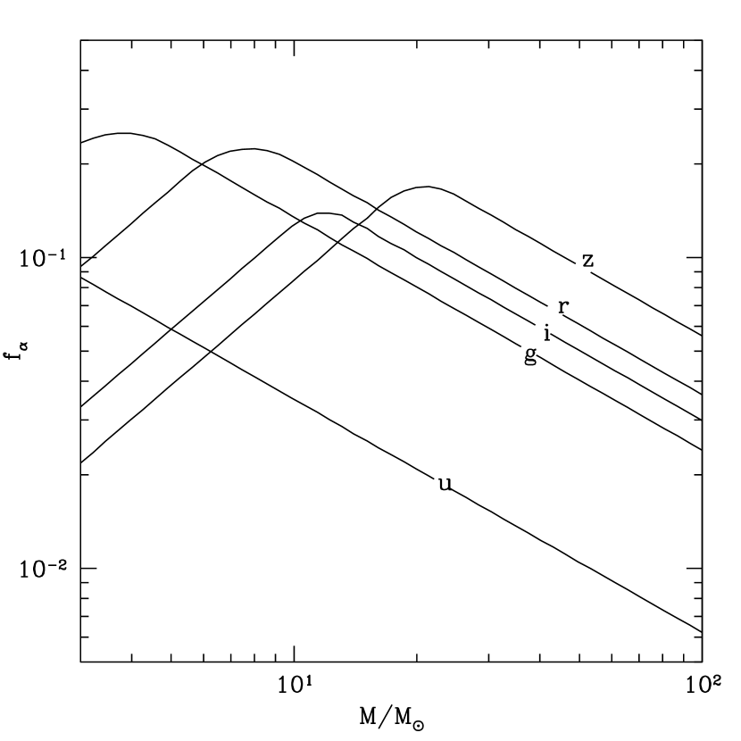
Figure 3: The fraction of the luminosity in different SDSS filters as a function of the mass of the black hole, assuming an ADAF model for the spectral energy distribution.

Now using the information from Manmoto, Mineshige & Kusunose (1997) for $\nu_{\textrm{peak}}(M)$ and $\left[\nu L_{\nu}\right]_{\textrm{peak}}$, along with the information about the SDSS filters given in Table 1, it is straightforward to calculate $f_{\alpha}$ for the various SDSS filters. The result is shown in Fig. 3.

For black-hole masses in the range of interest, we find $3\times 10^{-1}>f_{\alpha}>6\times 10^{-3}$. While there is a mass dependence to $f_{\alpha}$, it is rather complicated, and to the accuracy needed here it is adequate to assume a constant value of $f_{\alpha}\sim 5\times 10^{-2}$. Therefore for $\epsilon_{\alpha}$ we will use

$$\epsilon_{\alpha}=\epsilon\times f_{\alpha}=10^{-4}\left(\frac{\epsilon}{2\times 10^{-3}}\right)\left(\frac{f_{\alpha}}{5\times 10^{-2}}\right).$$ (18)

Now turning to the expression for $\Phi(M,v)$ [see equations (2) to (4)], we must first normalize the RBH distribution. Using equations (3) and (4), we find

$$\rho_{RBH} = \int dM\ M\int dv\ \Phi(M,v)$$ (19)

$$= \phi_{0}\int dMM\left(\frac{M}{M_{\odot}}\right)^{-(1+x)}\int dv\left(\frac{2}{\pi}\right)^{1/2}\frac{v^{2}}{\sigma^{3}}\exp\left(-\frac{v^{2}}{2\sigma^{2}}\right).$$

It is useful to define a dimensionless mass for the black hole, $\mu\equiv M/M_{\odot}$. The velocity distribution is already normalized to unity, so,

$$\rho_{RBH}=\phi_{0}M_{\odot}^{2}\int_{\mu_{min}}^{\mu_{max}}d\mu\ \mu^{-x}=\phi_{0}M_{\odot}^{2}I(x)\equiv\rho_{DM}f,$$ (20)

where $f$ is the fraction of the local dark matter density in RBHs. We use the value of $\rho_{DM}=0.01M_{\odot}$/pc³ from Gates, Gyuk & Turner (1995). $I(x)$ is of order unity; e.g., $I(x)=1/3$ for $x=2$ and $\mu_{min}=3$. Solving for $\phi_{0}$ in terms of $f$, $\rho_{DM}$, and $I(x)$ , the result is

$$\phi_{0}=\frac{f\rho_{DM}}{M_{\odot}^{2}I(x)}.$$ (21)

Substituting this into $\Phi(M,v)$ and defining the ratio of the ISM sound speed to the black-hole velocity dispersion to be $\zeta\equiv c_{s}/\sigma$,

$$\Phi(M,v)=\frac{4\pi\rho_{DM}f}{(2\pi)^{3/2}M_{\odot}^{2}\sigma I(x)}\mu^{-(1+x)}\zeta^{2}\beta_{s}^{2}\exp\left(-\zeta^{2}\beta_{s}^{2}/2\right).$$ (22)

With this expression for $\Phi(M,v)$, we find $dN_{\alpha}$ to be

$$dN_{\alpha} = \frac{\Omega_{SDSS}}{3}(GM_{\odot})^{3}\epsilon_{\alpha}^{3/2}\rho_{\infty}^{3/2}\left(F^{min}_{\alpha}\right)^{-3/2}c_{s}^{-9/2}\mu^{3}(1+\beta_{s})^{-9/4}$$ (23)

$$\times\frac{4\pi\rho_{DM}f}{(2\pi)^{3/2}M_{\odot}^{2}\sigma I(x)}\mu^{-(1+x)}\zeta^{2}\beta_{s}^{2}\exp\left(-\zeta^{2}\beta_{s}^{2}/2\right)d\mu\ d\beta_{s}$$

$$= \textrm{const}\times\frac{\zeta^{3}}{I(x)}\mu^{2-x}\beta_{s}^{2}(1+\beta_{s})^{-9/4}\exp\left(-\zeta^{2}\beta_{s}^{2}/2\right)d\mu\ d\beta_{s},$$

where the constant in the above expression is given by

$$\textrm{const}=\frac{\Omega_{SDSS}}{3}(GM_{\odot})^{3}\epsilon_{\alpha}^{3/2}\rho_{\infty}^{3/2}\left(F^{min}_{\alpha}\right)^{-3/2}c_{s}^{-9/2}\frac{4\pi\rho_{DM}f}{(2\pi)^{3/2}M_{\odot}}.$$ (24)

Integrating over $\mu$ and $\beta_{s}$,

$$N_{\alpha} = \textrm{const}\times\frac{\zeta^{3}}{I(x)}\int_{\mu_{min}}^{\mu_{max}}d\mu\ \mu^{2-x}\int_{0}^{\infty}d\beta_{s}\beta_{s}^{2}(1+\beta_{s})^{-9/4}\exp\left(-\zeta^{2}\beta_{s}^{2}/2\right).$$ (25)

With the final definitions

$$I^{\prime}(x) = \int_{\mu_{min}}^{\mu_{max}}d\mu\ \mu^{2-x}$$

$$J(\zeta) = \int_{0}^{\infty}d\beta_{s}\beta_{s}^{2}(1+\beta_{s})^{-9/4}\exp\left(-\zeta^{2}\beta_{s}^{2}/2\right),$$ (26)

we obtain

$$N_{\alpha} = \frac{\Omega_{SDSS}}{3}(GM_{\odot})^{3}\epsilon_{\alpha}^{3/2}\rho_{\infty}^{3/2}\left(F^{min}_{\alpha}\right)^{-3/2}c_{s}^{-9/2}\frac{4\pi\rho_{DM}f}{(2\pi)^{3/2}M_{\odot}}\left(\frac{I^{\prime}(x)}{I(x)}\right)\zeta^{3}J(\zeta).$$ (27)

Using $x=2$, $\mu_{min}=3$, $\mu_{max}=100$, $I^{\prime}(x)/I(x)=300$, and using $\zeta=16.6/40\approx 0.415$, $\zeta^{3}J(\zeta)\approx 5.82\times 10^{-2}$, we find

$$N_{\alpha} = 10^{6}f\left(\frac{\epsilon}{2\times 10^{-3}}\right)^{3/2}\left(\frac{f_{\alpha}}{5\times 10^{-2}}\right)^{3/2}\left(\frac{F^{min}_{\alpha}}{10^{-15}\ \textrm{erg cm}^{-2}\,\textrm{s}^{-1}}\right)^{-3/2}$$ (28)

$$\times\left(\frac{c_{s}}{16.6\ \textrm{km s}^{-1}}\right)^{-3/2}\left(\frac{\rho_{\infty}}{10^{-24}\ \textrm{g cm}^{-3}}\right)^{3/2}\left(\frac{\sigma}{40\ \textrm{km s}^{-1}}\right)^{-3/2}.$$

This analysis does not account for interstellar reddening. The limiting magnitudes corresponding to $F^{min}_{\alpha}=10^{-15}\ \textrm{erg cm}^{-2}\,\textrm{s}^{-1}$ depends of course on the bandpass and the source spectrum, and may be inferred from Table 1. For illustration, in the $r^{*}$ band, a flux of $10^{-15}\ \textrm{erg cm}^{-2}\,\textrm{s}^{-1}$ corresponds roughly to $m=23$.

Since the local ISM is not homogeneous, we may ask to what distance one could detect a RBH of mass $M$ moving at velocity $v$. It is

$$d_{\alpha-max} = 200\,\textrm{pc}\left(\frac{\epsilon}{2\times 10^{-3}}\right)^{1/2}\left(\frac{f_{\alpha}}{5\times 10^{-2}}\right)^{1/2}\left(\frac{F^{min}_{\alpha}}{10^{-15}\ \textrm{erg cm}^{-2}\,\textrm{s}^{-1}}\right)^{-1/2}$$ (29)

$$\times\left(\frac{c_{s}}{16.6\ \textrm{km s}^{-1}}\right)^{-3/2}\left(\frac{\rho_{\infty}}{10^{-24}\ \textrm{g cm}^{-3}}\right)^{1/2}\left(\frac{M}{M_{\odot}}\right)\left[1+\left(\frac{v}{c_{s}}\right)^{2}\right]^{-3/4}.$$

It should be emphasized that the expressions for $N_{\alpha}$ and $d_{\alpha-max}$ contain parameters that can feasibly range over a few orders of magnitude due to variations in the ISM ($\rho_{\infty}\sim 10^{-22}\textrm{ to }10^{-25}\textrm{ g cm}^{-2},c_{s}\sim 0.5\textrm{ to }50\textrm{ km s}^{-1}$) or spectral model ($f_{\alpha}\sim 3\times 10^{-1}\textrm{ to }6\times 10^{-3},\epsilon\lesssim 10^{-2}$).

Note that we are not including any spatial dependence in either $\Phi(M,v)$ or $\sigma$. Assume that the RBH population has a disk scale height $H\sim 270-590$ pc (Agol & Kamionkowski, 2002). The typical distance $Z$ above the galactic disk is $d_{\alpha-max}/3$, giving a $Z\sim 400$ pc for a 6 $M_{\odot}$ RBH (the mean mass of the population). By normalizing the RBH density to the local halo dark matter density, not incorporating the exponential fall-off in spatial density implies we are overestimating the number of candidates, but only by a factor no greater than roughly $e$. Given the above noted uncertainties in the other model parameters, this is not of large concern.

The possibility of increasing the effective distance by assuming the RBH is in a molecular cloud has been discussed by Grindlay (1978) and by Campana & Pardi (1993). The increased accretion rate inside a molecular cloud could raise the peak luminosity by a factor of ten, thereby increasing the maximum distance of detection by a factor of three. However, the filling factor of molecular clouds is only about $1\%$, so it is unclear whether these sites offer the best possibility for detection.

4 SEARCH STRATEGY

4.1 Optical detection in the SDSS Early Data Release

The SDSS consists of both a photometric survey and spectroscopic follow up of selected targets. Our strategy for finding RBH’s involves searching first through the photometric data with some selection criteria.

The SDSS has five filter bands, denoted $u,\,g,\,r,\,i,\,z$, and images are taken in every band. The filter transmission curves are given in Fig. 2, and further information is given in Table 1. Thus, some knowledge of the spectrum can be extracted from the photometric data (which is a five bin spectrum). This is done by looking at the SDSS colors of objects. For this analysis, we utilize the four standard differences between adjacent bands, and make selections using this four dimensional color space.

For RBH’s, the dominant source of emission in the SDSS optical bands is due to synchrotron emission. As discussed in §2, we can approximate the spectrum using a broken power law. For $\nu<\nu_{\textrm{peak}}$, the slope is Rayleigh-Jeans ($\nu L_{\nu}\propto\nu^{3}$). This would result in a “blue” spectrum. For $\nu>\nu_{\textrm{peak}}$, the slope depends on the electron energy distribution and approaches a constant negative value (we assume $\nu L_{\nu}\propto\nu^{-2}$). This would be a “red” spectrum.

We then fold this synthetic spectrum through the transmission curves to get synthetic colors. A pure single power-law spectrum would correspond to a point in color–color space. Varying the power law index traces out an approximately straight line in color–color space as illustrated in Fig. 4. It is quite reasonable that the spectrum would be a broken power law. If the spectrum is approximated as a broken power law, with the break somewhere in the SDSS sensitivity region, then in the color–color diagram the source would appear somewhere on the dashed curve of Fig. 4, with its location determined by the exact location of $\nu_{\textrm{peak}}$. Of course the curve is terminated on the line corresponding to the power-law slopes in the limiting regimes. In reality, one does not expect a sharp transition between the two power laws. Rather it is more reasonable to assume some smooth transition between the limiting power-law slopes. As the spectrum becomes “flatter” (same power law across adjacent bands), the object approaches the straight line in color-color space. Thus, any transitional behavior will fall within the triangular region defined by the single power law and broken power law curves in the color-color diagrams. This region is indicated on Fig. 4. For the four linearly independent colors, we can make six independent color-color diagrams (i.e., six projections from the four-dimensional multi-color space), each with a defined triangular region.

As mentioned, the peak of the spectrum depends on the RBH mass. Using the ADAF peak-frequency–mass scaling mentioned above, different mass holes show up in different regions of the color–color diagrams. The six two-color diagrams may have differing degrees of usefulness for our purposes. See Fig. 5 for a plot of each color vs. black hole mass. High RBH mass corresponds to low peak frequency, thus it is the redder colors ($r-i$, $i-z$) which turn over before the bluer colors ($u-g$, $g-r$) as we decrease RBH mass.

Even with the above “cuts” there will be many “normal” objects within the triangular region since the SDSS will detect about 100 million objects on the sky. See Fig. 6 for a selection of objects taken from the photometric survey so far. The large swath of objects extending up and to the right is the stellar locus.

The strategy of searching the SDSS database for objects which fall within the triangular region in each of the six color-color diagrams is only the first step. So that we will not be overloaded with background objects (normal stars, QSOs, etc.), the next step is to correlate objects within the triangular region with the ROSAT X-ray catalog.

4.2 X-ray detection

Many detections of black hole binaries have been in the X-ray regime, and it is from this data that some of their properties can be determined. As noted in Fujita at al. (1998) and Agol & Kamionkowski (2002), an optimum search strategy for finding RBH’s might involve first looking in the X-ray, as some spectral models predict that the X-ray emission would be more easily detected there than in the optical.

The ROSAT All Sky Survey (RASS) (Voges et al., 1999) was performed with the ROSAT X-ray satellite shortly after it was launched in 1990. It covers the energy band 0.1 to 2.4 keV and is the most sensitive all-sky X-ray survey to date. The SDSS has cross-listed the RASS Bright-Source (BSC) and Faint-Source Catalogs (FSC) in its database, so that it is possible to quickly determine whether or not a SDSS source is a bright X-ray source.

To be included in the RASS BSC, a source must have at least 15 source photons. For typical exposure times, this translates into a limiting photon count rate of 50 counts ksec^-1 (Voges et al., 1999). This can be converted into a flux limit by assuming a spectral model. Assuming a power law spectrum with slope ranging from $-1$ to $-3$, the flux limit is (1.9 to 5.2) $\times$ 10${}^{-13}\ \textrm{erg cm}^{-2}\,\textrm{s}^{-1}$. To be included in the RASS FSC, a source must have at least 6 source photons. The corresponding limiting photon count rate and flux limit are assumed to scale with the number of source photons (6/15), giving 20 counts ksec^-1 and (0.8 to 2.1) $\times$ 10${}^{-13}\ \textrm{erg cm}^{-2}\,\textrm{s}^{-1}$, respectively. Due to differences in exposure time in different areas of the sky, the count rate for detected sources may fall below the above listed limiting count rates.

The typical position error for a RASS source is 30”. We identify a SDSS object with a RASS source if the difference in position is less than the RASS position error for that source. Thus it is possible to have more than one SDSS object identified with a single RASS source. This implies that some of our matches may be accidental, but given the size of the RASS error circle, this can only be resolved with higher spatial resolution follow-up X-ray observations.

We can investigate the possibility of “accidental” identifications as follows. The RASS has 124,730 objects (both the BSC and FSC) distributed over essentially the entire sky, giving an average object density of 3.02 obj/deg². The EDR has about 2.1 million photometric objects, over the 462 deg² the EDR contains this gives an average object density of 4600 obj/deg². Taking just those EDR objects identified with RASS sources (EDR objects falling within the error radii of RASS objects and listed in the ROSAT sub-catalog of the EDR); there are 38,404 objects, giving an average object density of 83.1 obj/deg².

Just comparing the average object density of RASS sources (3.02 obj/deg²) to that of EDR objects identified with those RASS sources (83.1 obj/deg²), we see that if a one to one correspondence of an EDR object with a RASS source is expected, then “accidental” identifications must outnumber “real” identifications by (on average) 83.1/3.02 $\approx$ 28:1. This ratio obviously will vary across the sky; taking only those RASS sources that fall within the EDR survey area (rather than taking an all sky average), the proportion becomes 22:1.

Thus, while not every EDR objects has a RASS object match (only 83.1/4600 $\approx$ 2% do), a RASS object has, on average, 22 EDR matches by virtue of the large error radius (again, this will vary for any given individual RASS source). This would seem to imply that the criterion of requiring a RASS source will yield no new information about the candidates. However, due to the large RASS error circle, it is not possible to say that a specific EDR object identified with a RASS source does not have X-ray activity, as a RASS source may have contributions from more than one better resolved objects. In effect, there can be no “accidental” identifications without follow-up X-ray observations, since a 1:1 correspondence cannot in general be expected. So, while the presence of a RASS object match doesn’t definitively prove that a specific EDR object has X-ray emission, the chances of it being an X-ray emitter are better than an EDR object with no RASS match.

5 RESULTS

The Science Archive Query Tool (known as sdssQT) was programmed to search the SDSS Early Data Release (EDR) database. The EDR database covers 462 square degrees on the sky (about 5% of the entire survey volume) and contains 3.7 million photometrically detected objects. Only objects considered to be “Primary Survey Objects” were considered in this search; there are 2.1 million primary survey objects in the EDR. Since we are looking for point-like objects, we use the Point-Spread Function (PSF) magnitudes with reddening corrections.

To be considered a candidate, the object must: 1) be a “good” point-like photometric object (omit extended objects and objects flagged as BRIGHT, EDGE, BLENDED or SATUR) with PSF magnitude errors less than 0.20, 2) have PSF colors that fall within the triangular regions in color–color space (after reddening corrections), and 3) have a RASS detection (i.e. be within the error box of a RASS source). These cuts returned 87 objects (out of an initial database of 2.1 million objects). The results are given in Table 2.

Some of these objects have been observed by the SDSS spectroscopically (see Stoughton et al. (2002) and references therein for information on the spectroscopic survey) as well and identified on the bases of those spectra. Of the 87 objects, 32 have been identified spectroscopically as 26 QSOs and 6 stars. The latter include 1 CV, 1 WD and 4 others tentatively identified as F stars.

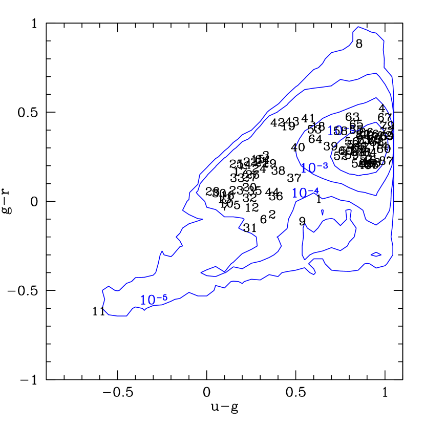
Figure 7: Colors $u-g$ vs. $g-r$ of the 87 Primary SDSS Early Data Release and RASS detected objects. Contours show the density of objects in our color-color diagram area that do not have RASS detections (i.e., the background object locus). Candidate objects are plotted by their ordering from Table 2. Magnitudes are PSF and reddening corrected.

Relaxing the third criterion (RASS detection), about 150,000 objects were returned. A number density of these objects was computed and plotted as a contour with logarithmically spaced density contours. See Fig. 7 for plots of the candidate objects against the background object density contours.

Of those 150,000 objects that fall within our color selection region, 2939 have been targeted spectroscopically. As noted in Heckler & Kolb (1996), it is possible for RBHs to fall in the QSO selection region and have spectra taken of them. Since they are not quasars (or any other type of known object), they would not be identified on the basis of these spectra and would be classified as unknown (in the SDSS database). In the 2939 that have spectra, 1877 have been classified as stars, 37 as galaxies, 996 as QSOs, and 29 as unknown. We list those 29 “unknown” objects in Table 3. Six of those 29 objects were later identifed as 5 QSOs and 1 WD. Note that object #18 in Table 3 is the same as object #3 in Table 2.

As seen in Fig. 6, our selection region intersect substantially with the loci of “normal” stars, white dwarves and QSOs (these we refer to as background objects). It is therefore not surprising that we will obtain these objects in our search, considering both that they themselves can be X-ray active and the possibility of “accidental” identification with a RASS source. Indeed, from Fig. 7 it appears that most of our candidates fall on the background loci.

In order to find those objects in our candidate list which are less likely to be background (star, QSO, etc.), we compute the relative overdensity $\eta$ of our candidate objects in the 4D color space. The 4D space is first split up into hypercubic bins of side length 0.25 magnitudes. The 87 candidate (RASS cut) objects and 156,563 (no RASS cut) background objects are then histogrammed. For every bin in which there is a candidate object, the overdensity for that object is given by

$$\eta=\left(\frac{\textrm{\# candidate objects in bin}}{\textrm{\# background objects in bin}}\right)\left(\frac{156,563}{87}\right)$$ (30)

Note that since every candidate object also appears as a background object, this overdensity has a maximum value of 156,563/87 $\sim$ 1800.

Using the synthetic object colors from Fan (1999) (and as noted earlier, from Fig. 6), we see that our color selection will pick up (at least) “normal” stars, QSOs of $z\lesssim 3$, WDs and Compact Emission Line Galaxies (CELGs). Given this fact, and the large “accidental” RASS identification rate computed in the last section, we might have expected the RASS selection to effectively be a random sampling of the background objects. To demonstrate this, 10 realizations of a random sampling of 87 objects from the background (of 156,563) objects was performed, and the subsequent values of $\eta$ are plotting in Fig. 8. As expected, most fall around $\eta\approx 1$ with some upwards scatter. Also plotted are the values of $\eta$ for our 87 candidates. Given the difference between the two populations, this implies that the RASS selection is not dominated by “accidental” identifications. In fact, note that QSOs appear to be preferentially selected by requiring a RASS detection, as RBHs hopefully will be as well. This alleviates, to some extent, some worry about our candidate list being dominated by “contaminant” objects.

We may, however, further attempt to rule out QSOs and CELGs as contaminants by looking for proper motion among our candidate objects. Being extragalactic objects, QSOs and CELGs will have no detectable proper motion.

The proper motion $\pi$ is given by

$$\pi\approx\frac{v}{d}\sin\theta$$ (31)

where $\theta$ is the angle between the RBH velocity $v$ and the line of sight. To compute typical proper motions, we first need typical velocities and distances;

$$\bar{v}=\int v\phi_{v}(v)dv=1.6\sigma$$ (32)

To compute a typical distance, we first compute the number density of RBHs.

$$n_{RBH} = \int\phi_{M}(M)dM$$ (33)

$$= \frac{f\rho_{DM}}{M_{\odot}I(x)}\int_{\mu_{min}}^{\mu_{max}}d\mu\mu^{-(1+x)}$$

$$= f\left(\frac{\rho_{DM}}{M_{\odot}}\right)\frac{I^{\prime\prime}(x)}{I(x)}$$

$$= 5.15\times 10^{-4}\textrm{ pc}^{-3}\left(\frac{f}{0.3}\right)\left(\frac{\rho_{DM}}{0.01M_{\odot}\textrm{ pc}^{-3}}\right)$$

Compare this with the value $8.0\times 10^{-4}$ pc^-3 computed by Shapiro & Teukolsky (1983) using a Salpeter initial mass function.

Taking a typical separation distance $d_{sep}=n_{RBH}^{-1/3}$,

$$d_{sep}=12.5\textrm{ pc}\left(\frac{f}{0.3}\right)^{-1/3}\left(\frac{\rho_{DM}}{0.01M_{\odot}\textrm{ pc}^{-3}}\right)^{-1/3}$$ (34)

Putting this into equation (31),

$$\pi=(1075\textrm{ mas yr}^{-1})\sin\theta\left(\frac{\bar{v}}{1.6\sigma}\right)\left(\frac{\sigma}{40\textrm{ km s}^{-1}}\right)\left(\frac{d}{12.5\textrm{ pc}}\right)^{-1}$$ (35)

Taking an RBH at the limit of detection (at a distance from equation (29)),

$$\pi=(17.4\textrm{ mas yr}^{-1})\sin\theta\left(\frac{M}{M_{\odot}}\right)^{-1}\left(\frac{v}{c_{s}}\right)\left[1+\left(\frac{v}{c_{s}}\right)^{2}\right]^{3/4}$$ (36)

The proper motion for this latter case rises more than linearly in velocity because in order to be detected, higher velocity RBHs need to be closer to us than lower velocity RBHs.

Given these estimates, we can search the USNO-A2.0 survey (Monet et al., 1998), which is also cross-listed with the SDSS EDR. The USNO survey was obtained from digitizing the photographic plates of the Palomar Optical Sky Survey (from 1953), and thus provides an opportunity to measure proper motion. Objects from the SDSS and USNO catalog are identified in the EDR database solely by requiring $\delta<$ 30”, where $\delta$ is the positional difference between the SDSS and USNO object. As the USNO data do not go as faint as the SDSS, there will be accidental matches to faint SDSS objects. Further, due to astronometric inaccuracies in the USNO survey, only matches with $\delta>$ 1” are included as candidates for proper motion (Hugh Harris, private communication). Note that these bounds on $\delta\in(1,30)^{\prime\prime}$ provide a corresponding bound on the proper motion $\pi\in(23,683)$ mas yr^-1. Accidental matches can further be reduced by comparing the blue and red magnitudes from the USNO object to the SDSS $g$ and $r$ magnitudes and requiring that they not be too disparate.

Table 4 lists those objects from the X-ray selected and spectroscopically selected candidates which may have proper motion.

6 Conclusions

Our basic result can be found in Tables 2 and 3: the 55 X-ray selected and 18 spectroscopically selected candidates for nearby, isolated, accreting black holes. The X-ray selected candidates have been ranked by $\eta$, the object overdensity in color-color space to identify those objects most likely to be RBHs. Given the number of candidates we have obtained, we return to equation (28) to see if this number is reasonable.

The factor of $10^{6}f$ in equation (28) assumes a solid-angle coverage of $\Omega_{SDSS}=\pi$. The Early Data Release covers $462\ \textrm{deg}^{2}$, or about 4.5% of $\pi$ steradians, and the relevant coefficient is $4.5\times 10^{4}f$ instead of $10^{6}f$.

Note that this value ($4.5\times 10^{4}f$) of represents the total number of RBH’s observed within the SDSS EDR, not those expected to be found with our search strategy. Since we require a RASS detection to be considered a candidate, the expected number is the smaller of $N_{SDSS}$ and $N_{RASS}$ for the sky coverage of the EDR. Using equation 28, we can compute the expected $N_{RASS}$ as follows.

Using an ADAF spectral model (which the value of $N_{SDSS}$ in equation 28 assumes), $f_{RASS}\approx 10^{-2}f_{SDSS}\approx 5\times 10^{-4}$. Using $F_{RASS}^{min}=10^{-13}$ erg cm^-2 s^-1, this gives $4f$ RBH’s over the entire sky or $0.045f$ within the EDR. This value of $F_{RASS}^{min}$ is actually an overestimate by about an order of magnitude, given observed sources with count rates below the limit. In this case, $N_{RASS}$ within the EDR rises by a factor of 10^3/2 to $1.4f$.

Using a CDAF model instead, the RBH becomes more luminous in the X-ray than in the optical ($f_{RASS}>f_{SDSS}$). If we assume that $f_{SDSS}=5\times 10^{-4}$, then $N_{SDSS}$ within the EDR becomes $45f$. Given $F_{RASS}^{min}=10^{-14}$ erg cm^-2 s^-1 and $f_{RASS}=5\times 10^{-2}$, $N_{RASS}$ within the EDR becomes $4500f$.

The above estimates still do not represent the expected number of candidates until a value of $f$ is specified. The value of $\rho_{DM}$ represents the local value of the galactic dark matter halo. Recent microlensing work by Lasserre et al. (2000) indicates that the halo may be made of of compact objects if their mass is greater than 1 $M_{\odot}$. Venkatesan, Olinto & Truran (1999) place a limit of $f\lesssim 0.3-0.4$ by requiring that the RBH progenitor population of stars not overenrich the galaxy with metals.

The next step in the program would be follow-up observations of the 57 remaining candidates. Spectroscopic determination of stellar or QSO-like spectra would rule out the candidate. Higher resolution X-ray observations would confirm X-ray emission. Determination of variability either in optical or X-ray, or any indication of proper motion would make the candidate source very interesting.

Of the three methods of detecting isolated RBH mentioned earlier, only one (microlensing) has possibly been successful. This, however, does not decrease the need for detecting accretion emission. As microlensing uses the magnification of light as an object passes between source and observer, it is most sensitive to high-velocity black holes. Since the accretion luminosity scales as $L\propto\dot{M}\propto v^{-3}$, it would be expected that a RBH detected in microlensing would not be detected through its emission [see Revnivtsev & Sunyaev (2001)]. Thus these two methods are complementary, as those RBH with low $v$ would not be detectable with microlensing but more likely through accretion.

It should be noted that the three methods for detecting RBH’s are not as sensitive to primordial black holes. Detection through supernova light curves is obviously out. Since $L\propto\dot{M}\propto M^{2}$, black holes with masses much lighter than solar become undetectable through accretion emission. Similarly for microlensing, the peak magnification scales as $A\propto M^{1/2}$.

Finally we turn to limits on the contribution of RBHs to the local dark-matter density. Of course any limit is only as reliable as the assumptions used to derive it. In this case, the major uncertainty is the source spectrum. Nevertheless, if we assume that all 55 of the non-identified sources in Table 2 are sources, then using equation (28) with the coefficient appropriate for the SDSS Early Data Release ($4.5\times 10^{4}f$ rather than $10^{6}f$) the limit on the contribution of remnant black holes is $10^{-3}$ of the dark matter density. Of course there are many assumptions that are behind this limit. It assumes that the spectral energy density is given by ADAF models, and that all possible SDSS sources would have been seen in the RASS. For these reasons, we view this work as a search for isolated, stellar-mass black holes, rather than an attempt to place a limit on their contribution to local dark matter.

During the writing of this paper, one of our X-ray selected candidates, # 21, was observed spectroscopically to be a $z=0.927$ QSO. We thank Mike Brotherton and Paul Nandra for bringing this to our attention and providing the spectrum.

Figure 1: Sample models for the spectral energy distribution of a $10M_{\odot}$ black hole accreting from the ISM. The solid line is an ADAF model, the dotted line is an IP model, and the dashed line is a CDAF model. The curves are meant to show the major spectral differences between the models. The integrated luminosity of all three models is $\epsilon\dot{M}$, where $\dot{M}=2.5\times 10^{32}\ \textrm{erg s}^{-1}$ is the mass accretion rate for a hole of mass $10M_{\odot}$ and velocity of $40\ \textrm{km s}^{-1}$.

Figure 2: The SDSS transmission curves in the five filter bands, including atmospheric effects (airmass of 1.3), from Stoughton et al. (2002).

Figure 4: The tracks of a pure power law (solid line) and broken power law (asterisks) synthetic spectra. The numbers indicate the power law slope at that point on the curve. We expect the color of RBH’s to fall somewhere in the shaded triangular region above.

Figure 5: This figure shows how the SDSS colors change with peak frequency. The assumed spectrum is a broken power law, changing from $+2$ to $-3$.

Figure 6: A sample of 43708 “stars” from the Early Data Release in a 10^o slice in RA. Noted are the positions of the stellar, QSO and WD loci.

Figure 8: The candidate object overdensity $\eta$; small blue dots are overdensities from 10 random samples of 87 objects from the background (none of these 870 random objects are necessarily our candidates). The 87 candidates are plotted (in no particular order) by spectral type, if known: Unknown (not targeted), Star, or QSO.

Table 1: SDSS Filter Characteristics

Band	$\nu_{\textrm{min}}$ (1014 Hz)	$\bar{\nu}$ (1014 Hz)	$\nu_{\textrm{max}}$ (1014 Hz)	95% completeness limit	$F_{\alpha}^{min}$ (10-15 ergs s-1 cm-2)
$u$	8	8.57	9	22.0	0.89
$g$	5.5	6.25	7	22.2	3.53
$r$	4.25	4.80	5.25	22.2	2.66
$i$	3.75	3.90	4.25	21.3	3.59
$z$	3	3.30	3.5	20.5	1.39

Note. — The average wavelengths, frequencies, completeness limits, and corresponding limiting fluxes for the SDSS photometric filters. The 95% completeness limit is for point sources, from Stoughton et al. (2002).

Table 2: X-ray selected remnant black hole candidates.

#	RA	dec	$u^{*}$	$g^{*}$	$r^{*}$	$i^{*}$	$z^{*}$	RASS	$\eta$
1	01 55 43.4	00 28 07.2	15.90 $\pm$ 0.02	15.27 $\pm$ 0.01	15.25 $\pm$ 0.02	15.51 $\pm$ 0.01	15.69 $\pm$ 0.01	42 $\pm$ 12	1799.6
2	17 34 25.5	60 39 37.8	19.74 $\pm$ 0.05	19.37 $\pm$ 0.02	19.44 $\pm$ 0.02	19.40 $\pm$ 0.03	19.66 $\pm$ 0.08	6 $\pm$ 2	1799.6
3	13 11 06.5	00 35 10.1	18.37 $\pm$ 0.01	18.04 $\pm$ 0.02	17.78 $\pm$ 0.01	17.57 $\pm$ 0.02	17.32 $\pm$ 0.02	105 $\pm$ 24	128.5
4	15 07 38.0	00 18 51.4	18.16 $\pm$ 0.02	17.17 $\pm$ 0.03	16.65 $\pm$ 0.01	16.53 $\pm$ 0.01	16.81 $\pm$ 0.05	18 $\pm$ 9	112.5
5	00 10 47.5	00 19 00.4	18.92 $\pm$ 0.02	18.75 $\pm$ 0.01	18.77 $\pm$ 0.02	18.74 $\pm$ 0.02	18.73 $\pm$ 0.06	18 $\pm$ 9	105.9
6	11 45 10.4	01 10 56.2	19.28 $\pm$ 0.03	18.96 $\pm$ 0.01	19.06 $\pm$ 0.01	19.01 $\pm$ 0.02	19.00 $\pm$ 0.05	26 $\pm$ 12	105.9
7	11 52 46.6	00 24 40.0	17.63 $\pm$ 0.01	17.53 $\pm$ 0.02	17.56 $\pm$ 0.01	17.53 $\pm$ 0.01	17.47 $\pm$ 0.02	27 $\pm$ 11	105.9
8	17 09 21.6	57 06 24.0	21.85 $\pm$ 0.18	21.00 $\pm$ 0.04	20.11 $\pm$ 0.02	19.61 $\pm$ 0.03	19.13 $\pm$ 0.06	9 $\pm$ 3	105.9
9	00 34 43.9	$-$00 54 13.1	19.59 $\pm$ 0.03	19.05 $\pm$ 0.03	19.16 $\pm$ 0.02	19.12 $\pm$ 0.03	19.07 $\pm$ 0.06	37 $\pm$ 10	69.2
10	17 19 36.7	60 47 48.1	18.84 $\pm$ 0.03	18.73 $\pm$ 0.01	18.74 $\pm$ 0.01	18.80 $\pm$ 0.02	18.72 $\pm$ 0.04	14 $\pm$ 4	45.0
11	11 46 35.2	00 12 33.5	14.17 $\pm$ 0.01	14.78 $\pm$ 0.02	15.39 $\pm$ 0.02	15.77 $\pm$ 0.02	16.12 $\pm$ 0.03	91 $\pm$ 20	43.9
12	16 49 31.1	64 21 31.0	19.14 $\pm$ 0.03	18.89 $\pm$ 0.02	18.92 $\pm$ 0.02	18.88 $\pm$ 0.02	18.90 $\pm$ 0.05	4 $\pm$ 2	35.3
13	15 26 14.5	$-$00 44 45.2	18.27 $\pm$ 0.02	18.17 $\pm$ 0.01	18.15 $\pm$ 0.02	18.23 $\pm$ 0.01	18.19 $\pm$ 0.02	17 $\pm$ 7	33.3
14	13 51 28.3	01 03 38.6	17.37 $\pm$ 0.01	17.16 $\pm$ 0.02	16.95 $\pm$ 0.02	16.95 $\pm$ 0.01	17.01 $\pm$ 0.02	40 $\pm$ 13	31.3
15	17 32 58.8	59 35 12.0	19.74 $\pm$ 0.04	19.45 $\pm$ 0.02	19.22 $\pm$ 0.02	19.36 $\pm$ 0.02	19.44 $\pm$ 0.07	6 $\pm$ 2	31.3
16	17 00 35.4	63 25 22.7	18.15 $\pm$ 0.02	18.03 $\pm$ 0.02	18.00 $\pm$ 0.06	18.05 $\pm$ 0.02	18.09 $\pm$ 0.03	4 $\pm$ 2	31.3
17	10 18 27.1	-00 00 08.5	19.54 $\pm$ 0.03	19.35 $\pm$ 0.01	19.19 $\pm$ 0.02	19.25 $\pm$ 0.02	19.42 $\pm$ 0.06	26 $\pm$ 10	31.3
18	17 23 58.0	60 11 40.1	19.72 $\pm$ 0.03	19.09 $\pm$ 0.02	18.67 $\pm$ 0.02	18.34 $\pm$ 0.02	17.99 $\pm$ 0.03	10 $\pm$ 3	28.6
19	11 32 45.6	00 34 27.8	18.28 $\pm$ 0.02	17.82 $\pm$ 0.01	17.40 $\pm$ 0.01	17.09 $\pm$ 0.02	16.77 $\pm$ 0.01	19 $\pm$ 9	24.7
20	09 48 57.3	00 22 25.5	18.61 $\pm$ 0.02	18.37 $\pm$ 0.01	18.29 $\pm$ 0.01	18.13 $\pm$ 0.01	18.16 $\pm$ 0.03	41 $\pm$ 11	21.3
21	17 14 38.6	61 50 39.4	20.07 $\pm$ 0.05	19.76 $\pm$ 0.02	19.54 $\pm$ 0.02	19.50 $\pm$ 0.03	19.62 $\pm$ 0.08	8 $\pm$ 3	21.3
22	17 10 30.2	60 23 47.6	18.01 $\pm$ 0.02	17.76 $\pm$ 0.02	17.54 $\pm$ 0.01	17.30 $\pm$ 0.02	17.38 $\pm$ 0.02	12 $\pm$ 4	21.3
23	13 54 25.2	$-$00 13 58.0	16.82 $\pm$ 0.02	16.65 $\pm$ 0.01	16.59 $\pm$ 0.01	16.44 $\pm$ 0.01	16.45 $\pm$ 0.02	39 $\pm$ 13	21.3
24	11 10 34.5	$-$01 05 17.5	20.44 $\pm$ 0.07	20.15 $\pm$ 0.03	19.96 $\pm$ 0.03	19.73 $\pm$ 0.03	19.80 $\pm$ 0.10	16 $\pm$ 9	21.3
25	00 35 34.2	$-$00 25 48.8	19.51 $\pm$ 0.03	19.35 $\pm$ 0.02	19.14 $\pm$ 0.02	19.11 $\pm$ 0.02	19.35 $\pm$ 0.08	20 $\pm$ 8	21.3
26	12 13 47.5	00 01 30.0	18.28 $\pm$ 0.01	18.02 $\pm$ 0.03	17.87 $\pm$ 0.03	17.89 $\pm$ 0.02	17.86 $\pm$ 0.02	39 $\pm$ 15	18.5
27	17 20 28.8	65 19 40.2	19.36 $\pm$ 0.03	19.12 $\pm$ 0.02	18.98 $\pm$ 0.02	19.07 $\pm$ 0.02	19.04 $\pm$ 0.06	5 $\pm$ 2	18.5
28	17 23 16.2	53 36 31.2	19.07 $\pm$ 0.02	19.04 $\pm$ 0.01	18.98 $\pm$ 0.02	19.05 $\pm$ 0.04	19.18 $\pm$ 0.07	8 $\pm$ 3	16.4
29	17 08 32.2	62 42 05.8	19.12 $\pm$ 0.02	18.77 $\pm$ 0.01	18.55 $\pm$ 0.03	18.57 $\pm$ 0.02	18.66 $\pm$ 0.04	9 $\pm$ 3	14.5
30	12 10 16.1	00 12 04.9	17.03 $\pm$ 0.01	16.96 $\pm$ 0.02	16.92 $\pm$ 0.01	16.86 $\pm$ 0.01	16.92 $\pm$ 0.04	18. $\pm$ 9	12.1
31	03 09 11.6	00 23 58.9	16.94 $\pm$ 0.02	16.70 $\pm$ 0.01	16.84 $\pm$ 0.01	16.89 $\pm$ 0.01	17.02 $\pm$ 0.02	59 $\pm$ 18	9.0
32	11 37 49.8	00 27 35.3	17.50 $\pm$ 0.01	17.26 $\pm$ 0.02	17.24 $\pm$ 0.03	17.20 $\pm$ 0.01	17.08 $\pm$ 0.03	33 $\pm$ 13	8.4
33	17 15 08.1	55 29 25.0	17.93 $\pm$ 0.02	17.76 $\pm$ 0.02	17.63 $\pm$ 0.02	17.62 $\pm$ 0.02	17.59 $\pm$ 0.02	11 $\pm$ 4	8.4
34	17 20 52.3	57 55 13.2	20.52 $\pm$ 0.06	20.21 $\pm$ 0.05	19.98 $\pm$ 0.05	19.93 $\pm$ 0.09	19.81 $\pm$ 0.12	14 $\pm$ 4	8.4
35	17 22 40.1	61 05 60.0	19.37 $\pm$ 0.03	19.10 $\pm$ 0.01	19.04 $\pm$ 0.02	19.01 $\pm$ 0.02	18.86 $\pm$ 0.05	12 $\pm$ 3	8.4
36	00 59 18.2	00 25 19.7	18.45 $\pm$ 0.02	18.06 $\pm$ 0.02	18.03 $\pm$ 0.01	17.96 $\pm$ 0.01	17.90 $\pm$ 0.03	46 $\pm$ 14	7.7
37	17 45 04.4	53 20 27.5	19.35 $\pm$ 0.03	18.86 $\pm$ 0.02	18.73 $\pm$ 0.01	18.62 $\pm$ 0.02	18.43 $\pm$ 0.03	11 $\pm$ 3	7.7
38	01 46 01.7	$-$00 21 22.0	20.41 $\pm$ 0.08	20.01 $\pm$ 0.02	19.84 $\pm$ 0.02	19.68 $\pm$ 0.02	19.46 $\pm$ 0.07	18 $\pm$ 8	7.7
39	11 54 12.0	01 00 57.6	21.15 $\pm$ 0.16	20.45 $\pm$ 0.04	20.14 $\pm$ 0.03	19.95 $\pm$ 0.07	19.68 $\pm$ 0.12	33 $\pm$ 12	5.7
40	17 14 30.1	61 57 46.6	19.90 $\pm$ 0.05	19.39 $\pm$ 0.02	19.09 $\pm$ 0.02	19.00 $\pm$ 0.02	18.86 $\pm$ 0.05	17 $\pm$ 4	5.2
41	17 33 49.7	58 43 57.6	21.74 $\pm$ 0.18	21.17 $\pm$ 0.04	20.70 $\pm$ 0.04	20.57 $\pm$ 0.05	20.42 $\pm$ 0.15	7 $\pm$ 2	5.2
42	12 03 46.6	$-$00 17 23.1	19.98 $\pm$ 0.05	19.58 $\pm$ 0.03	19.14 $\pm$ 0.02	19.08 $\pm$ 0.02	19.06 $\pm$ 0.07	26 $\pm$ 11	5.2
43	11 04 54.8	$-$01 08 53.4	20.86 $\pm$ 0.10	20.38 $\pm$ 0.03	19.93 $\pm$ 0.03	19.76 $\pm$ 0.04	19.61 $\pm$ 0.08	16 $\pm$ 8	5.2
44	17 09 56.0	57 32 25.5	18.63 $\pm$ 0.02	18.26 $\pm$ 0.01	18.21 $\pm$ 0.01	18.09 $\pm$ 0.02	18.10 $\pm$ 0.04	28 $\pm$ 5	5.0
45	13 31 11.1	01 00 12.3	20.61 $\pm$ 0.06	19.72 $\pm$ 0.03	19.51 $\pm$ 0.03	19.43 $\pm$ 0.04	19.32 $\pm$ 0.07	30 $\pm$ 12	1.1
46	12 14 42.0	00 40 17.5	20.63 $\pm$ 0.05	19.72 $\pm$ 0.02	19.49 $\pm$ 0.02	19.39 $\pm$ 0.02	19.37 $\pm$ 0.05	24 $\pm$ 11	1.1
47	17 25 32.1	57 16 35.4	20.83 $\pm$ 0.09	19.91 $\pm$ 0.02	19.70 $\pm$ 0.02	19.51 $\pm$ 0.03	19.43 $\pm$ 0.07	27 $\pm$ 6	1.1
48	17 31 00.4	57 22 12.4	19.10 $\pm$ 0.03	18.16 $\pm$ 0.02	17.94 $\pm$ 0.01	17.81 $\pm$ 0.02	17.62 $\pm$ 0.02	8 $\pm$ 3	1.1
49	15 24 37.1	00 18 46.2	18.94 $\pm$ 0.03	18.04 $\pm$ 0.02	17.82 $\pm$ 0.02	17.77 $\pm$ 0.01	17.71 $\pm$ 0.03	23 $\pm$ 11	1.1
50	15 13 45.0	00 18 20.7	19.57 $\pm$ 0.03	18.72 $\pm$ 0.01	18.51 $\pm$ 0.01	18.43 $\pm$ 0.01	18.36 $\pm$ 0.03	23 $\pm$ 10	1.1
51	12 50 28.1	$-$00 46 56.5	18.64 $\pm$ 0.02	17.74 $\pm$ 0.01	17.50 $\pm$ 0.03	17.39 $\pm$ 0.02	17.36 $\pm$ 0.02	45 $\pm$ 19	1.1
52	12 14 41.4	00 40 32.9	21.41 $\pm$ 0.09	20.66 $\pm$ 0.02	20.41 $\pm$ 0.03	20.28 $\pm$ 0.03	20.39 $\pm$ 0.11	24 $\pm$ 11	0.9
53	12 15 25.1	00 53 16.9	20.94 $\pm$ 0.10	20.34 $\pm$ 0.03	19.94 $\pm$ 0.03	19.93 $\pm$ 0.04	19.95 $\pm$ 0.12	26 $\pm$ 11	0.9
54	16 59 50.8	62 38 45.5	21.03 $\pm$ 0.11	20.20 $\pm$ 0.02	19.88 $\pm$ 0.02	19.64 $\pm$ 0.03	19.71 $\pm$ 0.10	6 $\pm$ 2	0.9
55	23 47 25.2	$-$01 06 36.0	20.35 $\pm$ 0.08	19.51 $\pm$ 0.02	19.11 $\pm$ 0.02	18.97 $\pm$ 0.02	18.99 $\pm$ 0.06	48 $\pm$ 14	0.9
56	10 47 20.6	$-$00 41 48.3	21.32 $\pm$ 0.15	20.50 $\pm$ 0.04	20.17 $\pm$ 0.04	20.03 $\pm$ 0.04	20.25 $\pm$ 0.16	42 $\pm$ 12	0.9
57	17 11 22.3	58 04 60.0	20.94 $\pm$ 0.08	20.15 $\pm$ 0.03	19.86 $\pm$ 0.03	19.75 $\pm$ 0.02	19.58 $\pm$ 0.08	10 $\pm$ 4	0.8
58	17 15 24.3	55 00 14.1	21.78 $\pm$ 0.19	21.03 $\pm$ 0.05	20.63 $\pm$ 0.04	20.43 $\pm$ 0.05	20.23 $\pm$ 0.14	10 $\pm$ 4	0.8
59	17 15 34.2	63 23 45.5	20.45 $\pm$ 0.08	19.64 $\pm$ 0.02	19.38 $\pm$ 0.02	19.27 $\pm$ 0.02	19.18 $\pm$ 0.07	6 $\pm$ 2	0.8
60	17 06 05.9	64 38 20.2	20.76 $\pm$ 0.09	19.98 $\pm$ 0.03	19.70 $\pm$ 0.02	19.58 $\pm$ 0.03	19.56 $\pm$ 0.09	6 $\pm$ 2	0.8
61	17 31 34.2	59 13 52.7	18.49 $\pm$ 0.02	17.65 $\pm$ 0.01	17.37 $\pm$ 0.01	17.30 $\pm$ 0.01	17.29 $\pm$ 0.02	4 $\pm$ 2	0.8
62	15 16 57.1	$-$00 37 24.6	19.09 $\pm$ 0.02	18.24 $\pm$ 0.02	17.95 $\pm$ 0.01	17.84 $\pm$ 0.02	17.81 $\pm$ 0.02	176 $\pm$ 32	0.8
63	14 37 37.5	$-$00 20 07.5	22.17 $\pm$ 0.19	21.36 $\pm$ 0.04	20.88 $\pm$ 0.04	20.77 $\pm$ 0.04	20.68 $\pm$ 0.16	85 $\pm$ 23	0.8
64	02 25 07.9	$-$00 35 33.0	19.44 $\pm$ 0.03	18.83 $\pm$ 0.01	18.48 $\pm$ 0.02	18.33 $\pm$ 0.02	18.12 $\pm$ 0.04	70 $\pm$ 20	0.8
65	01 04 14.9	$-$00 24 34.0	21.41 $\pm$ 0.16	20.57 $\pm$ 0.03	20.14 $\pm$ 0.03	19.94 $\pm$ 0.03	19.77 $\pm$ 0.12	21 $\pm$ 9	0.8
66	17 24 11.7	57 17 28.4	20.91 $\pm$ 0.09	20.01 $\pm$ 0.03	19.62 $\pm$ 0.02	19.46 $\pm$ 0.02	19.48 $\pm$ 0.07	8 $\pm$ 3	0.6
67	16 49 36.7	64 28 15.2	21.43 $\pm$ 0.13	20.43 $\pm$ 0.03	19.96 $\pm$ 0.02	19.72 $\pm$ 0.03	19.86 $\pm$ 0.11	41 $\pm$ 6	0.6
68	16 58 53.7	63 27 51.8	20.94 $\pm$ 0.09	20.08 $\pm$ 0.02	19.77 $\pm$ 0.04	19.77 $\pm$ 0.03	19.85 $\pm$ 0.11	3 $\pm$ 1	0.6
69	17 24 08.2	64 49 24.4	17.62 $\pm$ 0.02	16.61 $\pm$ 0.01	16.24 $\pm$ 0.02	16.10 $\pm$ 0.01	16.10 $\pm$ 0.02	5 $\pm$ 2	0.6
70	14 37 30.6	$-$00 21 16.5	18.28 $\pm$ 0.01	17.35 $\pm$ 0.01	17.00 $\pm$ 0.01	16.88 $\pm$ 0.01	16.89 $\pm$ 0.02	26 $\pm$ 11	0.6
71	11 04 54.7	$-$01 09 11.9	20.00 $\pm$ 0.06	19.09 $\pm$ 0.02	18.78 $\pm$ 0.02	18.73 $\pm$ 0.03	18.76 $\pm$ 0.04	16 $\pm$ 8	0.6
72	00 17 25.5	$-$01 11 51.4	19.56 $\pm$ 0.04	18.56 $\pm$ 0.01	18.19 $\pm$ 0.02	18.10 $\pm$ 0.01	18.11 $\pm$ 0.03	22 $\pm$ 10	0.6
73	01 31 44.7	00 33 04.9	19.80 $\pm$ 0.04	18.92 $\pm$ 0.02	18.58 $\pm$ 0.01	18.47 $\pm$ 0.02	18.40 $\pm$ 0.03	46 $\pm$ 14	0.4
74	13 56 15.4	00 03 58.1	18.93 $\pm$ 0.02	17.95 $\pm$ 0.01	17.64 $\pm$ 0.02	17.51 $\pm$ 0.01	17.50 $\pm$ 0.02	24 $\pm$ 11	0.4
75	17 23 57.3	58 33 08.1	20.78 $\pm$ 0.10	19.81 $\pm$ 0.02	19.44 $\pm$ 0.02	19.33 $\pm$ 0.02	19.25 $\pm$ 0.06	13 $\pm$ 4	0.4
76	17 27 00.6	58 19 17.1	20.78 $\pm$ 0.10	19.86 $\pm$ 0.03	19.48 $\pm$ 0.02	19.24 $\pm$ 0.02	19.17 $\pm$ 0.05	8 $\pm$ 4	0.4
77	17 24 03.1	52 53 45.6	21.53 $\pm$ 0.12	20.51 $\pm$ 0.03	20.12 $\pm$ 0.03	19.99 $\pm$ 0.04	19.86 $\pm$ 0.11	10 $\pm$ 4	0.4
78	15 35 58.5	00 03 39.6	17.44 $\pm$ 0.01	16.56 $\pm$ 0.01	16.28 $\pm$ 0.01	16.20 $\pm$ 0.01	16.18 $\pm$ 0.02	22 $\pm$ 8	0.4
79	15 32 53.3	$-$00 46 02.5	19.39 $\pm$ 0.04	18.38 $\pm$ 0.02	17.96 $\pm$ 0.02	17.75 $\pm$ 0.01	17.69 $\pm$ 0.02	27 $\pm$ 11	0.4
80	14 31 19.3	$-$00 54 37.2	19.61 $\pm$ 0.03	18.62 $\pm$ 0.01	18.33 $\pm$ 0.01	18.25 $\pm$ 0.01	18.24 $\pm$ 0.03	40 $\pm$ 14	0.4
81	13 04 27.0	$-$00 35 41.6	19.22 $\pm$ 0.02	18.34 $\pm$ 0.02	17.99 $\pm$ 0.02	17.81 $\pm$ 0.01	17.73 $\pm$ 0.02	30 $\pm$ 14	0.4
82	12 50 23.6	$-$00 47 49.0	19.42 $\pm$ 0.03	18.54 $\pm$ 0.02	18.17 $\pm$ 0.03	17.96 $\pm$ 0.02	17.92 $\pm$ 0.03	45 $\pm$ 19	0.4
83	13 14 41.2	$-$01 07 01.5	18.73 $\pm$ 0.02	17.78 $\pm$ 0.02	17.44 $\pm$ 0.02	17.32 $\pm$ 0.01	17.26 $\pm$ 0.02	32 $\pm$ 14	0.4
84	11 40 24.7	$-$00 59 26.7	19.79 $\pm$ 0.03	18.88 $\pm$ 0.01	18.60 $\pm$ 0.01	18.48 $\pm$ 0.01	18.43 $\pm$ 0.03	60 $\pm$ 22	0.4
85	11 40 28.4	$-$00 15 51.2	19.26 $\pm$ 0.03	18.32 $\pm$ 0.02	17.98 $\pm$ 0.01	17.85 $\pm$ 0.02	17.79 $\pm$ 0.03	36 $\pm$ 15	0.4
86	12 12 22.8	00 25 46.9	19.90 $\pm$ 0.04	18.97 $\pm$ 0.02	18.77 $\pm$ 0.01	18.69 $\pm$ 0.03	18.69 $\pm$ 0.05	20 $\pm$ 9	0.4
87	16 56 22.4	64 35 43.6	20.73 $\pm$ 0.08	19.72 $\pm$ 0.03	19.49 $\pm$ 0.02	19.41 $\pm$ 0.03	19.44 $\pm$ 0.08	4 $\pm$ 2	0.4

Note. — Positions are J2000. SDSS magnitudes $u^{*}$, $g^{*}$, $r^{*}$, $i^{*}$, $z^{*}$ are reddening corrected point-spread-function (PSF) magnitudes. The RASS count rate is in counts ksec^-1. All errors are 1-$\sigma$. The overdensity $\eta$ is defined in equation (30), and is used to rank those candidates most likely to be RBHs.

Table 3: Spectroscopically selected remnant black hole candidates.

#	RA	dec	$u^{*}$	$g^{*}$	$r^{*}$	$i^{*}$	$z^{*}$	Plate	MJD	Fiber
1	01 00 58.2	-00 55 47.9	19.68 $\pm$ 0.03	19.17 $\pm$ 0.02	18.76 $\pm$ 0.02	18.36 $\pm$ 0.02	18.10 $\pm$ 0.03	395	51783	18
2	01 27 23.6	-00 46 30.1	18.79 $\pm$ 0.02	18.59 $\pm$ 0.01	18.71 $\pm$ 0.01	18.76 $\pm$ 0.02	18.85 $\pm$ 0.05	399	51817	99
3	03 16 42.7	-00 08 16.7	18.83 $\pm$ 0.02	18.85 $\pm$ 0.02	18.98 $\pm$ 0.02	19.20 $\pm$ 0.02	19.45 $\pm$ 0.10	412	51931	21
4	03 44 01.4	-00 12 21.0	19.26 $\pm$ 0.04	19.27 $\pm$ 0.01	19.49 $\pm$ 0.02	19.71 $\pm$ 0.03	19.89 $\pm$ 0.14	416	51811	111
5	03 42 26.3	-00 14 09.9	20.28 $\pm$ 0.08	20.13 $\pm$ 0.03	19.92 $\pm$ 0.04	19.93 $\pm$ 0.04	20.07 $\pm$ 0.15	416	51811	154
6	03 33 57.2	-00 11 06.1	19.78 $\pm$ 0.05	19.64 $\pm$ 0.02	19.55 $\pm$ 0.02	19.47 $\pm$ 0.02	19.42 $\pm$ 0.10	415	51810	174
7	10 32 43.3	-00 32 43.6	19.56 $\pm$ 0.03	19.86 $\pm$ 0.02	20.18 $\pm$ 0.02	20.52 $\pm$ 0.04	20.71 $\pm$ 0.18	273	51957	163
8	12 25 19.9	-01 07 36.9	20.11 $\pm$ 0.04	19.47 $\pm$ 0.02	19.10 $\pm$ 0.01	19.11 $\pm$ 0.02	19.11 $\pm$ 0.06	289	51990	250
9	15 24 40.1	00 32 52.1	19.47 $\pm$ 0.03	19.02 $\pm$ 0.01	18.73 $\pm$ 0.02	18.58 $\pm$ 0.01	18.43 $\pm$ 0.03	313	51673	463
10	17 43 52.5	54 54 38.8	20.50 $\pm$ 0.08	20.22 $\pm$ 0.03	20.37 $\pm$ 0.03	20.37 $\pm$ 0.05	20.39 $\pm$ 0.16	360	51816	633
11	17 11 01.5	65 45 49.9	19.18 $\pm$ 0.03	18.79 $\pm$ 0.02	18.68 $\pm$ 0.02	18.73 $\pm$ 0.02	18.90 $\pm$ 0.05	350	51691	367
12	17 33 27.3	58 54 39.8	19.95 $\pm$ 0.04	19.88 $\pm$ 0.02	19.98 $\pm$ 0.02	20.10 $\pm$ 0.04	20.16 $\pm$ 0.12	366	52017	582
13	17 09 27.5	62 29 01.5	19.14 $\pm$ 0.03	18.91 $\pm$ 0.01	18.84 $\pm$ 0.03	18.97 $\pm$ 0.04	19.02 $\pm$ 0.05	351	51780	580
14	17 24 11.5	58 37 10.9	20.70 $\pm$ 0.09	20.36 $\pm$ 0.02	20.34 $\pm$ 0.04	20.30 $\pm$ 0.04	20.23 $\pm$ 0.13	366	52017	280
15	17 22 28.9	58 40 10.9	19.76 $\pm$ 0.04	19.79 $\pm$ 0.02	20.11 $\pm$ 0.03	20.32 $\pm$ 0.05	20.40 $\pm$ 0.16	366	52017	434
16	17 33 42.9	55 44 19.1	18.86 $\pm$ 0.02	18.56 $\pm$ 0.02	18.57 $\pm$ 0.01	18.64 $\pm$ 0.01	18.71 $\pm$ 0.04	360	51816	380
17	17 24 00.7	57 35 38.2	20.22 $\pm$ 0.05	20.21 $\pm$ 0.02	20.40 $\pm$ 0.04	20.47 $\pm$ 0.05	20.68 $\pm$ 0.17	366	52017	248
18	13 11 06.5	00 35 10.1	18.37 $\pm$ 0.01	18.04 $\pm$ 0.02	17.78 $\pm$ 0.01	17.57 $\pm$ 0.02	17.32 $\pm$ 0.02	294	51986	629
19	12 55 59.6	00 51 06.0	20.54 $\pm$ 0.06	20.15 $\pm$ 0.02	20.05 $\pm$ 0.02	20.02 $\pm$ 0.03	19.90 $\pm$ 0.09	293	51689	372
20	14 44 54.6	00 42 24.5	21.34 $\pm$ 0.10	20.67 $\pm$ 0.03	20.22 $\pm$ 0.02	20.05 $\pm$ 0.04	19.82 $\pm$ 0.08	308	51662	414
21	11 47 37.9	00 13 01.0	21.91 $\pm$ 0.15	21.11 $\pm$ 0.03	20.35 $\pm$ 0.02	19.84 $\pm$ 0.03	19.25 $\pm$ 0.06	283	51959	543
22	11 10 07.6	01 10 41.6	18.03 $\pm$ 0.02	17.51 $\pm$ 0.02	17.36 $\pm$ 0.02	17.32 $\pm$ 0.01	17.35 $\pm$ 0.02	278	51900	523
23	03 38 10.9	00 56 17.7	20.19 $\pm$ 0.08	19.25 $\pm$ 0.02	18.40 $\pm$ 0.01	18.14 $\pm$ 0.01	18.28 $\pm$ 0.03	415	51810	617
24	03 33 20.4	00 07 20.6	16.56 $\pm$ 0.02	16.19 $\pm$ 0.01	16.17 $\pm$ 0.01	16.18 $\pm$ 0.01	16.37 $\pm$ 0.01	415	51810	492
25	01 07 48.2	01 02 40.7	19.09 $\pm$ 0.03	18.70 $\pm$ 0.02	18.49 $\pm$ 0.02	18.50 $\pm$ 0.01	18.50 $\pm$ 0.04	396	51816	571
26	02 51 11.7	00 29 15.1	19.38 $\pm$ 0.04	19.17 $\pm$ 0.02	19.31 $\pm$ 0.02	19.52 $\pm$ 0.03	19.60 $\pm$ 0.09	410	51816	347
27	02 58 29.0	00 15 26.1	20.39 $\pm$ 0.07	20.15 $\pm$ 0.02	19.97 $\pm$ 0.03	19.87 $\pm$ 0.03	19.65 $\pm$ 0.14	410	51816	559
28	01 47 33.6	00 03 23.3	18.68 $\pm$ 0.02	18.08 $\pm$ 0.01	17.70 $\pm$ 0.01	17.40 $\pm$ 0.02	17.23 $\pm$ 0.02	402	51793	400
29	02 13 03.8	00 38 11.9	21.04 $\pm$ 0.11	20.64 $\pm$ 0.03	20.13 $\pm$ 0.03	19.75 $\pm$ 0.03	19.46 $\pm$ 0.07	405	51816	469

Note. — Positions are J2000. SDSS magnitudes $u^{*}$, $g^{*}$, $r^{*}$, $i^{*}$, $z^{*}$ are reddening corrected point-spread-function (PSF) magnitudes. All errors are 1-$\sigma$. MJD is the Modified Julian Date of when the spectra was taken.

Table 4: Proper Motions

#	$\pi$	$\delta$	blue	red	$g^{*}$	$r^{*}$
X-1	62.6	2.82	18.2	16.5	15.38	15.32
X-39	24.3	1.15	19.6	18.9	20.56	20.25
X-44	31.6	1.42	17.9	18.3	18.40	18.33
X-70	32.6	1.43	17.0	16.7	17.49	17.10
X-72	25.2	1.19	18.4	17.8	18.77	18.34
X-81	34.9	1.50	18.3	17.9	18.37	18.02
X-85	26.8	1.26	18.1	17.7	18.47	18.11
S-2	97.9	4.30	17.8	18.6	18.67	18.76
S-11	80.4	3.77	18.6	18.8	18.89	18.76
S-22	406.6	17.86	16.9	17.1	17.63	17.43
S-24	93.5	4.18	16.2	16.2	16.52	16.41
S-25	177.7	7.80	18.0	18.3	18.83	18.59

Note. — X refers to X-ray selected, S refers to spectroscopically selected. Proper motion $\pi$ is measured in mas yr^-1, and computed from the separation $\delta$ in arcseconds and the elapsed time between the POSS and SDSS. SDSS magnitudes are PSF and are not corrected for reddening.

References

- Abramowicz et al. (1995) Abramowicz, M. A., Chen, X., Kato, S., Lasota, J.-P., & Regev, O., 1995, ApJ, 438, L37
- Abramowicz & Igumenshchev (2001) Abramowicz, M. A., & Igumenshchev, I. V., 2001, ApJ, 554, L53
- Agol & Kamionkowski (2002) Agol, E. & Kamionkowski, M., 2002, MNRAS, 334, 553
- Armitage & Natarajan (1999) Armitage, P. J., & Natarajan, P., 1999, ApJ, 523, L7
- Balberg & Shapiro (2001) Balberg, S., & Shapiro, S. L., 2001, ApJ, 556, 944
- Ball, Narayan & Quataert (2001) Ball, G. H., Narayan, R., & Quataert, E., 2001, ApJ, 552, 221
- Beacom, Boyd & Mezzacappa (2001) Beacom, J.F, Boyd, R.N., and Mezzacappa, A., 2001, Phys. Rev. D, 63, 073011
- Begelman & Meier (1982) Begelman, M.C. & Meier, D.L., 1982 ApJ, 253, 873
- Bennett et al. (2002) Bennett, D.P, et al., 2002, ApJ, 579, 639
- Blandford & Znajek (1977) Blandford, R. D., & Znajek, R. L., 1977, MNRAS, 179, 433
- Bondi (1952) Bondi, H., 1952, MNRAS, 112, 195
- Campana & Pardi (1993) Campana, S. & Pardi, M.C., 1993 A&A, 277, 477
- Chakrabarti (1996) Chakrabarti, S. K., 1996, Phys. Rep., 266, 229
- Ebisuzaki et al. (2001) Ebisuzaki, T., et al., 2001, ApJ, 562, L19
- Fan (1999) Fan, X., 1999, AJ, 117, 2528
- Fryer & Kalogera (2001) Fryer, C.L., & Kalogera, V., 2001, ApJ, 554, 548
- Fryxell & Taam (1988) Fryxell, B. A., & Taam, R. E., 1988, ApJ, 335, 862
- Fujita at al. (1998) Fujita, Y., Inoue, S., Nakamura, T., Manmoto, T., & Nakamura, K. E., 1998, ApJ, 95, L85
- Gates, Gyuk & Turner (1995) Gates, E. I., Gyuk, G., & Turner, M. S., ApJ, 449, L123
- Grindlay (1978) Grindlay, J. E., 1978, ApJ, 221, 234
- Hansen & Phinney (1997) Hansen, B. M. S. & Phinney, E. S., 1997, MNRAS, 291, 569.
- Heckler & Kolb (1996) Heckler, A. F., & Kolb, E. W., 1996, ApJ, 472, L85
- Ichimaru (1977) Ichimaru, S. 1977, ApJ, 214, 840
- Igumenshchev & Narayan (2002) Igumenshchev, I. V., & Narayan, R., 2002, ApJ, 566, 137
- Ipser & Price (1982) Ipser, J. R., & Price, R. H., 1982, ApJ, 255, 654
- Kaaret et al. (2001) Kaaret, P., Prestwich, A.H., Zezas, A., Murray S.S., Kim D.-W., Kilgard, R.E., Schlegel, E.M., and Ward, M.J., 2001, MNRAS, 321, L29
- Kormendy & Richstone (1995) Kormendy, J., and Richstone, D. 1995, ARA&A, 33, 581
- Lasserre et al. (2000) Laserre, T., et al., 2000, A&A, 355, L39
- Manmoto, Mineshige & Kusunose (1997) Manmoto, T., Mineshige, S., & Kusunose, M., 1997, ApJ, 489, 791
- Mao et al. (2002) Mao, S., et al, 2002, MNRAS, 329, 349
- Matsumoto & Tsuru (1999) Matsumoto, H., and Tsuru, T. 1999 PASJ, 51, 321
- Matsumoto et al. (2001) Matsumoto, H., Tsuru, T., Koyama, K., Awaki, H., Canizares, C.R., Kawai, N., Matsushita, and S., Kawabe, R. 2001, ApJ, 547, L25
- McDowell (1985) McDowell, J., 1985, MNRAS, 217, 77
- Monet et al. (1998) Monet, D., et al., 1998, The USNO-A2.0 Catalogue, (U.S. Naval Observatory, Washington D.C.)
- Narayan & Yi (1994) Narayan, R., & Yi, I. 1994, ApJ, 428, L13
- Novikov & Thorne (1973) Novikov, I.D. & Thorne, K.S., 1973, in Black Holes, ed. C. DeWitt & B. DeWitt (New York: Gordon & Breach)
- Popov & Prokhorov (1998) Popov, S. B., & Prokhorov, M. E., 1998, A&A, 331, 535
- Ptak & Griffith (1999) Ptak, A. and Griffith, R. 1999 ApJ, 535, L85
- Rees, Begelman & Phinney (1982) Rees, M. J., Begelman, M. C., Blandford, R. D. & Phinney, E. S. 1982, Nature, 295, 17
- Reimers et al. (1998) Reimers, D., Jordon, S., Beckmann, V., Christlieb, B. & Wisotzki, L. 1998, A&A, 337, L13
- Revnivtsev & Sunyaev (2001) Revnivtsev, M. G., & Sunyaev, R. A., 2001, astro-ph/0109036
- Richards et al. (2001) Richards, G. T., et al., 2001, AJ, 121, 2308
- Schneider et al. (2002) Schneider, D. P., et al., 2002, AJ, 123, 567
- Shakura & Sunyaev (1973) Shakura, N. I., & Sunyaev, R. A., 1973, A&A, 24, 337
- Shapiro (1973) Shapiro, S. L., 1973, ApJ, 180, 531
- Shapiro & Teukolsky (1983) Shapiro, S. L., & Teukolsky, S. A., 1983, Black Holes, White Dwarfs and Neutron Stars (New York: John Wiley & Sons)
- Shvartsman (1971) Shvartsman, V.F., 1971, Soviet Astron.—AJ, 15, 377
- Stoughton et al. (2002) Stoughton, C., et al., 2002, AJ, 123, 485
- Taam & Fryxell (1989) Taam, R. E., & Fryxell, B. A., 1989, ApJ, 339, 297
- Tanaka & Lewin (1996) Tanaka, Y., & Lewin, W. H. G. 1996, in X-ray Binaries, ed. W. H. G. Lewin, J. van Paradijs, & E. P. J. van den Heuvel (Cambridge: Cambridge University Press)
- van Paradjis & White (1995) van Paradjis, J. & White, N. E., 1995, ApJ, 447, L33
- Venkatesan, Olinto & Truran (1999) Venkatesan, A., Olinto, A. V., & Truran, J. W., 1999, ApJ, 516, 863
- Véron-Cetty & Véron (2001) Véron-Cetty, M.-P. & Véron, P. 2001, A&A, 374, 92
- Voges et al. (1999) Voges, W., et al. 1999, A&A, 349, 389
- White & van Paradjis (1996) White, N. E. & van Paradjis, J., 1996, ApJ, 473, L25
- York et al. (2000) York, D. G., et al. 2000, AJ, 120, 1579
- Zeldovich & Novikov (1971) Zeldovich, Ya.B., & Novikov, I.D., 1971, Relativistic Astrophysics, Vol. 1 (Chicago: Univ. Chicago Press)