Physical structure and CO abundance of low-mass protostellar envelopes

We present 1D radiative transfer modelling of the envelopes of a sample of 18 low-mass protostars and pre-stellar cores with the aim of setting up realistic physical models, for use in a chemical description of the sources. The density and temperature profiles of the envelopes are constrained from their radial profiles obtained from SCUBA maps at 450 and 850 $\mu$m and from measurements of the source fluxes ranging from 60 $\mu$m to 1.3 mm. The densities of the envelopes within $\sim$10000 AU can be described by single power-laws $\rho\propto r^{-\alpha}$ for the class 0 and I sources with $\alpha$ ranging from 1.3 to 1.9, with typical uncertainties of $\pm$0.2. Four sources have flatter profiles, either due to asymmetries or to the presence of an outer constant density region. No significant difference is found between class 0 and I sources. The power-law fits fail for the pre-stellar cores, supporting recent results that such cores do not have a central source of heating. The derived physical models are used as input for Monte Carlo modelling of submillimeter C¹⁸O and C¹⁷O emission. It is found that class I objects typically show CO abundances close to those found in local molecular clouds, but that class 0 sources and pre-stellar cores show lower abundances by almost an order of magnitude implying that significant depletion occurs for the early phases of star formation. While the 2–1 and 3–2 isotopic lines can be fitted using a constant fractional CO abundance throughout the envelope, the 1–0 lines are significantly underestimated, possibly due to contribution of ambient molecular cloud material to the observed emission. The difference between the class 0 and I objects may be related to the properties of the CO ices.

1 Introduction

In the earliest, deeply-embedded stage a low-mass protostar is surrounded by a collapsing envelope and a circumstellar disk through which material is accreted onto the central star, while the envelope is dissipated simultaneously through the action of the powerful jets and outflows driven by the young star. Traditionally, young stellar objects (YSOs) have been classified according to their spectral energy distributions (SEDs) in the class I-III scheme (Lada, 1987; Adams et al., 1987) describing the evolution of YSOs from the young class I sources to the more evolved pre-main sequence class III sources. This classification scheme was further expanded by André et al. (1993) to include sources that mainly radiate at submillimeter wavelengths (i.e., with high ratios of their submillimeter and bolometric luminosities, $L_{\rm submm}/L_{\rm bol}$) and it was suggested that these so-called class 0 sources correspond to the youngest deeply embedded protostars. Even earlier in this picture of low-mass star formation, the starless cores of Myers et al. (1983) and Benson & Myers (1989) are good candidates for pre-stellar cores, i.e., dense gas cores that are on the brink of collapse and so leading to the class 0 and I phases.

The Shu (1977) model predicts that the outer parts of the envelope follow a $\rho\propto r^{-2}$ density profile similar to the solution of an isothermal sphere (Larson, 1969), while within the collapse radius, which is determined by the sound speed in the envelope material and the time since the onset of the collapse, the density tends to flatten nearing a $\rho\propto r^{-1.5}$ profile in the innermost parts. This model has subsequently been refined to include for example rotational flattening (Terebey et al., 1984) where such effects are described as a perturbation to the Shu (1977) solution.

An open question about the properties of YSOs in the earliest protostellar stage is how the structure of the envelope reflects the initial protostellar collapse and how it will affect the subsequent evolution of the protostar, for example in defining the properties of the circumstellar disk from which planets may be formed later. One of the possible shortcomings of the Shu-model is the adopted, constant, accretion rate. Foster & Chevalier (1993) performed hydrodynamical simulations of the stages before the protostellar collapse and found that the structure of the core at the collapse initiating point is highly dependent on the initial conditions; only in the case where a large ratio exists between the radius of an outer envelope with a flat density profile and an inner core with a steep density profile, will the core evolve to reproduce the conditions in the Shu model. In an analytical study, Henriksen et al. (1997) suggested that the accretion history of protostars could be divided into two phases for cores with a flat inner density profile: a violent early phase with high accretion rates (corresponding to the class 0 phase) that declines until a phase with mass accretion rates similar to the predictions in the Shu-model is reached (class I objects), i.e., a distinction between class 0 and I objects based on ages. Whether this is indeed the case has recently been questioned by Jayawardhana et al. (2001), who instead suggest that both class 0 and I objects are protostellar in nature, but just associated with environments of different physical properties, with the class 0 objects in more dense environments leading to the higher accretion rates observed towards these sources.

The chemical composition of the envelope may be an alternative tracer of the evolution. Indeed, for high-mass YSOs, combined infrared and submillimeter data have shown systematic heating trends reflected in the ice spectra, gas/ice ratios and gas-phase abundances (e.g., Gerakines et al., 1999; Boogert et al., 2000; van der Tak et al., 2000a). One of the prime motivations for this work is to extend similar chemical studies to low-mass objects, and extensive (sub-)millimeter line data for a sample of such sources are being collected at various telescopes, which can be complemented by future SIRTF infrared data.

In order to address these issues the physical parameters within the envelope, in particular the density and temperature profiles and the velocity field, are needed. The first two can be obtained through modelling of the dust continuum emission observed towards the sources, while observations of molecules like CO and CS can trace the gas component and velocity field. At the densities observed in the inner parts of the envelopes of YSOs it is reasonable to expect gas and dust coupling, which is usually expressed by the canonical dust-to-gas ratio of 1:100 and the assumption that the dust and gas temperatures are similar. Therefore a physical model for the envelopes derived on the basis of the dust emission can be used as input for modelling of the abundances of the various molecules.

Recently, Shirley et al. (2000) and Motte & André (2001) have undertaken surveys of the continuum emission of low-mass protostars - using respectively SCUBA (at 450 and 850 $\mu$m) and the IRAM bolometer at 1.3 mm. Both groups analyzed the radial intensity profiles (or brightness profiles) for the individual sources, assuming that the envelopes are optically thin, in which case the temperature follows a power-law dependence with radius in the Rayleigh-Jeans limit. Assuming that the underlying density distribution is also a power-law (i.e., of the type $\rho\propto r^{-\alpha}$), one can then derive a relationship between the radial intensity observed in continuum images and the envelope radius, which will also be a power-law with an exponent depending on the power-law indices of the density and temperature distributions. Both groups find that the data sets are consistent with $\alpha$ in the range 1.5–2.5 in agreement with previous results and the model predictions. However, as both groups also notice, in the case where the assumption about an optically thin envelope breaks down, the temperature distribution and so the derived density distribution may not be correctly described in this approach.

To further explore these properties of the protostellar envelopes we have undertaken full 1D radiative transfer modelling of a sample of protostars and pre-stellar cores (see Sect. 2.1) using the radiative transfer code DUSTY (Ivezić & Elitzur, 1997). Assuming power-law density distributions we solve for the temperature distribution and constrain the physical parameters of the envelopes by comparison of the results from the modelling to SCUBA images of the individual sources and their spectral energy distributions (SEDs) using a rigorous $\chi^{2}$ method. Besides giving a description of the physical properties of low-mass protostellar envelopes, the derived density and temperature profiles are essential as input for detailed chemical modelling of molecules observed towards these objects. Also, a good description of the envelope structure is needed to constrain the properties of the disks in the embedded phase (e.g., Keene & Masson, 1990; Hogerheijde et al., 1998, 1999; Looney et al., 2000).

In Sect. 2 our sample of sources is presented and the reduction and calibration briefly discussed (see also Schöier et al., 2002). In Sect. 3 the modelling of the sources is described and the derived envelope parameters presented. The properties of the individual sources are described in Sect. 3.4. In Sect. 4 the implication of these results are discussed and compared to other work done in this field. The results of the continuum modelling will be used in a later paper as physical input for detailed radiative transfer modelling of molecular line emission for the class 0 objects - as has been done for class I objects (Hogerheijde et al., 1998) and high-mass YSOs (van der Tak et al., 2000b) and as presented for the low-mass class 0 object IRAS 16293-2422 (Ceccarelli et al., 2000a, b; Schöier et al., 2002). In Sect. 5, the first results of this radiative transfer analysis for C¹⁸O and C¹⁷O is presented.

2 Data, reduction and calibration

2.1 The sample

The class 0 sources in the sample have been chosen from the list of André et al. (2000), with the requirement that they should have a distance of less than 450 pc, luminosity less than 50 L_⊙ and be visible from the JCMT. In addition, CB244 from the Shirley et al. (2000) sample was included. These objects were supplemented with two pre-stellar cores L1689B and L1544, also from Shirley et al. (2000) and two class I objects, L1489 and TMR1 taken from Hogerheijde et al. (1997, 1998). To enlarge the class I sample, L1551-I5, TMC1A and TMC1 were included as well. The physical properties for these three sources were modelled using the same approach as the remainder of the sources, based on SCUBA archive data. They were, however, not included in the JCMT line survey, so the line modelling (Sect. 5) was mainly based on data presented in the literature, in particular Hogerheijde et al. (1998) and Ladd et al. (1998).

For the class 0 objects we have adopted luminosities and distances from André et al. (2000), for the class I objects the values from Motte & André (2001) and for the pre-stellar cores and CB244 distances and luminosities from Shirley et al. (2000). There are a few exceptions, however: for the objects related to the Perseus region we assume a distance of 220 pc and scale the luminosities from André et al. (2000) accordingly, while a distance of 325 pc is assumed for L1157 as in Shirley et al. (2000). The sample is summarized in Table 1. The class 0 object IRAS 16293-2422 treated in Schöier et al. (2002) has been included for comparison here as well.

Table 1: Sample of sources.

	$\alpha(2000)$	$\delta(2000)$	$T_{\rm bol}$	$L_{\rm bol}$	$d$	Other names	Type
	(hh mm ss)	(dd mm ss)	(K)	($L_{\odot}$)	(pc)
L1448-I2	03 25 22.4	+ 30 45 12	60	3	220	03222+3034	Class 0
L1448-C	03 25 38.8	+ 30 44 05	54	5	220	L1448-MM
N1333-I2	03 28 55.4	+ 31 14 35	50	16	220	03258+3104/SVS19
N1333-I4A	03 29 10.3	+ 31 13 31	34	6	220
N1333-I4B	03 29 12.0	+ 31 13 09	36	6	220
L1527	04 39 53.9	+ 26 03 10	36	2	140	04368+2557
VLA1623	16 26 26.4	– 24 24 30	35	1	160
L483	18 17 29.8	– 04 39 38	52	9	200	18148-0440
L723	19 17 53.7	+ 19 12 20	47	3	300	19156+1906
L1157	20 39 06.2	+ 68 02 22	42	6	325	20386+6751
CB244	23 25 46.7	+ 74 17 37	56	1	180	23238+7401/L1262
IRAS 16293-2422	16 32 22.7	– 24 28 32	43	27	160		(a)
L1489	04 04 43.0	+ 26 18 57	238	3.7	140	04016+2610	Class I
TMR1	04 39 13.7	+ 25 53 21	144	3.7	140	04361+2547
L1551-I5	04 31 34.1	+ 18 08 05	97	28	140	04287+1801	(b)
TMC1A	04 39 34.9	+ 25 41 45	172	2.2	140	04365+2535	(b)
TMC1	04 41 12.4	+ 25 46 36	139	0.66	140	04381+2540	(b)
L1544	05 04 17.2	+ 25 10 44	18	1	140		Pre-stellar
L1689B	16 34 49.1	– 24 37 55	18	0.2	160

Notes: ^(a)Class 0 object treated in Schöier et al. (2002). ^(b)Class I object not included in the JCMT line survey but with CO observations from Hogerheijde et al. (1998); Ladd et al. (1998).

2.2 Submillimeter continuum data

Archive data obtained from the Submillimetre Common-User Bolometer Array, (SCUBA), on the James Clerk Maxwell Telescope (JCMT), on Mauna Kea, Hawaii were adopted as the basis for the analysis. Using the 64 bolometer array in jiggle mode, it is possible to map a hexagonal region with a size of approximately 2.3′ simultaneously at, e.g., 450 $\mu$m and 850 $\mu$m. It is also possible to combine jiggle maps with various offsets to cover a larger region. To perform the initial reduction of the data, the package SURF (Jenness & Lightfoot, 1997) was used following the description in Sandell (1997). The individual maps were extinction corrected with measurements of the sky opacity $\tau$ obtained at the Caltech Submillimeter Observatory (CSO) and using the relations from Archibald et al. (2000) to convert the CSO 225 GHz opacity to estimates for the sky opacity at 450 $\mu$m and 850 $\mu$m. The sky opacities can also be estimated using skydips, and in cases where these were obtained, the two methods agreed well. Most of the sources were observed in the course of more than one program and on multiple days, so wherever possible available data obtained close in time were used, coadding the images to maximize the signal-to-noise and field covered. In the coadding, it is possible to correct for variations in the pointing by introducing a shift for each image found by, e.g., fitting gaussians to the central source. We chose, however, not to do this, because only minor corrections were found between the individual maps. Two sources, L1157 and CB244 only had usable data at 850 $\mu$m (see also Shirley et al., 2000), so supplementary data for these two sources were obtained in October 2001 at 450 $\mu$m (see Sect. 2.3).

For each source the flux scale was calibrated using available data for one of the standard calibrators, either a planet or a strong submillimeter source like CRL618. From the calibrated maps the total integrated fluxes were derived and the 1D brightness profiles were extracted by measuring the flux in annuli around the peak flux. The annuli were chosen with radii of half the beam (4.5″ for the 450 $\mu$m data and 7.5″ for the 850 $\mu$m data) so that a reasonable noise-level is obtained, while still making the annuli narrow enough to get information about the source structure without oversampling the data. Actually the spread in the fluxes measured for the points in each annulus due to instrumental and calibration noise was negligible compared to the spread due to (1) the gradient in brightness across each annuli, and (2) deviations from circular structure of the sources. One problem in extracting the brightness profiles was presented by cases where nearby companions were contributing significantly when complete circular annuli were constructed - the most extreme example being N1333-I4 with two close protostars. In these cases emission from “secondary” components was blocked out by simply not including data-points in the direction of these closeby sources when calculating the mean flux in each annulus.

2.3 SCUBA observations of L1157 and CB244

The observations of L1157 and CB244 were obtained on October 9th, 2001. Calibrations were performed by observing Mars and the secondary calibrator, CRL2688, immediately before the observations. Skydips were obtained immediately before the series of observations (all obtained within 3 hours) giving values for the sky opacity of $\tau_{450}=1.2$ and $\tau_{850}=0.23$, which agree well with the sky opacities estimated at the CSO during that night. From gaussian fits to the central source the conversion factor from the V onto the Jy beam^-1 scale ($C_{\lambda}$) was estimated and is summarized in Table 2 together with the beam size $\theta_{\rm mb}$ also estimated from the gaussian fit to the calibration source. For Mars the estimate of the beam size was obtained by deconvolution with the finite extent of the planet, while CRL2688 was assumed to be a point source (Sandell, 1994).

Table 2: Summary of the calibration for the October 2001 data.

	$\lambda$	$\tau$(a)	$C_{\lambda}$(b)	$\theta_{\rm mb}$(c)
Mars	450 $\mu$m	1.2	395.1	8.9″
CRL2688	450 $\mu$m	1.2	310.5	9.1″
Mars	850 $\mu$m	0.23	297.1	15.3″
CRL2688	850 $\mu$m	0.23	259.6	15.3″

Notes: ^(a)Sky opacity. ^(b)Conversion factor from V to Jy beam^-1 scale. ^(c)Beam size (HPBW).

The derived parameters for L1157 and CB244 are given in Table 3. Images of the two sources at the two SCUBA wavelengths are presented in Fig. 1. As seen from the figure, both sources are quite circular with only a small degree of extended emission. Comparison with the 850 $\mu$m data of Shirley et al. (2000) for the 40″ aperture shows that the fluxes agree well within the 20% uncertainty assumed for the calibration.

Table 3: Results for the CB244 and L1157 submillimeter emission.

	CB244		L1157
	450 $\mu$m	850 $\mu$m	450 $\mu$m	850 $\mu$m
$F_{\rm peak}$(a)	3.14	0.591	8.62	1.72
$F_{\rm I,40^{\prime\prime}}$(b)	14.2	1.28	22.2	2.74
$F_{\rm I,120^{\prime\prime}}$(b)	61.4	3.11	69.2	5.87
$F_{\rm noise}$(a)	0.43	0.087	0.29	0.074

Notes: ^(a)Peak flux and RMS noise in Jy beam^-1. ^(b)Integrated flux in 40″ and 120″ apertures respectively in Jy.

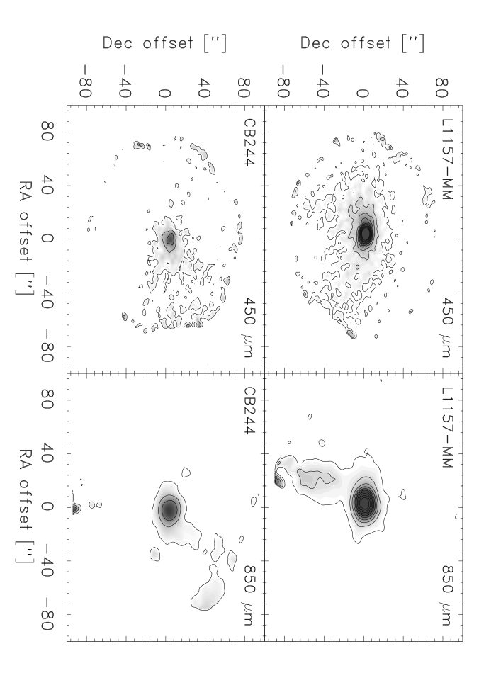
Figure 1: SCUBA images of CB244 and L1157 at 450 and 850 $\mu$m. The contours indicate the intensity corresponding to 2$\sigma$, 4$\sigma$, etc. with $\sigma$ being the RMS noise given for each source and wavelength in Table 3.

2.4 Line data

CO line data were obtained with the JCMT in May and August 2001, the Instituto de Radio Astronomica Milimetrica (IRAM) 30m telescope in November 2001 and the Onsala Space Observatory 20m telescope in March 2002, complementing data from the JCMT archive. Our own observations were performed in beam switching mode using a switch of 180″ in declination - except for the sources in NGC1333, where position switching towards an emission free reference position was used. A more detailed description of the JCMT and the heterodyne receivers can be found on the JCMT homepage. Where archive data were available for one line from several different projects, the data belonging to each observing program were reduced individually and the results compared giving an estimate of the calibration uncertainty of the data of 20%. The integrated line intensities were found by fitting gaussians to the main line. In some cases outflow or secondary components were apparent in the line profiles leading to two gaussian fits. For the C¹⁷O $J=1-0$ and $J=2-1$ lines, the hyperfine splitting were apparent, giving rise to two separate lines for the $J=1-0$ transition separated by about 5 km s^-1, while the $J=2-1$ main hyperfine lines are split by less (0.5 km s^-1) giving rise in some cases to line asymmetries. In these cases the quoted line intensities are the total intensity including all hyperfine lines.

The integrated line data were brought from the antenna temperature scale $T_{\rm A}^{\ast}$ to the main-beam brightness scale $T_{\rm mb}$ by dividing by the main-beam brightness efficiency $\eta_{\rm mb}$ taken to be 0.69 for data obtained using the JCMT A band receivers (210-270 GHz; the $J=2-1$ transitions) and 0.59-0.63 for respectively the old B3i (before December 1996) and new B3 receivers (330-370 GHz; the $J=3-2$ transitions). For the IRAM 30m observations beam efficiencies $B_{\rm eff}$ of 0.74 and 0.54 and forward efficiencies $F_{\rm eff}$ of 0.95 and 0.91 were adopted for respectively the C¹⁷O $J=1-0$ and $J=2-1$ lines, which corresponds to main-beam brightness efficiencies ($\eta_{\rm mb}=B_{\rm eff}/F_{\rm eff}$) of respectively 0.78 and 0.59. For the Onsala 20m telescope $\eta_{\rm mb}=0.43$ was adopted for the C¹⁸O and C¹⁷O $J=1-0$ lines. The relevant beam sizes for the JCMT are 21″ and 14″ at respectively 220 and 330 GHz, for the IRAM 30m, 22″ and 11″ at respectively 112 and 224 GHz and for the Onsala 20m, 33″. The velocity resolution ranged from 0.1–0.3 km s^-1 for the JCMT data and were 0.05 and 0.1 km s^-1 for the observations of respectively the C¹⁷O $J=1-0$ and $J=2-1$ transitions at the IRAM 30m. The line properties are summarized later in Sect. 5.

3 Continuum modelling

3.1 Input

To model the physical properties of the envelopes around these sources the 1D radiative transfer code DUSTY (Ivezić et al., 1999) was used. The dust grain opacities from Ossenkopf & Henning (1994) corresponding to coagulated dust grains with thin ice mantles at a density of $n_{\rm H_{2}}\sim 10^{6}\,{\rm cm}^{-3}$ were adopted. These were found by van der Tak et al. (1999) to be the only dust opacities that could reproduce the “standard” dust-to-gas mass ratio of 1:100 by comparison to C¹⁷O measurements for warm high-mass YSOs where CO is not depleted.

Using a power-law to describe the density leaves five parameters to fit as summarized in Table 4. Not all five parameters are independent, however: the temperature at the inner boundary, $T_{1}$, determines the inner radius of the envelope, $r_{1}$, through the luminosity of the source. If the outer radius of the envelope $r_{2}$ is expected to be constant, $Y=r_{2}/r_{1}$ will depend on the value of $r_{1}$, i.e., $T_{1}$. The results are, however, not expected to depend on $r_{1}$ if it is chosen small enough, since the beam size does not resolve the inner parts anyway. Therefore $T_{1}$ is simply set to 250 K, a reasonable temperature considering the chemistry observed towards these sources. Also the temperature of the central star has to be fixed: a temperature of 5000 K is chosen. This temperature is of course mostly unknown for the embedded sources, but due to the optical thickness of the envelope most of the radiation from the central star is anyway reprocessed by the dust and thus the temperature of the central star does not play a critical role, e.g., in the resulting SED.

Although these parameters may not seem the most straightforward choice, one of the advantages of DUSTY is the scale-free nature allowing the user to run a large sample of models and then compare a number of YSOs to these models just by scaling with distance and luminosity as discussed in Ivezić et al. (1999).

Table 4: Parameters for the DUSTY 1D radiative transfer modelling of the protostellar envelopes.

Param.	Description
Modelled:
$Y$	Ratio of the outer ($r_{2}$) to inner ($r_{1}$) radius
$\tau_{100}$	Optical depth at 100 $\mu$m
$\alpha$	Density power-law exponent
Fixed:
$T_{1}$	Temperature at inner boundary (250 K)
$T_{\star}$	Temperature of star (5000 K)
Literature:
$d$	Distance
$L_{\rm bol}$	Luminosity

3.2 Output

DUSTY provides fluxes at various wavelengths and brightness profiles for the sources, which are compared to the SCUBA data and flux measurements. Given the grid of models the best fit model can then be determined by calculating the $\chi^{2}$-statistics for the SED and brightness profiles at 450 and 850 $\mu$m ($\chi^{2}_{\rm SED}$, $\chi^{2}_{450}$ and $\chi^{2}_{850}$ respectively). In order to fully simulate the observations, the modelled brightness profiles are convolved with the exact beam as obtained from planet observations. Strictly speaking, the outer parts of the brightness profile also depend on the chopping of the telescope. The chopping along one axis does by nature not obey the spherical symmetry, so simulation of the chopping and comparing this with one dimensional modelling will not reflect the observations. Therefore in this analysis only the inner 60″ of the brightness profiles are considered, which (1) should be less sensitive to the typical 120″ chop and (2) is typically above the background emission. For the flux measurements a relative uncertainty of 20% was assumed irrespective of what was given in the original reference, since some authors tend to give only statistical errors and do not include calibration or systematic errors. By assigning a relative uncertainty of 20% to all measurements each point is weighted equal but more weight is given to a given part of the SED if several independent measurements exist around a certain wavelength. Contour plots of the derived $\chi^{2}$ values for L483-mm are presented in Fig. 2, while the actual fits to the brightness profiles and the SED for this source are shown in Fig. 3 and 4.

In determining the best fit model each of the calculated $\chi^{2}$ values are considered individually. The total $\chi^{2}$ obtained by adding the $\chi^{2}_{\rm SED}$, $\chi^{2}_{850}$ and $\chi^{2}_{450}$ does not make sense in a strictly statistical way, since the observations going into these cases are not 100% independent. Another reason for not combining the values of $\chi^{2}_{\rm SED}$, $\chi^{2}_{450}$ and $\chi^{2}_{850}$ into one total $\chi^{2}$ is that the parameters constrained by the SED and brightness profiles are different. For example the brightness profiles provide good constraints on $\alpha$ as seen in a 2D contour ($Y,\alpha$) plot of, e.g., $\chi^{2}_{450}$ in Fig. 2, while these do not depend critically on the value of $\tau_{100}$. The most characteristic feature of the $\chi^{2}$-values for the SEDs on the other hand is the band of possible models in contour plots for ($\alpha,\tau_{100}$), giving an almost one-to-one correspondence for a best fit $\tau_{100}$ for each value $\alpha$.

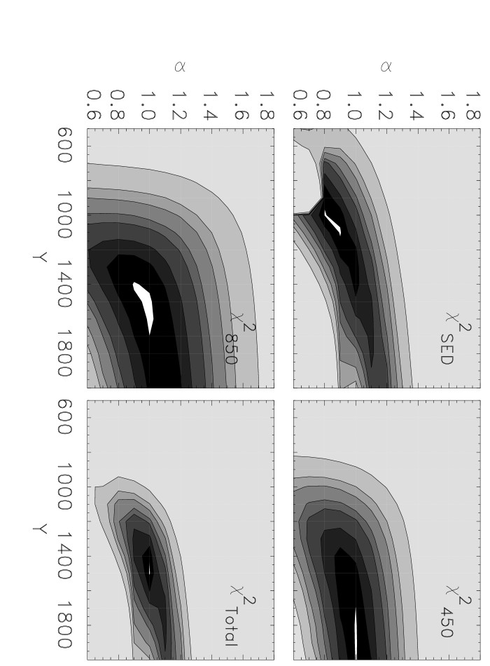
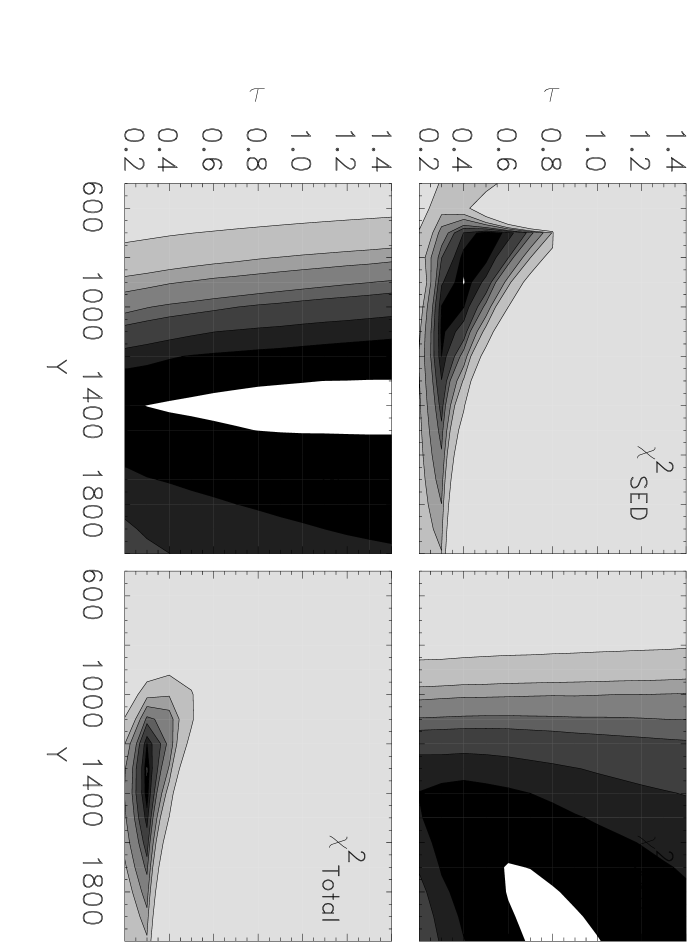
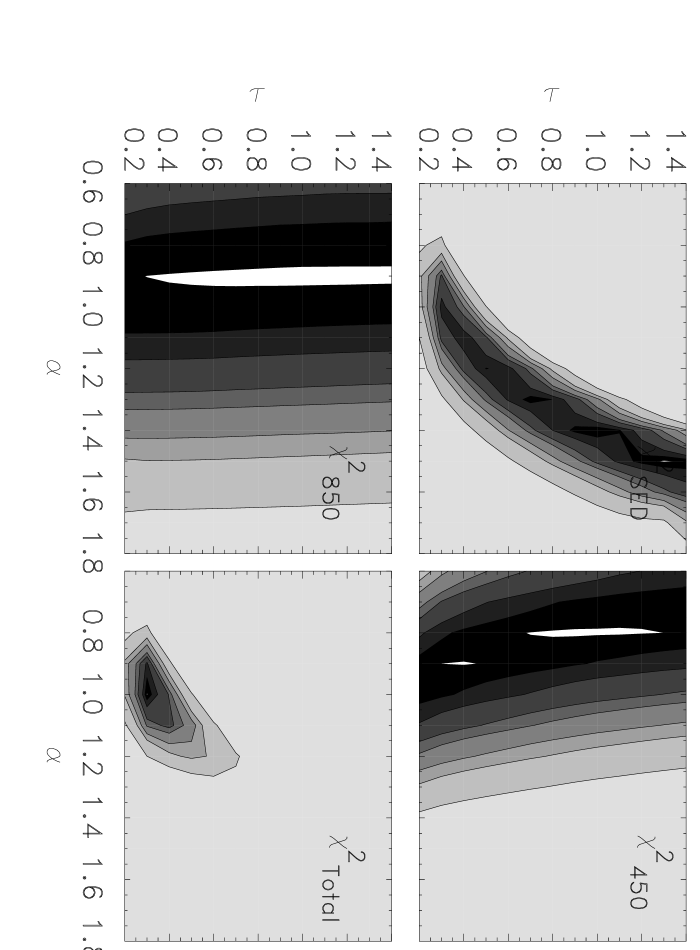
Figure 2: $\chi^{2}$ contour plots for the modelling of L483-mm. In the four upper panels $\tau_{100}$ is fixed at 0.2, in the 4 middle panels $\alpha$ is fixed at 0.9 and while in the 4 lower panels $Y$ is fixed at 1400. The solid (dark) contours indicate the confidence limits corresponding to 1$\sigma$, 2$\sigma$ etc.

These features are actually easily understood: $\chi^{2}_{450}$ and $\chi^{2}_{850}$ are the normalized profiles and should thus not depend directly on the value of $\tau_{100}$. On the other hand since the peaks of the SEDs are typically found at wavelengths longer than 100 $\mu$m, increasing $\tau_{100}$ and thus the flux at this wavelength, require the best-fit SED to shift towards 100 $\mu$m, i.e., with less material in the outer cool parts of the envelope, which can be obtained by a steeper value of $\alpha$. The value of $Y$ is less well constrained, mainly because of its relation to the temperature at the inner radius (and through that the luminosity of the central source). As illustrated in Fig. 2, $Y$ is constrained within a factor 1.5-2.0 at the $2\sigma$ level, but the question is how physical the outer boundary of the envelope is: is a sharp outer boundary expected or rather a soft transition as the density and temperature in the envelope reaches that of the surrounding molecular cloud? In the first case, a clear drop of the observed brightness profile should be seen compared with a model with a (sufficiently) large value of $Y$, e.g., corresponding to an outer temperature of 5–10 K, less than the temperature of a typical molecular cloud. In the other case, however, such a model will be able to trace the brightness profile all the way down to the noise limit. The modelling of the CO lines (see Sect. 5) indicates that significant ambient cloud material is present towards most sources, so the transition from the isolated protostar to the parental cloud is likely to be more complex than described by a single power-law.

The features of the values of $\chi^{2}_{\rm SED}$, $\chi^{2}_{450}$ and $\chi^{2}_{850}$ provide an obvious strategy for selecting the best fit models: first the best fit value of $\alpha$ is selected on the basis of the brightness profiles and second the corresponding value of $\tau_{100}$ is selected from the $\chi^{2}_{\rm SED}$ contour plots. For a few sources there is not 100% overlap between the 450 and 850 $\mu$m brightness profiles and it is not clear which brightness profile is better. The beam at 850 $\mu$m is significantly larger than that at 450 $\mu$m (15″ vs. 9″) and even though the beam is taken into account explicitly, the sensitivity of the 850 $\mu$m data to variations in the density profile must be lower as is seen from Fig. 2. On the other hand, the 450 $\mu$m data generally suffer from higher noise, so especially the weak emission from the envelope, which provides the better constraints on the outer parts of the envelope and thus the power-law exponent, will be more doubtful at this wavelength. The power-law slopes found from modelling the two brightness profiles agree, however, within the uncertainties ($\alpha\sim\pm 0.2$).

Figure 3: The observed brightness profile for L483 at 450 $\mu$m (upper panel) and 850 $\mu$m (lower panel) with the best-fit models overplotted (full line). The dashed line indicates the beam profile used in the modelling.

Figure 4: The spectral energy distribution of L483: the points indicate the data, the line the best-fit model.

3.3 Results

In Table 5, the fitted values of the three parameters for each source are presented and in Table 6 the physical parameters obtained by scaling according to source distance and luminosities are given. As obvious from the $\chi^{2}$ plots in Fig. 2, these parameters have some associated uncertainties. The value of $\alpha$ is determined typically within $\pm 0.2$ leading to a similar uncertainty in $\tau_{100}$ of $\pm 0.2$. The minimum value of $Y$ gives a corresponding minimum value of the outer radius. As discussed above, increasing $Y$ only corresponds to adding more material after the outer boundary, so if $Y$ is large enough to encompass the point where the temperature $T$ reaches 10 K, the radius corresponding to this temperature can be used as a characteristic size of the envelope. The region of the envelopes within this radius corresponds to the inner 40-50″ of the brightness profiles for all the sources. If one would increase the radius further, the typical 120″ chop throw for SCUBA should be taken into account when comparing the brightness profiles from the models with the observations. This could lead to flatter density profiles with $\alpha$ decreased by $\sim 0.2$ (e.g. Motte & André, 2001). Although the models presented here do not extend that far, one should still be aware of the possibility that emission is picked up at the reference position, which would lead to an overestimate of the steepness of the density distribution. The fitted brightness profiles and SEDs for all sources are presented in Fig. 5, 6 and 7.

Table 5: Best fit parameters from DUSTY modelling.

Source	$Y$(a)	$\alpha$	$\tau_{100}$
L1448-I2	1800	1.2	1.1
L1448-C	1600	1.4	0.5
N1333-I2	900	1.8	1.6
N1333-I4A	1000	1.8	6.5
N1333-I4B	1400	1.3	0.9
L1527	2500	0.6	0.1
VLA1623	2400	1.4	0.7
L483	1400	0.9	0.3
L723	2500	1.5	1.0
L1157	600	1.7	3.4
CB244	2600	1.1	0.2
L1489	1200	1.8	0.3
TMR1	2000	1.6	0.1
L1551-I5	1000	1.8	1.1
TMC1A	1700	1.9	1.3
TMC1	2900	1.6	0.2
L1544	2800	0.1	0.1
L1689B	3000	0.1	0.2

Notes: ^(a)Value corresponding to $r_{2}/r_{1}$ in Table 6.

Table 6: Result of DUSTY modelling - derived physical parameters.

Source	$r_{1}$	$r_{2}$	$r_{\rm 10K}$	$N_{\rm H_{2},10K}$	$M_{\rm 10K}$	$n(r_{1})$	$n_{1000{\rm AU}}$	$n_{10{\rm K}}$
	(AU)	(AU)	(AU)	(cm-2)	(M⊙)	(cm-3)	(cm-3)	(cm-3)
L1448-I2	7.4	$1.3\times 10^{4}$	$4.5\times 10^{3}$	$3.5\times 10^{23}$	1.5	$8.8\times 10^{8}$	$2.5\times 10^{6}$	$4.0\times 10^{5}$
L1448-C	9.0	$1.5\times 10^{4}$	$8.1\times 10^{3}$	$1.7\times 10^{23}$	0.93	$5.4\times 10^{8}$	$7.5\times 10^{5}$	$4.0\times 10^{4}$
N1333-I2	23.4	$2.1\times 10^{4}$	$1.2\times 10^{4}$	$5.5\times 10^{23}$	1.7	$1.3\times 10^{9}$	$1.5\times 10^{6}$	$1.7\times 10^{4}$
N1333-I4A	23.9	$2.4\times 10^{4}$	$4.7\times 10^{3}$	$2.2\times 10^{24}$	2.3	$5.0\times 10^{9}$	$6.3\times 10^{6}$	$3.8\times 10^{5}$
N1333-I4B	10.6	$1.5\times 10^{4}$	$7.0\times 10^{3}$	$3.0\times 10^{23}$	2.0	$6.7\times 10^{8}$	$1.8\times 10^{6}$	$1.4\times 10^{5}$
L1527	4.2	$1.1\times 10^{4}$	$6.3\times 10^{3}$	$2.8\times 10^{22}$	0.91	$9.9\times 10^{6}$	$3.8\times 10^{5}$	$1.2\times 10^{5}$
VLA1623	4.3	$1.0\times 10^{4}$	$3.3\times 10^{3}$	$2.3\times 10^{23}$	0.22	$1.6\times 10^{9}$	$7.7\times 10^{5}$	$1.5\times 10^{5}$
L483	21.5	$3.2\times 10^{4}$	$7.8\times 10^{3}$	$9.3\times 10^{23}$	1.1	$2.7\times 10^{9}$	$1.7\times 10^{6}$	$3.4\times 10^{4}$
L723	8.2	$2.1\times 10^{4}$	$5.4\times 10^{3}$	$3.4\times 10^{23}$	0.62	$1.4\times 10^{9}$	$1.1\times 10^{6}$	$8.6\times 10^{4}$
L1157	17.9	$1.1\times 10^{4}$	$5.4\times 10^{3}$	$1.2\times 10^{24}$	1.6	$3.1\times 10^{9}$	$3.3\times 10^{6}$	$1.9\times 10^{5}$
CB244	3.3	$8.7\times 10^{3}$	$4.3\times 10^{3}$	$6.5\times 10^{22}$	0.28	$2.5\times 10^{8}$	$4.8\times 10^{5}$	$9.7\times 10^{4}$
L1489	7.8	$9.4\times 10^{3}$	$9.2\times 10^{3}$	$1.0\times 10^{23}$	0.097	$7.1\times 10^{8}$	$1.2\times 10^{5}$	$2.1\times 10^{3}$
TMR1	6.7	$1.3\times 10^{4}$	$1.2\times 10^{4}$	$3.5\times 10^{22}$	0.12	$2.1\times 10^{8}$	$6.9\times 10^{4}$	$1.3\times 10^{3}$
L1551-I5	24.8	$2.5\times 10^{4}$	$1.6\times 10^{4}$	$3.8\times 10^{23}$	1.7	$8.2\times 10^{8}$	$1.1\times 10^{6}$	$7.2\times 10^{3}$
TMC1A	8.4	$1.4\times 10^{4}$	$4.8\times 10^{3}$	$4.5\times 10^{23}$	0.13	$3.2\times 10^{9}$	$3.7\times 10^{5}$	$1.8\times 10^{4}$
TMC1	3.1	$9.0\times 10^{3}$	$4.3\times 10^{3}$	$6.9\times 10^{22}$	0.034	$9.0\times 10^{8}$	$8.8\times 10^{4}$	$8.5\times 10^{3}$
L1544	3.0	$8.3\times 10^{3}$	$4.0\times 10^{3}$	$1.8\times 10^{22}$	0.41	$5.5\times 10^{5}$	$3.1\times 10^{5}$	$2.7\times 10^{5}$
L1689B	1.3	$4.0\times 10^{3}$	$1.5\times 10^{3}$	$2.9\times 10^{22}$	0.096	$2.3\times 10^{6}$	$1.2\times 10^{6}$	$1.1\times 10^{6}$

Figure 5: Composite showing the brightness profiles of the sources overplotted with the best fit model at 450 $\mu$m. The dashed line indicate the beam profile.

Figure 6: As in Fig. 5 but for the 850 $\mu$m data.

Figure 7: Composite showing the SEDs of each source overplotted with the SED from the best fit model. The individual SEDs are based on literature searches, with the main references being Shirley et al. (2000) (class 0 objects and pre-stellar cores), Chandler & Richer (2000) (NGC1333-I2), Sandell et al. (1991) (NGC1333-I4A,B; 350 and 800 $\mu$m), IRAS Faint Source Catalog (TMR1, L1489) and 1.3 mm fluxes from Motte & André (2001) for sources included in their sample.

The derived power-law indices are for most sources in agreement with the predictions from the inside-out collapse model of $\alpha=1.5-2.0$. A few YSOs (esp. L1527, L483, CB244 and L1448-I2) have density distributions that are flatter, but as argued in Sect. 4.2, this can be explained by the fact that these sources seem to have significant departures from spherical symmetry. Apart from these sources, there is no apparent distinction between the class 0 and class I sources in the sample as shown in the plot of power-law slope versus bolometric temperature in the upper panel of Fig. 8. There is, however, a significant difference in the masses derived for these types of objects, with the class 0 objects having significantly more massive envelopes (lower panel of Fig. 8). This is to be expected since the bolometric temperature measures the redness (or coolness) of the SED, i.e., the amount of envelope material. Finally, there is no dependence on either mass or power-law slope with distance, which strengthens the validity of the derived parameters.

Figure 8: The slope of the density distribution (upper panel) and the mass within the 10 K radius (lower panel) vs. the bolometric temperature of the sources. Class 0 objects are marked by “$\blacklozenge$”, class I objects by “$\blacktriangle$” and pre-stellar cores by “$\blacksquare$”. VLA1623 and IRAS 16293-2422 have been singled out with respectively “$\bullet$” and “$\bigstar$”. The mass of the pre-stellar cores in the lower panel is the mass of the Bonnor-Ebert sphere adopted for the line modelling.

3.4 Individual sources

For some of the sources the derived results are uncertain for various reasons, e.g., the interpretation of their surrounding environment. These cases together with other interesting properties of the sources are briefly discussed below. The failure of our power-law approach to describe the pre-stellar cores will be further discussed in Sect. 4.3.

N1333-I2,-I4:

A major factor of uncertainty in the determination of the parameters for the sources associated with the reflection nebula NGC1333 is the distance of these sources. Values ranging from 220 pc (Černis, 1990) to 350 pc (Herbig & Jones, 1983) have been suggested. The latter determination of the distance assumes that NGC 1333 (and the associated dark cloud L1450) is part of the Perseus OB2 association, which recent estimates place at $318\pm 27$ pc (de Zeeuw et al., 1999). The first value is a more direct estimate based on the extinction towards the cloud. N1333-I2 can be modelled using either distance - but the 10 K radius becomes rather large, i.e., 19000 AU in the case of an assumed distance of 350 pc, while the distance of 220 pc leads to a radius of 11000 AU that is more consistent with those of the other sources.

N1333-I4 is one of the best-studied low-mass protostellar systems, both with respect to the molecular content (Blake et al., 1995) and in interferometric continuum studies (Looney et al., 2000). On the largest scales the entire system is seen to be embedded in a single envelope, but going to progressively smaller scales shows that both N1333-I4A and N1333-I4B are multiple in nature (Looney et al., 2000). The small separation between the two sources can cause problems when interpreting the emission from the envelopes of each of the sources. On the other hand the small scale binary components of N1333-I4A and N1333-I4B each should be embedded in common envelopes and can at most introduce a departure from the spherical symmetry.

L1448-C, -I2:

The L1448 cloud reveals a complex of 4 or more class 0 objects with L1448-C (or L1448-mm) and its powerful outflow together with the binary protostar L1448-N being well studied (e.g., Barsony et al., 1998). Also the recently identified L1448-I2 (O’Linger et al., 1999) shows typical protostellar properties. The dark cloud L1448 itself is a member of the Perseus molecular cloud complex, for which we adopt a distance of 220 pc (see above). Note, however, that Černis (1990) mentions the possibility of a distance gradient across the cloud complex so that larger distances may be appropriate for the L1448 objects.

VLA 1623:

As the first “identified” class 0 object, VLA 1623 is often discussed as a prototype class 0 object. It is, however, not well suited for discussions of the properties of these objects because of its location close to a number of submillimeter cores (e.g., Wilson et al., 1999). This makes it hard to extract and model the properties of this source and might explain why it has been claimed to have a very shallow density profile of $\rho\propto r^{-0.5}$ (André et al., 1993) or a constant density outer envelope (Jayawardhana et al., 2001). If the emission in the three quadrants towards the other submillimeter cores is blocked out when creating the brightness profiles it is found that VLA 1623 can be modelled with an almost “standard” density profile with $\alpha=1.4$, although with rather large uncertainties.

L1527:

L1527 is remarkable for its rather flat envelope profile with $\alpha\approx 0.6$. It was one of the sources for which Chandler & Richer (2000) estimated the relative contribution of the disk and envelope to the total flux at 450 and 850 $\mu$m and found that the envelope contributes by more than 85%, which justifies our use of the images at these wavelengths to constrain the envelope. On the other hand, Hogerheijde et al. (1997) estimate the disk contribution at 1.1 mm in a 19″ beam to be between 30 and 75% of the continuum emission ($\approx$ 50% for L1527) for a sample of mainly class I objects, so it is evident that possible disk emission is a factor of uncertainty in the envelope modelling. Disk emission would contribute to the fluxes of the innermost points on the brightness profiles and so lead to a steeper density profile.

L723-mm:

The most characteristic feature about L723-mm is the quadrupolar outflow originating in the central source, which has lead to the suggestion that the central star is a binary (Girart et al., 1997).

L483-mm:

L483-mm is a good example of a central source with an asymmetry yet providing an excellent fit to the brightness profile with the simple power-law (see discussion in Sect. 4.2). The source seems to be located in a flattened filament showing up clearly in the SCUBA maps (e.g., Shirley et al., 2000) and integrated NH₃ emission (Fuller & Wootten, 2000).

L1157-mm:

L1157-mm is not as well known for the protostellar source itself as for its bipolar outflow, where a large enhancement of chemical species like CH₃OH, HCN and H₂CO is seen (e.g., Bachiller & Pérez Gutiérrez, 1997). As a result, the SED of the protostar itself is rather poorly determined. Our images in Fig. 3 show a source slightly extended in the east-west direction and with a second object showing up south of the source in the 850 $\mu$m data. Recently Chini et al. (2001) reported a similar observation of the source and added that the southern feature is also seen in the 1.3 mm data in the direction of the CO outflow from L1157, suggesting an interaction between the outflowing gas and the circumstellar dust.

CB244:

CB244 is the only protostar of our sample not included in the table of André et al. (2000). Launhardt et al. (1997) found that this relatively isolated globule indeed has a high submillimeter flux, $L_{\rm bol}/L_{\rm submm}\geq 2\%$ qualifying it as a class 0 object. It is, however, probably close to the boundary between the class 0 and I stages: Saraceno et al. (1996) found that it falls in the area of the class I objects in a $L_{\rm bol}$ vs. $F_{\rm mm}$ diagram.

L1489:

Of the two class I sources in our main sample, L1489 has recently drawn attention with the suggestion that the central star is surrounded by a disk-like structure rather than the “usual” envelope for class 0/I objects (Hogerheijde & Sandell, 2000; Hogerheijde, 2001). Hogerheijde & Sandell examined the SCUBA images of this source in comparison with the line emission with the purpose of testing the different models for the envelope structure - especially the Shu (1977) infall model. They found that L1489 could not be fitted in the inside-out collapse scenario, if both the SCUBA images and spectroscopic data are modelled simultaneously. Instead they suggested that L1489 is an object undergoing a transition from the class I to II stages, revealing a 2000 AU disk, whose velocity structure is revealed through high resolution HCO⁺ interferometer data (Hogerheijde, 2001). That we actually can fit the SCUBA data is neither proving nor disproving this result. Hogerheijde & Sandell in fact remark that it is possible to fit the continuum data alone, but that this would correspond to an unrealistic high age of this source. The modelling of L1489 is slightly complicated by a nearby submillimeter condensation - presumably a pre-stellar core, which has to be blocked out leading to an increase in the uncertainty for the fitting of the brightness profile.

TMR1:

This is a more standard class I object showing a bipolar nebulosity in the infrared corresponding to the outflow cavities of the envelope (Hogerheijde et al., 1998).

4 Discussion and comparison

4.1 Power law or not?

The first simplistic assumption in the above modelling is (as in other recent works, e.g., Shirley et al. (2000); Chandler & Richer (2000); Motte & André (2001)) that the density distribution can be described by a single power law. This is not in agreement with even the simplest infall model, but given the observed brightness profiles of the protostars it is tempting to just approximate the density distribution with a single power law. As an example Shirley et al. (2000), used this approach citing the results of Adams (1991): if the density distribution can be described by a power-law and the beam can be approximated by a gaussian then the outcoming brightness profiles will also be a power-law, so a power-law fit to the outer parts of the brightness profile will directly reflect the density distribution. This approach is, however, subject to noise in the data and the parts of the brightness profile chosen to be considered. On the other hand, our 1D modelling clearly shows that the data do not warrant more complicated fits and that the power-law adequately describes the profiles of the sources. Modelling of the detailed line profiles will require more sophisticated infall models, since signatures for infall exist for around half of the class 0 sources in the sample (André et al., 2000). However, Schöier et al. (2002) show that for the case of IRAS 16293-2422, adopting the infall model of Shu (1977) does not improve the quality of the fit to the continuum data.

Chandler & Richer (2000) assumed that the envelopes were optically thin. In this case, the temperature profile can be shown to be a simple power-law as well and Chandler & Richer subsequently derived analytical models which could be fitted directly to the SCUBA data. For the sources included in both samples the derived power-law indices agree within the uncertainties. However, as illustrated in Fig. 9, the optically thin assumption for the temperature distribution is not valid in the inner parts of the envelope, especially of the more massive class 0 sources, so actual radiative transfer modelling is needed to establish the temperature profile, crucial for calculations of the molecular excitation and chemical modelling.

Disk emission can contribute to the fluxes of the innermost points on the brightness profiles and thus lead to a steeper density profile. This is likely to be more important in the sources with the less massive envelope, i.e. class I objects. In tests where the fluxes within the innermost 15″ of the brightness profiles are reduced by 50%, the best fit values of $\alpha$ are reduced by 0.1–0.2. This is comparable to the uncertainties in the derived value of $\alpha$, but can introduce a systematic error.

It is interesting to note that there is no clear trend in the slope of the density profile with type of object. In the framework of the inside-out collapse model, one would expect a flattening of the density profiles, approaching 1.5 as the entire envelope undergoes the collapse. This is not seen in the data - actually the average density profile for the class I objects is slightly steeper than for the class 0 objects. On the other hand, the suggestion of an outer envelope with a flat density distribution and a significant fraction of material as suggested by Jayawardhana et al. (2001) can also not be confirmed by this modelling. As seen from the fits in Fig. 5 and 6 the brightness profiles only suggest departures from the single power-law fits in the outer regions in a few cases, so if such a component is present, it is not traced directly by the SCUBA maps. The slightly flatter density profiles for the class 0 objects could be a manifestation of such an outer component - but the density distributions of the sources in this sample are typically much steeper (i.e. $\rho\propto r^{-3/2}$) than those modelled by Jayawardhana et al. ($\rho\propto r^{-1/2}$).

Figure 9: The temperature profiles for four selected sources with temperature profiles calculated in the Rayleigh-Jeans limit for the optically thin assumption overplotted for different dust opacity laws, $\kappa_{\nu}\propto\nu^{\beta}$. The dashed line corresponds to $\beta=1$ and the dash-dotted line to $\beta=2$.

4.2 Geometrical effects

As mentioned above, it was assumed in the modelling that the sources are spherical symmetric. This may not be entirely correct considering the structure of YSOs, which may be rotating and are permeated by magnetic fields leading to polar flattening (Terebey et al., 1984; Galli & Shu, 1993) and which are definitely associated with molecular outflows and jets (Bachiller & Tafalla, 1999; Richer et al., 2000). One problem in this discussion is the exact shape of the error beam of SCUBA. Typically an error lobe pickup of 15% in the 850 $\mu$m images and 45% in the 450 $\mu$m maps is estimated. This error beam is not completely spherically symmetric, but is also not well-established, so in fact 1D modelling may be the best that can be done using the SCUBA data.

Myers et al. (1998) investigated the results of departure from spherical symmetry of an envelope when calculating the bolometric temperature of YSOs seen under various inclination angles. With a cavity in the pole region, roughly corresponding to the effect of a bipolar outflow, they found that the bolometric temperature could increase by a factor 1.3–2.5 for a typical opening angle of 25°. A similar line of thought can be applied to our modelling: departure from spherical symmetry by having a thinner polar region will affect the determination of the SED - a source viewed more pole-on will see warmer material which leads to an SED shifted towards shorter wavelengths and accordingly a lower value of $\tau_{100}$. Myers et al. also argued that the effect on a statistical sample would be rather small, e.g., compared to differences in optical depth, but for studies of individual sources like in our case, this effect might be of importance.

The brightness profile will also change in the aspherical case. In the case of a source viewed edge-on this would result in elliptically shaped SCUBA images with the 850 $\mu$m data showing a more elongated structure since the smaller optical depths material in the polar regions would reveal material being warmer and thus having stronger emission at 450 $\mu$m, compensating for the lack of material in these images. If we consider the case where the source is viewed entirely pole-on, the image would still appear circular, but the brightness profiles would show a steeper increase towards the center in the 450 $\mu$m data (closer to the spherical case) than the 850 $\mu$m data for the same reasons as mentioned above.

The good fits to the brightness profiles given the often non-circular nature of the SCUBA images is expected based on the mathematical nature of power-law profiles. Consider as an example a 2D image of a source described by:

$$I=I_{0}\,r^{-f(\theta)}$$ (1)

where $f(\theta)$ is a function describing the variation of the slope of the brightness profiles extracted in rays along different directions away from the center position. In the case of a source with a simple density profile $\rho\propto r^{-p}$ Adams (1991) showed that such sources will also give images with power-law brightness distributions corresponding to the case where $f(\theta)={\rm const}$. As a somewhat simplistic case, assume that $f(\theta)$ is a step function with a power-law slope $p_{1}$ in $\theta\in[0,\pi[$ and a $p_{2}$ in $\theta\in[\pi,2\pi[$. In this case determination of the power-law slope will be dominated by the flattest of the two slopes: the azimuthal averaged brightness profile will be

$$\langle I\rangle_{\theta}\propto r^{-p_{1}}+r^{-p_{2}}$$ (2)

and due to the power-law decline the term corresponding to the shallower slope will dominate the average, especially at the larger radii. This has two effects: first the distribution of power-law “rays” must be very strongly varying in order not to result in a power-law average, and second, the density profile for asymmetric sources will be flattened compared to more spherical sources.

As a test, brightness profiles were extracted in angles covering respectively the flattest and steepest direction of L483 and L1527. Modelling the so-derived brightness profiles gives best-fit density profiles of 0.9 and 1.2, compared to the 0.9 derived as the average over the entire image for L483, and 0.6 and 0.8 for L1527 compared to 0.6 from the entire image. Thus, the brightness profile and the derived density profile might indeed be flattened by the asymmetry and could account for the somewhat flatter profiles found towards some sources. The discrepancies between the profiles along different directions are, however, not much larger than the uncertainties in the derived power-law slope, so these sources could have intrinsic flatter density distributions instead; with the present quality of the data both interpretations are possible.

4.3 Pre-stellar cores

The modelling of the pre-stellar cores is more complicated than that of the class 0 and I sources, since it is not clear whether the cores are undergoing gravitational collapse, or are centrally condensed and/or are gravitationally bound. In the case of thermally supported gravitationally bound cores, the solution for the density profile is the Bonnor-Ebert sphere (Ebert, 1955; Bonnor, 1956). Recently Evans et al. (2001) modelled three pre-stellar cores (including L1689B and L1544 in our sample) and found that they could be well fitted by Bonnor-Ebert spheres. Evans et al. also found that the denser cores, L1689B and L1544, were those showing spectroscopic signs of contraction thus suggesting an evolutionary sequence with L1544 as the pre-stellar cores closest to the collapse phase. This is supported as well by millimeter observations of this core which show a dense inner region (Tafalla et al., 1998; Ward-Thompson et al., 1999).

Evans et al. also discussed the properties of non-isothermal models and found that the quality of the fit to the data is similar to the isothermal case. Ward-Thompson et al. (2002) examined ISOPHOT 200 $\mu$m data for a sample of pre-stellar cores (including L1689B and L1544) and found that none of the cores had a central peak in temperature and that they could all be interpreted as being isothermal or having a temperature gradient with a cold center as result of external heating by the interstellar radiation field. Zucconi et al. (2001) derived analytical formulae for the dust temperature distributions in pre-stellar cores showing that these cores should have temperatures varying from 8 K in the center to around 15 K at the boundary. These equations will be useful for more detailed modelling of the continuum and line data, but for the present purpose the isothermal models are sufficient.

Modelling the pre-stellar cores using our method is not possible as is illustrated by the best fits for the pre-stellar cores shown in Fig. 5-7. Given the observational evidence that these cores do not have central source of heating, what is implicitly assumed in the DUSTY modelling, it is on the other hand comforting that our method indeed distinguishes between these pre-stellar cores and the class 0/I sources and that the obtained fits to the brightness profiles of the latter sources are not just the results of, e.g., the convolution of the “real” brightness profiles with the SCUBA beam.

For modelling of sources without central heating Evans et al. note that their modelling does not rule out a power-law envelope density distribution for L1544, as opposed to, e.g., the case for L1689B: this would imply an evolutionary trend of the pre-stellar cores having a Bonnor-Ebert density distribution, which would then evolve towards a power-law density distribution with an increasing slope as the collapse progresses. In the modelling of spectral line data for the pre-stellar cores we adopt an isothermal Bonnor-Ebert sphere with $n_{c}\sim 10^{6}$ for both L1689B and L1544 as this was the best fitted isothermal model in the work of Evans et al. (2001).

5 Monte Carlo modelling of CO lines

5.1 Method

One main goal of our work is to use the derived physical models as input for modelling the chemical abundances of the various molecules in the envelopes. To demonstrate this approach, modelling of the first few molecules, C¹⁸O and C¹⁷O, is presented here. This modelling also serves as a test of the trustworthiness of the physical models: is it possible to reproduce realistic abundances for the modelled molecules?

The 1D Monte Carlo code developed by Hogerheijde & van der Tak (2000) is used together with the revised collisional rate coefficients from Flower (2001), and a constant fractional abundance over the entire range of the envelope is assumed as a first approximation. Furthermore the dust and gas temperatures are assumed identical over the entire envelope and any systematic velocity field is neglected. In the outer parts of the envelopes, the coupling between gas and dust may break down (e.g. Ceccarelli et al., 1996; Doty & Neufeld, 1997) leading to differences between gas and dust temperatures of up to a factor of 2.

With the given physical model and assumed molecular properties, there are two free parameters which can be adjusted by minimizing $\chi^{2}$ to model the line profiles for each molecular transition: the fractional abundance [X/H₂] and the turbulent line width $V_{\rm D}$. Since emission from the ambient molecular cloud might contribute to the lower lying 1–0 transitions, the derived abundances are based only on fits to the 2–1 and 3–2 lines. The observed and modelled line intensities are summarized in Tables 7-10, whereas the parameters for the best fit models are given in Table 11. While a turbulent line width of $0.5-1.0$ km s^-1 is needed for most sources to fit the actual line profile, the modelled line strengths are only weakly dependent on this parameter compared to the fractional abundance. For example, for L723 one derives C¹⁸O abundances between $3.8\times 10^{-8}$ and $4.0\times 10^{-8}$ from respectively $V_{\rm D}=1.1$ km s^-1 (FWHM $\simeq 1.9$ km s^-1) to $V_{\rm D}=0.7$ (FWHM $\simeq 1.2$ km s^-1), which should be compared to the [C¹⁸O/H₂]$=3.9\times 10^{-8}$ and $V_{\rm D}=0.8$ km s^-1 (FWHM $\simeq 1.4$ km s^-1) quoted in Table 11. The C¹⁸O and C¹⁷O spectra for L723 and N1333-I2 with the best fit models overplotted are shown in Fig. 10. The revised collisional rate coefficients from Flower (2001) adopted for this modelling typically change the derived abundances by less than 5% compared to results obtained from simulations with previously published molecular data. The relative intensities of the various transitions and so the quality of the fits remain the same.

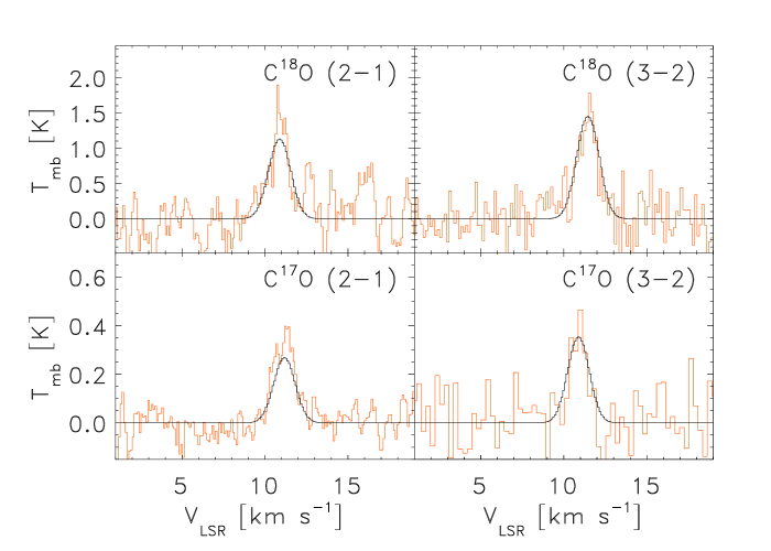
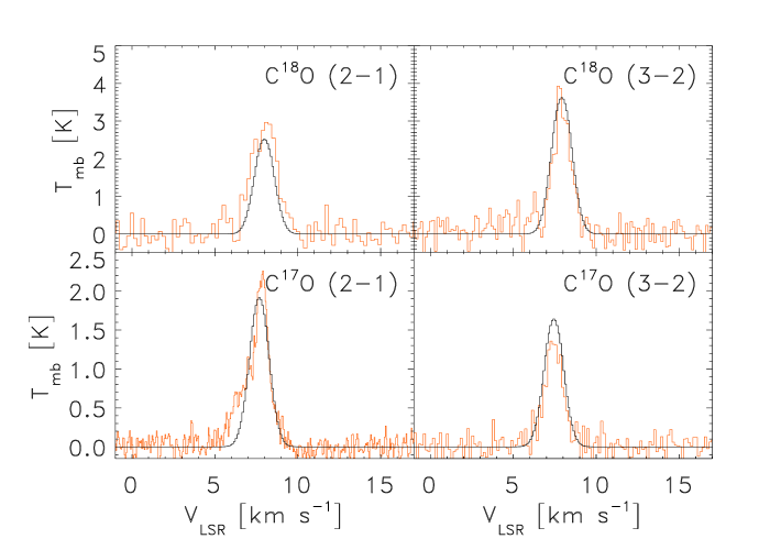
Figure 10: The C¹⁸O and C¹⁷O spectra for L723 (upper four panels) and N1333-I2 (lower four panels) overplotted with the best fit models from the Monte Carlo modelling.

As it is evident from Tables 7-10, the 2–1 and 3–2 lines can be well modelled using the above approach, while the 1–0 lines are significantly underestimated from the modelling, especially in the larger Onsala 20m beam. This indicates that the molecular cloud material may contribute significantly to the observations or that the assumed outer radius is too small. The importance of the latter effect was tested by increasing the outer radius of up to a factor 2.5 for a few sources and it was found that while the 1–0 and 2–1 line intensities could increase in some cases by up to a factor of 2, the 3–2 line intensities varied by less than 10%, illustrating that the 3–2 line mainly trace the warmer ($\geq$ 30 K) envelope material.

The importance of the size of the inner radius was tested as well. For L723 fixing the inner radius at 50 AU rather than 8 AU increases the best fit abundance by $\sim$ 5% to [C¹⁸O/H₂]$=4.1\times 10^{-8}$ without changing the quality of the fit significantly (drop in $\chi^{2}$ of $\sim$ 0.1). This is also found for other sources in the sample and simply illustrates that increasing the inner radius corresponds to a (small) decrease in mass of the envelope, so that a higher CO abundance is required to give the same CO intensities. Yet, it is good to keep in mind that the inner radius of the envelope may be different, and even though its value does not change the results for CO, it might for other molecules, e.g., CH₃OH and H₂CO, which trace the inner warm and dense region of the envelope.

Table 7: The observed C¹⁸O and C¹⁷O lines from the JCMT observations compared to the modelled intensities.

Source	$\Delta V_{\rm av}$	$V_{\rm LSR}$	(2–1)		(3–2)
	(km s-1)(a)	(km s-1)	Obs(b)	Mod(c)	Obs(b)	Mod(c)
C18O
L1448-I2	0.7	4.5	$\ldots$	1.6	1.9$\ast$	1.9
L1448-C	1.2	5.3	4.3	3.3	3.3$\ast$	3.9
N1333-I2	1.4	7.7	5.8	3.9	4.7$\ast$	5.7
N1333-I4A	1.7	7.2	5.5	5.4	$\ldots$	7.1
N1333-I4B	2.1	7.4	4.3	3.8	4.0$\ast$	4.4
L1527	0.7	5.9	4.4	2.9	2.3	2.7
VLA1623	1.0	3.5	12.1:	12.1	12.6:	12.6
L483	1.0	5.2	4.1	3.7	3.6	3.8
L723	1.6	11.2	2.2	1.9	2.2$\ast$	2.4
L1157	0.8	2.6	1.7	1.2	1.4	1.7
CB244	1.1	4.4	3.3	2.9	2.9	3.1
L1489	2.1	7.2	2.7	2.6	3.8	3.9
TMR1	1.5	6.3	4.0	3.3	3.8	4.3
L1551-I5	2.1	7.2	7.1	6.1	8.7	9.7
TMC1A	1.5	6.6	1.3	1.5	2.8	2.3
TMC1	1.5	5.2	2.3	2.7	4.3	3.2
L1544	0.3	7.6	$\ldots$	0.55	0.30	0.30
L1689B	0.6	3.6	3.6	3.3	1.8	1.9
C17O
L1448-I2	0.9	4.0	$\ldots$	0.61	0.71$\ast$	0.72
L1448-C	1.4	5.0	1.5	1.4	1.7$\ast$	1.7
N1333-I2	1.3	7.5	$\ldots$	1.4	1.8$\ast$	2.1
N1333-I4A	1.3	6.7	$\ldots$	1.1	1.4$\ast$	1.6
N1333-I4B	1.4	6.8	$\ldots$	0.9	$\ldots$	1.1
L1527	0.5	6.0	1.9	1.7	1.3	1.6
VLA1623	0.8	3.7	$\ldots$	3.8	4.6:$\ast$	4.5
L483	0.8	5.3	1.5	1.3	1.2$\ast$	1.3
L723	1.3	11.0	0.59	0.43	0.49$\ast$	0.57
L1157	1.0	2.7	0.51	0.47	0.65$\ast$	0.69
CB244	1.0	4.2	0.94	0.68	0.60$\ast$	0.73
L1489	3.0	7.3	$\ldots$	0.56	0.86$\ast$	0.88
TMR1	1.6	6.0	$\ldots$	0.69	0.84$\ast$	0.94
L1551-I5	2.1	7.2	2.2	1.8	2.6	3.1
TMC1A	1.5	6.6	$\ldots$	0.45	$\ldots$	0.73
TMC1	1.5	5.2	$\ldots$	0.83	$\ldots$	1.0
L1544	0.6	7.5	0.26	0.26	$\ast$(d)	0.14
L1689B	0.6	3.7	0.71	0.85	0.59$\ast$	0.44

Notes: ^(a)The width (FWHM) of the lines. ^(b)Observed intensities, $\int T_{\rm mb}$ d$V$ in K km s^-1: our own observations are marked with ’$\ast$’ and lines where double gaussians were fitted and the broadest component subtracted marked with ’:’. ^(c)Modelled intensities in K km s^-1. ^(d)C¹⁷O 3–2 not detected towards L1544 in integrations corresponding to an RMS of 0.1 K ($T_{A}^{\ast}$).

Table 8: As in Table 7 but for the IRAM 30m observations - all from November 2001 observing run.

Source	C17O 1–0		C17O 2–1
	Obs	Mod	Obs	Mod
L1448-C	0.58	0.71	2.2	2.3
N1333-I2	1.1	0.61	3.4	2.5
N1333-I4A	0.99	0.54	2.9	2.3
N1333-I4B	0.73	0.47	1.8	1.5
L1527	1.1	0.90	2.4	2.0
L1489	0.37	0.27	1.1	1.1
TMR1	0.69	0.37	1.4	1.3

Notes: The intensities are the total observed intensity summed over the hyperfine-structure lines.

Table 9: As in Table 7 and 8 for the Onsala 20m observations - all from March 2002 observing run.

Source	C18O 1–0		C17O 1–0
	Obs	Mod	Obs	Mod
L1448-I2	3.2	0.5	1.1	0.2
L1448-C	3.6	1.3	$\ldots$	0.5
N1333-I2	5.6	1.4	1.6	0.5
N1333-I4A	4.2	1.9	$\ldots$	0.4
N1333-I4B	4.1	1.5	$\ldots$	0.4
L1527	2.4	1.5	$\ldots$	0.8
L483	3.8	1.7	2.2	0.6
L723	1.6	0.6	0.3	0.1
L1157	1.3	0.3	0.2	0.1
CB244	1.9	1.1	$\ldots$	0.2
L1489	1.7	1.0	$\ldots$	0.2
TMR1	1.7	1.5	$\ldots$	0.3
L1544	1.7	0.3	0.6	0.2

Notes: ^(a)The intensities are the total observed intensity summed over the hyperfine-structure lines.

Table 10: As Tables 7–9 for CSO measurements from the literature.

Source	C18O 3–2(a)		C17O 3–2(a)
	Obs	Mod	Obs	Mod
N1333-I4A	4.9	4.9	1.0	1.0
N1333-I4B	3.3	3.3	0.80	0.80
	C17O 2–1(b)
TMC1A	0.28	0.27
TMC1	0.53	0.51

Notes: ^(a)From Blake et al. (1995), half-power beam width of 20″. ^(b)From Ladd et al. (1998), half-power beam width of 33″.

5.2 CO abundances

The fitted abundances are summarized in Table 11 and plotted against the envelope mass of each individual source in Fig. 11. As can be seen from the values of the reduced $\chi^{2}$ for the fit to the data for each isotope, the model reproduces the excitation of the individual species. Even in the “worst case” of N1333-I2, the lines do indeed seem to be well-fitted by the model (see Fig. 10). One source, VLA1623 shows a remarkably high ratio between the C¹⁸O and C¹⁷O abundances of 12.4 and high C¹⁸O and C¹⁷O abundances in comparison to the rest of the class 0 sources. Given the location of VLA 1623 close to a dense ridge of material and the associated uncertainties in the physical models of this source, it may reflect problems in the model rather than being a real property of the source. For the rest of the sources, the ratio between the C¹⁸O and C¹⁷O abundances is found to be $3.9\pm 1.3$ in agreement with the expected value from, e.g., the local interstellar medium of 3.65 (Penzias, 1981; Wilson & Rood, 1994) - another sign that the model reproduces the physical structure of the envelopes and that no systematic calibration errors are introduced by using data from the various telescopes and receivers.

It is evident that the class 0 objects (except VLA 1623) and pre-stellar cores show a high degree of depletion compared to the expected abundances of [C¹⁸O/H₂] of $1.7\times 10^{-7}$ from nearby dark clouds (Frerking et al., 1982) and [C¹⁷O/H₂] of $4.7\times 10^{-8}$ assuming ¹⁸O:¹⁷O of 3.65. With this isotope ratio and assuming ¹⁶O:¹⁸O equal to 540 (Wilson & Rood, 1994), the average abundance for the class I sources is $(1.1\pm 0.9)\times 10^{-4}$ and for the class 0 sources and pre-stellar cores $(2.0\pm 1.3)\times 10^{-5}$. The error bars illustrate the source to source variations and uncertainties in classifying borderline class 0/I objects like CB244, L1527 and L1551-I5. Previously Caselli et al. (1999) derived the C¹⁷O abundance for one of the pre-stellar cores, L1544, and our abundance agrees with their estimate within the uncertainties. It is interesting to see that the class I objects have higher CO abundances close to the molecular cloud values, indicating that the class 0 objects indeed seem to be closer related to the pre-stellar cores in this sense. Van der Tak et al. (2000b) likewise found a trend of increasing CO abundance with mass-weighted temperature for a sample of high-mass YSOs and suggested that this trend was due to freeze-out of CO in the cold objects.

Table 11: CO abundances using the best models of Table 6.

Source	$v_{\rm D}$(a)	[C18O/H2]	$\chi_{\rm red}^{2}$	[C17O/H2]	$\chi_{\rm red}^{2}$	18O/17O	[CO/H2](c)
L1448-I2	0.5	1.0$\times 10^{-8}$	$\ldots$	3.5$\times 10^{-9}$	$\ldots$	2.9	6.1$\times 10^{-6}$
L1448-C	0.7	5.6$\times 10^{-8}$	2.1	2.2$\times 10^{-8}$	0.07	2.5	3.7$\times 10^{-5}$
N1333-I2	0.8	4.1$\times 10^{-8}$	3.9	1.3$\times 10^{-8}$	2.5	3.2	2.4$\times 10^{-5}$
N1333-I4A	0.7	1.9$\times 10^{-8}$	$<0.01$	2.8$\times 10^{-9}$	0.7	6.8	7.9$\times 10^{-6}$
N1333-I4B	0.6	2.8$\times 10^{-8}$	0.30	5.9$\times 10^{-9}$	$<0.01$	4.7	1.3$\times 10^{-5}$
L1527	0.4	4.9$\times 10^{-8}$	3.5	2.6$\times 10^{-8}$	1.0	1.8	3.9$\times 10^{-5}$
VLA1623	0.6	1.0$\times 10^{-6}$	$<0.01$	8.1$\times 10^{-8}$	$\ldots$	12.3	1.6$\times 10^{-4}$ (e)
L483	0.6	2.5$\times 10^{-8}$	0.28	7.8$\times 10^{-9}$	1.1	3.2	1.4$\times 10^{-5}$
L723	0.8	3.9$\times 10^{-8}$	0.83	8.1$\times 10^{-9}$	2.5	4.8	1.9$\times 10^{-5}$
L1157	0.6	1.0$\times 10^{-8}$	3.3	3.6$\times 10^{-9}$	0.23	2.8	6.2$\times 10^{-6}$
CB244	0.6	8.0$\times 10^{-8}$	0.47	1.6$\times 10^{-8}$	3.1	5.0	3.7$\times 10^{-5}$
L1489	1.2	2.2$\times 10^{-7}$	0.13	4.5$\times 10^{-8}$	0.04	4.6	1.0$\times 10^{-4}$
TMR1	0.9	4.5$\times 10^{-7}$	1.4	8.6$\times 10^{-8}$	1.0	4.5	2.0$\times 10^{-4}$
L1551-I5	0.9	5.6$\times 10^{-8}$	0.80	1.5$\times 10^{-8}$	1.3	3.7	3.0$\times 10^{-5}$
TMC1A	0.7	4.3$\times 10^{-8}$	1.3	1.2$\times 10^{-8}$	$\ldots$	3.6	2.3$\times 10^{-5}$
TMC1	0.7	3.6$\times 10^{-7}$	2.1	1.0$\times 10^{-7}$	$\ldots$	3.6	2.0$\times 10^{-4}$
L1544	0.3	6.8$\times 10^{-9}$	$\ldots$	3.1$\times 10^{-9}$	$\ldots$	2.2	4.9$\times 10^{-6}$
L1689B	0.5	5.1$\times 10^{-8}$	0.36	1.0$\times 10^{-8}$	2.45	5.1	2.4$\times 10^{-5}$
IRAS16293-2422(f)		6.2$\times 10^{-8}$		1.6$\times 10^{-8}$		3.9	3.3$\times 10^{-5}$

Notes: “$\ldots$” indicate abundances where only one line where available to constrain the fit. ^(a)Turbulent velocity in km s^-1, ^(b)The ¹⁸O/¹⁷O isotope ratio (or [C¹⁸O/H₂]/[C¹⁷O/H₂]) ^(c)Derived CO main isotope abundance averaged from the C¹⁸O and C¹⁷O measurements assuming ¹⁸O/¹⁷O of 3.65 and ¹⁶O/¹⁸O of 540 (Penzias, 1981; Wilson & Rood, 1994) ^(e)Based on the C¹⁷O measurements only. ^(f)IRAS 16293-2422 included for comparison; for details see Schöier et al. (2002).

The derived abundances are uncertain due to several factors. First, the physical model and its simplicity and flaws as discussed above. Second, the assumed dust opacities will affect the results: the dust opacities may change with varying density and temperature in the envelope, and will depend on the amount of coagulation and formation of ice mantles. These effects tend to increase $\kappa_{\nu}$ with increasing densities or lower temperatures, which will lower the derived mass and thus increase the abundances necessary to reproduce the same line intensities. Comparing the models of dust opacities in environments of different densities and types of ice mantles as given by Ossenkopf & Henning (1994) indicates, however, that such variations should be less than a factor of two and so cannot explain the differences in the derived CO abundances.

The unknown contribution to the lower lines from e.g. the ambient molecular cloud may affect the interpretation. Even for the 2–1 transitions the cloud material may contribute, leading to higher line intensities than predicted from the modelling. Indeed as judged from Tables 7-10 there is a trend that while the intensities of 2–1 lines are underestimated by the modelling, the 3–2 lines are overestimated. This then means that the derived CO abundances are upper limits - at least for the warmer regions traced by the 3–2 lines.

As noted above the gas temperature could be lower by up to a factor of two in the outer parts of the envelope (Ceccarelli et al., 1996; Doty & Neufeld, 1997), but this again would mainly affect the lines tracing the outer cold regions i.e. the 1–0 and 2–1 lines compared to the 3–2 lines. At the same time the gas temperatures from these detailed models may not be appropriate for our sample. Our sources all have lower luminosities than modelled e.g. by Ceccarelli et al. (1996), leading to envelopes that are colder on average, so that the relative effects of the decoupling of the gas and dust are smaller. Another effect is external heating, which as discussed in Sect. 4.3 may lead to an increase in the dust and gas temperatures in the outer parts.

A point of concern is also whether steeper density gradients could change the inferred abundances in light of the discussion about geometrical effects (Sect. 4.2). Steepening of the density distribution would tend to shift material closer to the center and so towards higher temperatures. This would correspondingly change the ratio between the 2–1 and 3–2 lines towards lower values (stronger 3–2 lines) and more so for the C¹⁸O data than the C¹⁷O data, since it traces the outer less dense parts of the envelope. Altogether none of the effects considered change the conclusion that the abundances in the class 0 objects are lower than those found for the class I objects.

One important conclusion of the derived abundances is that one should be careful when using CO isotopes to derive the H₂ mass of, e.g., envelopes around young stars assuming a standard abundance. With depletion the derived H₂ envelope masses will be underestimated. Another often encountered assumption, which may introduce systematic errors, is that the lower levels are thermalised and that the Boltzmann distribution can be used to calculate the excitation and thus column density of a given molecular species. In Fig. 12, the level populations for C¹⁸O in the outer shell of the model of two sources, L723 and TMR1, are shown together with the variation of the ratios of the level populations from the Monte Carlo modelling by assuming LTE. For the more dense envelope around the typical class 0 object, L723, the LTE assumption gives accurate results within 5–10% in the lower levels, but somewhat more uncertain results for the higher levels. For the less dense envelope around TMR1 (class I object) it is, however, clear that the levels are subthermally excited and the LTE approximation provides a poor representation of the envelope structure.

Figure 11: The fitted abundances vs. envelope mass (left) and bolometric temperature (right) of each source for respectively the C¹⁸O data (top) and C¹⁷O data (bottom). The sources have been split into groups (class 0, class I and pre-stellar cores) with VLA 1623 and IRAS 16293-2422 separated out using the same symbols as in Fig. 8: class 0 objects are marked with “$\blacklozenge$”, class I objects with “$\blacktriangle$”, pre-stellar cores with “$\blacksquare$”, VLA 1623 with “$\bullet$” and IRAS 16293-2422 with “$\bigstar$”. The vertical lines in the figures illustrate the abundances in quiescent dark clouds from Frerking et al. (1982).

Figure 12: The derived level populations for C¹⁸O in the envelopes around the class 0 object L723 (left column) and class I object TMR1 (right column). In the upper panels the level populations from the modelling in the outer shell of the envelope are shown (dashed line) together with the predictions from the LTE assumptions (solid line). In the lower panels, the ratio of the resulting level populations from the modelling and the LTE predictions are shown with varying density for the $J=0$ to 3 levels.

5.3 CO abundance jump or not?

The large difference in CO abundance found between the class 0 sources and pre-stellar cores on the one side and the class I objects on the other side warrants further discussion.

The apparently low CO abundances and the possible relation to freeze-out of CO raises the question whether the assumption of a constant fractional abundance is realistic: freezing out of pure CO-ice and isotopes is expected to occur at roughly 20 K under interstellar conditions (e.g., Sandford & Allamandola, 1993), so one would expect to find a drastic drop in CO abundance in the outer parts of the envelope. Due to the uncertainties in the properties of the exterior regions, however, a change in abundance at 20 K can neither be confirmed nor ruled out. As Table 7 indicates both the intensities of the 2–1 and 3–2 lines of C¹⁸O and C¹⁷O can be fitted with a constant fractional abundance for most sources. One can introduce strong depletion through a “jump” in the fractional abundance in the region of the envelope with temperatures lower than 20 K. This naturally leads to lower line intensities of especially the 2–1 and 1–0 lines, but also the 3–2 lines. Since it is mainly the 3–2 line that constrains the abundance in the inner part, it is possible to raise the abundances of the warm regions by up to a factor 2, if CO in the outer part is depleted by a factor of 10 or more. The modelled 1–0 and 2–1 line intensities then, however, also become weaker, which one has to compensate for by introducing even more cold (depleted) material outside the 10 K boundary, accounting for 50% or more of the observed 2–1 line emission and almost all the 1–0 emission.

If the dust opacity law varies with radial distance in the envelope, increasing $\kappa_{\nu}$ with the higher densities, the CO abundances in the warmer regions could be higher by a factor of two. Combining these effects would then lower the derived CO evaporation temperature in the envelope material towards the 20 K evaporation temperature of pure CO ice. A changing dust opacity law would be an interesting result in itself, which possibly can be confirmed or disproved through modelling of other chemical species and/or by comparing the exact line profiles with realistic models of the velocity field. Without such an effect introduced, however, the results presented here favors the somewhat higher evaporation temperature for the CO.

The differences between the class 0 and I objects and a warmer evaporation temperature may be consistent with new laboratory experiments on the trapping and evaporation of CO on H₂O ice by Collings et al. (2002). Their experiments refer to amorphous H₂O ice accreted layer-by-layer so that it has a porous ice structure. This situation may be representative of the growth of H₂O ice layers in pre-stellar cores and YSO envelopes. CO is deposited on top of the H₂O ice. When the sample is heated from 10 to $\sim$30 K (laboratory temperatures), some of the CO evaporates, but another fraction diffuses into the H₂O ice pores. Heating to 30–70 K allows some CO to desorb, but a restructuring of the H₂O ice seals off the pores, and the remaining CO stays trapped until at least 140 K. Under interstellar conditions, the temperatures for these processes may be somewhat lower, but it does indicate that a significant fraction of CO can be trapped in a porous surface and that evaporation may occur more gradually from 30 K to $\sim$60 K. A similar property was suggested by Ceccarelli et al. (2001), who found that the dust mantles in the envelope around IRAS 16293-2422 had an onion-like structure with H₂CO being trapped in CO rich ices in the outermost regions and with the ices becoming increasingly more H₂O rich when moving inwards toward higher temperatures. In this scenario, it is not surprising that even the 3–2 lines tracing the warmer material indicate low CO abundances. Observations of even higher lying CO rotational lines (e.g., 6–5) would be needed probe the full extent of this evaporation. Also infrared spectroscopy of CO ices may reveal differences between the class 0 and I objects.

6 Conclusion

This is the first paper in a survey of the physical and chemical properties of a sample of low-mass protostellar objects. The continuum emission from the envelopes around these objects has been modelled using the 1D radiative transfer code, DUSTY, solving for the temperature distribution assuming simple power-law density distributions of the type $\rho\propto r^{-\alpha}$. For the class 0 and I objects in the sample, the brightness profiles from SCUBA 450 and 850 $\mu$m data and the SEDs from various literature studies can be successfully modelled using this approach with $\alpha$ in the range from 1.3 to 1.9 within $\sim$10000 AU with a typical uncertainty of $\pm 0.2$, while it fails for the pre-stellar cores. For four sources the profiles are indeed flatter than predicted by, e.g., the models of Shu (1977), but it is argued that this could be due to source asymmetries and/or the presence of extended cloud material. Taking this into account, no significant difference seems to exist between the class 0 and I sources in the sample with respect to the shape of the density distribution, while, as expected, the class 0 objects are surrounded by more massive envelopes.

The physical models derived using this method have been applied in Monte Carlo modelling of C¹⁸O and C¹⁷O data, adopting an isothermal Bonnor-Ebert sphere as a physical model for the pre-stellar cores. The 2–1 and 3–2 lines can be modelled for all sources with constant fractional abundances of the isotopes with respect to H₂ and an isotope ratio [¹⁸O/¹⁷O] of 3.9, in agreement with the “standard” value for the local interstellar medium. The 1–0 lines intensities, however, are significantly underestimated in the models compared to the observations, indicating that ambient cloud emission contributes significantly or that the outer parts of the envelopes are not well accounted for by the models. The derived abundances increase with decreasing envelope mass - with an average CO abundance of $2.0\times 10^{-5}$ for the class 0 objects and pre-stellar cores, and $1.1\times 10^{-4}$ for the class I objects. The 3–2 lines indicate that the lower CO abundance in class 0 objects also applies to the regions of the envelopes with temperatures higher than $\sim 20-25$ K, the freeze-out of pure CO ice. This feature can be explained if a significant fraction of the solid CO is bound in a (porous) ice mixture from where it does not readily evaporate. The physical models presented here will form the basis for further chemical modelling of these sources.