Line Caustic Revisted: What is $\delta$ in $J^{-1}\propto\sqrt{\delta^{-1}}$ ?

Abstract

The line caustic behavior has been discussed since Chang and Refsdal (1979) mentioned inverse-square-root-of-the-distance dependence of the amplification of the images near the critical curve in a study of a single point mass under the influence of a constant shear due to a larger mass. A quarter century later, Gaudi and Petters (2001) interprets that the distance is a vertical distance to the caustic. It is an erroneous misinterpretation.

We rehash Rhie and Bennett (1999) where the caustic behavior of the binary lenses was derived to study the feasibility of limb darkening measurements in caustic crossing microlensing events.  (1) $J=\pm\sqrt{4\delta\omega_{2-}J_{-}}$ where  $\delta\omega\parallel\bar{\partial}J$, and $\delta\omega_{2-}$ and $J_{-}$ are $E_{-}$-components of $\delta\omega$ (the source position shift from the caustic curve) and $2\bar{\partial}J$ (the gradient of the Jacobian determinant) respectively;  (2) The critical eigenvector $\pm E_{-}$ is normal to the caustic curve and easily determined from the analytic function $\kappa$-field;  (3) Near a cusp ($J_{-}=0$) is of a behavior of the third order, and the direction of $\bar{\partial}J$ with respect to the caustic curve changes rapidly because a cusp is an accumulation point;  (4) On a planetary caustic, $|\partial J|\sim\sqrt{1/\epsilon_{pl}}$ is large and power expansion does not necessarily converge over the size of the lensed star. In practice, direct numerical summation is inevitable.

We also note that a lens equation with constant shear is intrinsically incomplete and requires supplementary physical assumptions and interpretations in order to be a viable model for a lensing system.

0.    “A Tale of Two Curves”

There are two normals. One is the critical eigenvector and normal to the caustic curve. The other is gradient J and normal to the critical curve. The angle between the two normals changes along the curves. When the two normals are across, the caustic curve stops and turns around, and the punctuation point is called a cusp.

-1.    Back at Table with RB99

The ingredients are a 2-d plane, two 2-d variables called source position and image position defined on the 2-d plane, a relation between the source position and image position called the lens equation, critical curve of the lens equation where the lens equation is stationary (or degenerate), and caustic curve onto which the critical curve is mapped under the lens equation. The lens equation happens to be an explicit function from an image position to its source position: $\omega=f(z,\bar{z})$;  $\bar{\omega}=\overline{f(z,\bar{z})}$  where $z$ is an image position and $\omega$ is its source position. The lens equation can be considered a mapping from the complex plane ($z$-plane because it is parameterized by $z$) to itself ($\omega$-plane because it is parameterized by $\omega$). This complex plane (or the underlying 2-d real plane) is referred to as the lens plane because that is where all the tranverse objects related to lensing are defined and studied. It is in fact convenient to put the lens plane at the distance of the center of the mass of the lensing objects especially when the focus of the lensing study is on the lensing objects such as microlensing planet systems or compact objects.

The issue is the local behavior of the lens equation in the neighborhood of the critical points (points on the critical curve) of quasi-analytic lens equations. A quasi-analytic lens equation is by defintion a lens equation that is not analytic itself but whose derivatives are all determined by one analytic function called $\kappa$-field and its derivatives. The $n$-point lens equations including constant shear are quasi-analytic.

The critical curve is one of the family of equipotential curves where the potential is given by the magnitude of $\kappa$ and the variable along the critical curve is the phase angle of $\kappa$. The phase angle also determines the direction vectors $\pm E_{\pm}$ (rb99.7). The criticality defines the critical direction $\pm E_{-}$ (rb99.5), and the caustic curve is everywhere normal to the critical direction. An arbitrary infinitesimal deviation $dz$ from the critical curve causes $\omega$ to shift only in the tangent to the caustic curve (rb99.8). The whole dimension of $E_{-}$ direction or the $E_{-}$ component of an arbitrary $dz$ is projected out by the lens equation, and that is what is referred to be degenerate and why the Jacobian determinant of the lens equation vanishes on the critical curve. In other words, 1) if we restrict to the linear order, an arbitrary deviation $d\omega=\delta\omega_{1+}E_{+}$ from a caustic point has infinitely many solutions $dz=dz_{+}E_{+}+dz_{-}E_{-}$ where $2dz_{+}=\delta\omega_{1+}$ and $dz_{-}$ is indeterminate; 2) thus, we need to include the next nonvanishing order terms to see the proper behavior of the lens equation in the neighborhood of the critical points. The second order terms have been written out in rb99.10 and rb99.13, or in equation (61) below. The third order terms are shown in equation (63).

It is worth pointing out that the orthogonal decomposition coefficients are always real as should be clear from equation (51). The differential structure is about the underlying linearly independent two dimensional space whether parameterized by two real variables or by a complex variable and its complex conjugate, and thus whether one uses real basis vectors (implicitly 2-column vectors $(1,0)$ and $(0,1)$ defined at one point on the caustic curve and the corresonding point on the critical curve) or $\pm E_{\pm}$ that are tangent and normal vector fields on the caustic curve, we inevitably deal with the same two degerees of freedom, namely the tangent component and normal component. One of the obvious advantages of maximally utilizing the quasi-analytic nature of the quasi-analytic lens equations by employing complex coordinate systems is that we have explicit expressions of the basis vector fields $E_{\pm}$. For example, we know how they change along the caustic curve parameterized by $\varphi$ half the phase angle of the $\kappa$-field: $\kappa=|\kappa|\exp{i2\varphi}$.

$$E_{+}=e^{-i\varphi}\ ,\quad E_{-}=ie^{-i\varphi};\qquad dE_{+}=-E_{-}d\varphi\ ,\quad dE_{-}=E_{+}d\varphi\ .$$ (1)

(We note that the basis vector fields are not necessarily smooth everywhere.)

We do see a potential problem in the emphasis to have used real variables in Gaudi & Petters (2001) because they are putting the focus in a worng place. If it was a methodology to generate an undisclosed impression on the readers against our having consistently employed the complex plane, it perhaps is a wronful deed. If Gaudi & Petters (2001) stated it because it is simply true that they worked with real coordinates, the fault lies in their failure to clear the smoke and address the relevant issues:

1. intrinsic understanding of the quadratic behavior of the lens equation;

2. correct formulation of $\Delta\omega_{-}$ (rb99.16 and equation(23)) and its proper interpretation;

3. inconsistent truncation prescription in the first paragraph in SEF.p.189.

We will address the correct issues in the following, of course using complex coordinates ($z$ for the image space and $\omega$ for the source space) and the analytic function $\kappa$-field. As corollaries, the followings will be clear.

1. The claim by Gaudi & Petters (2001) that they reproduced SEF.6.17 is free of content.

2. The claim by Gaudi & Petters (2001) that $\delta\equiv|\Delta\omega_{-}|$ is a “vertical distance” is erroneous.

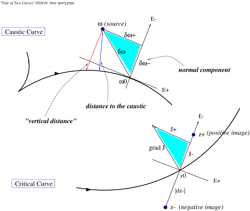
Figure 1: Quadratic behavior of the lens equation near a critical point $z_{\circ}$ where $J_{-}(z_{\circ})\not\approx 0$:  The criticality defines the image line  $dz\parallel\pm E_{-}(z_{\circ})$ and the source line  $\delta\omega\parallel\bar{\partial}J(z_{\circ})$, and the lens equation becomes a real symmetric quadratic equation from the image line to the source line:  $\delta\omega={1\over 2}\bar{\partial}J~{}dz_{-}^{2}$. There are two images when $\delta\omega/\bar{\partial}J>0$, and no images when $\delta\omega/\bar{\partial}J<0$. Here  $\delta\omega\parallel\bar{\partial}J$, and $\omega$ generates two images $z_{\pm}$ near the critical point $z_{0}$. The positive image at $z_{+}$ is in the direction of $\nabla J$, and the negative image at $z_{-}$ is in the opposite direction. The amplification of the images is $\sqrt{(4\delta\omega_{-}J_{-})^{-1}}$, and both the shortest distance and the “vertical distance” differ from the “truely relevant distance” $|\delta\omega_{-}(\omega_{\circ})|$.

Gaudi & Petters (2001) warns the readers, “there are not many people who know that the distance is not the shortest distance but the vertical distance.” The distance $\delta$ is neither the shortest distance nor a vertical distance as is described in the abstract and illustrated in Fig. 1. When $\delta$ can be approximated by the shortest distance, the “vertical distance” converges to $\delta$ as well.

Regurgitation of RB99:

In the case of the binary lens in rb99.Fig.1 where the two masses are comparable and their separation is $\sim{\cal O}(1)$ (where $1$ refers to the Einstein ring radius of the total mass), the gradient of the Jacobian determinant $|\nabla J|\sim{\cal O}(1)$. Equation rb99.13 reads as follows when $dz_{+}$ is reinstated.

$$\delta\omega_{-}=\delta\omega_{2-}={1\over 4}\left(J_{-}(dz_{-}^{2}-dz_{+}^{2})+2J_{+}dz_{+}dz_{-}\right)$$ (2)

If we assume the linear approximation for $dz_{+}$ as in rb99, the quadratic equation in $dz_{-}$ can be solved in terms of $dz_{+}$ and $\delta\omega_{-}$.

$$dz_{-}=-{J_{+}\over J_{-}}dz_{+}\pm\sqrt{{|\nabla J|^{2}dz_{+}^{2}\over J_{-}^{2}}+{4\delta\omega_{2-}\over J_{-}}}$$ (3)

Since $dz_{-}$ is real, as we have emphasized that $E_{\pm}$ decomposition components are real variables above and in equation (51), $dz_{-}$ has solutions when the inside of the square root is non-negative (rb99.14).

$$\delta\omega_{-}\partial_{-}J+|\partial J|^{2}dz_{+}^{2}\geq 0$$ (4)

The degenerate solution for which the equality of equation (4) holds amounts to a shift along the critical curve.

$$dz_{-}=-{J_{+}\over J_{-}}dz_{+}\quad\Rightarrow\qquad J_{+}dz_{+}+J_{-}dz_{-}=0$$ (5)

If $z_{\circ}$ is a critical point, then $z_{\circ}^{\prime}\equiv z_{\circ}+dz_{+}(E_{+}-J_{+}E_{-}/J_{-})$ is also a critical point.

We rewrite $z_{\circ}+dz$ as a vector deviated from $z_{\circ}^{\prime}$ such that $z_{\circ}+dz=z_{\circ}^{\prime}+dz^{\prime}$. Then, $dz^{\prime}$ is a vector in the direction of $\pm E_{-}(z_{\circ})$.

$$dz^{\prime}(z_{\circ}^{\prime})=\pm E_{-}(z_{\circ})~{}\sqrt{{|\nabla J|^{2}dz_{+}^{2}\over J_{-}^{2}}+{4\delta\omega_{2-}\over J_{-}}}$$ (6)

If $\omega_{\circ}=\omega(z_{\circ})$ is the caustic point corresponding to the “old” critical point $z_{\circ}$, then $\omega_{\circ}^{\prime}\equiv\omega_{\circ}+2dz_{+}E_{+}(z_{\circ})$ is a new caustic point because $E_{+}(z_{\circ})$ is tangent to the caustic curve. We can easily calculate the new caustic point $\omega_{\circ}^{\prime}$ up to the second order. Let’s start for clarity with the general second order expansion in $d\bar{z}$ in equation (48).

$$\delta\omega_{2}\equiv{1\over 2}\bar{\partial}\bar{\kappa}d\bar{z}^{2}={1\over 2}(-\bar{\partial}J)(dz_{+}-idz_{-})^{2}\$$ (7)

The second equality is obtained by using $\bar{\partial}J=-\kappa\bar{\partial}\bar{\kappa}$, $E_{\pm}$-decomposition $dz=dz_{+}E_{+}+dz_{-}E_{-}$, and miscellaneous relations such as $E_{-}=iE_{+}$ that can be found in rb99 and section 2. In order to get the expression for the caustic point, we apply the condition $0=J_{+}dz_{+}+J_{-}dz_{-}$ and get $\delta\omega$ parameterized by $dz_{+}$.

$$\delta\omega=\delta\omega_{+}E_{+}+\delta\omega_{-}E_{-}=\left(2dz_{+}+{1\over 4}{|\nabla J|^{2}\over J_{-}^{2}}J_{+}dz_{+}^{2}\right)E_{+}-{1\over 4}{|\nabla J|^{2}\over J_{-}^{2}}J_{-}dz_{+}^{2}~{}E_{-}$$ (8)

We rewrite the equations for $\delta\omega_{+}$ and $\delta\omega_{-}$ as follows for later use.

$$0 = (\delta\omega_{+}-2dz_{+})J_{-}+J_{+}\delta\omega_{-}$$ (9)

$$\delta\omega_{-} = -{1\over 4}{|\nabla J|^{2}\over J_{-}}dz_{+}^{2}$$ (10)

It should be clear that the role of $dz_{+}$ is mainly to cause a migration of the cautic point and critical point from $\omega_{\circ}$ and $z_{\circ}$ to new ones $\omega_{\circ}^{\prime}$ and $z_{\circ}^{\prime}$ respectively. In order to see the uncluttered picture of the local behavior of the lens equation near a critical point, we set $dz_{+}=0$.

-1.   In Details We Trust: Brutally Honest Interpretations

If $dz_{+}=0$, $dz=dz_{-}E_{-}$, and from equation (61),

$$\delta\omega_{1\pm}=0\ ; \delta\omega_{2\pm}={1\over 4}dz_{-}^{2}J_{\pm}\$$

$$\Longleftrightarrow\qquad\delta\omega = \delta\omega_{2+}E_{+}+\delta\omega_{2-}E_{-}={1\over 2}\bar{\partial}J~{}dz_{-}^{2}\ .$$

This is the quadratic behavior of the lens equation near a critical point. The role of the critical direction is clear. If $z_{\circ}$ is a critical point, two images separated along the critical direction at $z=z_{\circ}\pm|dz_{-}|E_{-}$ are from a same source. If $\omega_{\circ}$ is the caustic point corresponding to $z_{\circ}$ under the lens equation, then the position of the source, $\omega=\omega_{\circ}+\delta\omega$, that produces the two images is such that the shift $\delta\omega$ is in the same direction as the gradient of the Jacobian determinant $\nabla J=(J_{+},J_{-})$ at $z_{\circ}$. See Fig. 1. We refer to this caustic point $\omega_{\circ}$ as the preferred caustic point for $\omega$.

Question :   Suppose $\omega$ is an arbitrary source position near the caustic curve. Then, it is conceptually straightforward how to find the images of $\omega$ near the critical curve.

Solution :   We find a caustic point $\omega_{\circ}$ such that $\delta\omega=\omega-\omega_{\circ}$ is parallel to $\bar{\partial}J$ (or $\nabla J$) at $z_{\circ}$ where $z_{\circ}$ is the critical point that corresponds to $\omega_{\circ}$.

Then, two images of $\omega$ can be found in the critical direction from the critical point $z_{\circ}$:  $z=z_{\circ}\pm|dz_{-}|E_{-}$ where

$$|dz_{-}|=\sqrt{4\delta\omega_{2+}\over J_{+}}=\sqrt{4\delta\omega_{2-}\over J_{-}}=\sqrt{2\delta\omega\over\bar{\partial}J}\ .$$ (11)

The two images have opposite parities and same magnification as reflected in the signs and absolute value of the Jacobian determinant at the image positions (rb99.11).

$$J(z_{\circ}+dz)=dJ=dz_{-}J_{-}=\pm|dz_{-}||J_{-}|=\pm\sqrt{4\delta\omega_{2-}J_{-}}$$ (12)

If $\delta\omega$ is antiparallel to $\bar{\partial}J$, the inside of the square roots in equation (11) is negative, and $\omega$ generates no images near the critical curve.

1. Once the directionalities of the image line ($\pm E_{-}$) and source line ($\bar{\partial}J$) are determined, the lens equation becomes a real symmetric quadratic equation from the image line to the source line. The lens equation from the image line to the source line has two solutions for  $\delta\omega\partial J>0$ (real and positive), no solutions for  $\delta\omega\partial J<0$ (real and negative), and degenerate at the critical point where  $\delta\omega\partial J=0$. It is exactly like the simple real quadratic equation $y=ax^{2}$: $y=ax^{2}$ has two solutioins for  $ay>0$, and no solutions for  $ay<0$. At the critical point $x=0$ where $dy/dx=0$, the solutions are degenerate.

   It should be worth emphasizing that the image line ($\pm E_{-}$) and source line ($\bar{\partial}J$) are not orthogonal to each other even though it may be tempting to imagine so because of our perception from the graph $y=ax^{2}$ which we are accustomed to draw in orthogonal grids.

2. In fact, the second order approximation fails where the image line and the source line are orthogonal ($J_{-}=0$). Since equation (3) fails where $J_{-}=0$, we need to consider the third order terms. The underlying reason can be seen in that the second order terms accomodate only a migration along the critical curve as is clear from equation (12).

3. Fig. 1 clearly shows that the larger the angle between $\nabla J$ and $E_{-}$, the more tangentially the images $z_{\pm}$ are shifted from $z_{\circ}$, and the smaller the normal distance of the images from the critical curve which determines the $J$-value ($dJ$). If we consider a small stellar disk near the caustic curve, the images will be extensively elongated along the critical curve where $J_{+}>J_{-}$.

4. Geometrically, $J_{-}=0$ means that the critical direction is tangent to the critical curve. Let’s consider the lens equation as a mapping restricted to the critical curve. Then, the restricted mapping is stationary or critical where $J_{-}=0$. In other words, the caustic curve as an integral curve of the tangent develops a point (cusp) where $J_{-}=0$ because the “speed” vanishes as in the trajectory of a pendulum at the maximum gravitational potential.

   $$\int d\omega=\int d\omega_{+}E_{+}+d\omega_{-}E_{-}=\int_{critical\ curve}2dz_{+}E_{+}$$ (13)

   $$0=dJ=dz_{+}J_{+}+dz_{-}J_{-}=dz_{+}J_{+}\quad\Rightarrow\quad\delta\omega_{+}=2dz_{+}=0$$ (14)

   The cusps are the only singularities on the caustic curve. That is because the lens equation is smooth on the critical curve, and the critical curve is smooth. (A critical curve can have bifurcation points that are four-prong vertices, and the caustic curve develops cusps; see RBCPLX). Thus, the caustic curve is smooth except at the critical points where the restricted mapping is stationary.

5. If $J_{+}=0$, the two normals to the critical curve and the caustic curve coincide. $|J_{-}|=|\nabla J|$ and $|\delta\omega_{2-}|=|\delta\omega|$. The image line (the line connecting the two images) is perpendicular to the critical curve, and $|\delta\omega|$ is the (shortest) distance from $\omega$ to the caustic point onto which the critical point that disects the image line is mapped under the lens equation. There is no need to be an alarmist for that the second term in equation (11) is not well defined where $J_{+}=0$. Both $\delta\omega_{2+}$ and $J_{+}$ vanish, and the second term is not sufficient to offer a finite number when $J_{+}=0$, but there is no conceptual outrage. The last two expressions are equivalent and offer the value of $|dz_{-}|$.

What is $\delta$ in $J^{-1}\propto\sqrt{\delta^{-1}}$?

In this second order approximation, $J(\omega)$ is derived from two relations.

$$J=J_{-}~{}dz_{-}\ ;\qquad dz_{-}=\pm\sqrt{2\delta\omega\over\bar{\partial}J}$$ (15)

The first equation holds since we chose the critical point $z_{\circ}$ such that $z_{\circ}$ intersects the image line (along the critical direction). In fact, $z_{\circ}$ bisects the image line. The second equation depends on (the square root of) the ratio of $\delta\omega$ to $\bar{\partial}J$, and the ratio can be expressed variously as shown in equation (11). Thus, the title question “What is $\delta$ in $J^{-1}\propto\sqrt{\delta^{-1}}$?” is not a question well posed because the answer depends on the choice of the multiplication function. However, given the preferential appearance of $J_{-}$ in $J=dJ=J_{-}~{}dz_{-}$ (since $dz_{+}=0$ here), we can agree to implicitly refer to $4J_{-}$ as the multiplication function. Then, the “truly relevant distance” is $\delta=|\delta\omega_{-}(\omega_{\circ})|$ and is shown in Fig. 1 in comparison to the (shortest) distance to the caustic and “vertical distance” (to the cautic curve).

Answer:   If we choose $4J_{-}$ as the multiplification factor, the distance $\delta$ is given by $|\delta\omega_{2-}|$ where $\delta\omega_{2-}$ is the normal component of $\delta\omega=\omega-\omega_{\circ}$ and the caustic point $\omega_{\circ}$ is chosen such that $\delta\omega\parallel\bar{\partial}J$.

-1.1   Non-preferred Caustic Point as the Origin: $\omega_{c}\not=\omega_{\circ}$

If we choose an arbitrary caustic point $\omega_{c}$ in the caustic region of interest as the origin of a power expansion, then $\delta\omega=\omega-\omega_{c}$ where $\omega$ is a source position in the caustic region. If we let $x\equiv\delta\omega_{+}$ and  $y\equiv\delta\omega_{-}$;  $u\equiv\delta z_{+}$ and  $v\equiv\delta z_{-}$;  $a\equiv J_{+}$ and  $b\equiv J_{-}$ for visual simplicity, then, the second order lens equations (61) in the neighborhood of $\omega_{c}$ are rewritten as follows.

$$x-2u = -{1\over 4}\left(a(u^{2}-v^{2})+b~{}2uv\right)$$ (16)

$$y = -{1\over 4}\left(b(u^{2}-v^{2})-a~{}2uv\right)$$ (17)

One combination of the two equations reads as follows.

$$(bx-ay-2bu)=-{1\over 4}(a^{2}+b^{2})~{}2uv$$ (18)

Since we have chosen a non-preferred caustic point, the image position solutions will include shifts along the critical curve from the origin $z_{c}$ where $\bar{\partial}J$ is calculated. In this second order approximation, the change of $J_{\pm}$ along the critical curve can not be incorporated because higher order derivatives of the Jacobian determinants become involved in the third order terms and higher. Thus, $\nabla J$ is implicitly considered constant in the neighborhood of $z_{c}$.

Linear Approximation for $dz_{+}$:

We take the linear approximation as in rb99.12 (but correctly) by ignoring the RHS.

$$(bx-ay)=2bu$$ (19)

In rb99.12, the second term $(-ay)$ in equation (19) is missing. This missing term causes what amounts to an intrinsic violation of the second order nature of the equations or of the proper handling of a triangular matrix. Since the linear contribution for $y$ vanishes, the second order contribution to $y$ feeds back to $x$ through the second order contributions. In order to cut at the linear order of $\delta\omega_{\pm}$, we need to fully incorporate these contributions in the second order in $dz_{\pm}$. For example, if $x$, $y$, and $u$ are an order of $10^{-3}$ as in a typical case of a main sequence source star in the Galactic bulge lensing, then $v$ is an order of $\sqrt{10^{-3}}$ and $\delta\omega_{2+}$ is of the same order as $\delta\omega_{1+}$. In fact, we know that we can choose $\omega_{\circ}$ for the caustic point such that $\delta\omega_{1+}$ vanishes while $\delta\omega_{2+}$ doesn’t. Once $u$ is determined by the linear equation in (19), we can find $v$ in terms of $u$ and $y$ from equation (19), which is the same as rb99.13 with $dz_{+}$ reinstated.

$$v=-{a\over b}u\pm\sqrt{{a^{2}+b^{2}\over b^{2}}u^{2}+{4y\over b}}$$ (20)

The first term in the RHS describes a shift along the critical curve, and so the non-vanishing contribution to $J=dJ=au+bv$ comes from the second term in the RHS.

$$J=\pm b\sqrt{{a^{2}+b^{2}\over b^{2}}u^{2}+{4y\over b}}$$ (21)

We can rewrite it in terms of the original notations.

$$J(\omega) = \pm\sqrt{4J_{-}\Delta\omega_{-}}$$ (22)

$$\Delta\omega_{-} \equiv \delta\omega_{-}+{(\nabla J)^{2}\over 16J_{-}}\left(\delta\omega_{+}-{J_{+}\over J_{-}}\delta\omega_{-}\right)^{2}$$ (23)

If we stare at the solutions in (19) through (23) for a moment, a few things are clear.

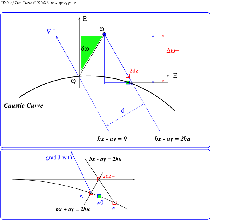
Figure 3: Non-preferred caustic point $\omega_{c}$ as the origin. The value of multiplication function $J_{-}$ is calculated at the origin, and $\Delta\omega_{-}$ is the normal component of $\delta\omega-\delta\omega(J=0)$. The bottom panel compares the caustic points: $w+$ is the correct caustic point for given $2dz_{+}$; $w-$ is the caustic point defined by the line $bx-ay=2bu$ and was referred to as the approximate preferred caustic point for $\omega$; $w0$ is the derived preferred caustic point for $\omega$ in the linear approximation of $dz_{+}$.

1. The line (or graph) defined by $(bx-ay)=2bu$ in equation (19) is parallel to $\nabla J$. Thus, the linear approximation for $dz_{+}$ in equation (19) implies that the line $(bx-ay)=2bu$ should connect the source position $\omega$ and the approximate preferred caustic point. The approximate preferred caustic point is marked as $w-$ in Fig. 3. The line $(bx-ay)=2bu$ intersects the $x$-axis at $x=2u$ and is at a distance $d$ from the line defined by $(bx-ay)=0$ as shown in the same figure.

   $$d={2u\over\sqrt{a^{2}+b^{2}}}={|2dz_{+}|\over|\nabla J|}={1\over|\nabla J|}\left|\delta\omega_{+}-{J_{+}\over J_{-}}\delta\omega_{-}\right|$$ (24)

2. The approximate preferred caustic point determined by the line $(bx-ay)=2bu$ can be found by solving equations (20) and (30) simultaneously.

   $$x \approx 2u-{a(a^{2}+b^{2})\over 16b^{2}}~{}(2u)^{2}~{}\approx~{}2u$$

   $$y=-{a^{2}+b^{2}\over-16b}x^{2} \approx {a^{2}+b^{2}\over 4b}u^{2}\approx{a^{2}+b^{2}\over 16b}\left(\delta\omega_{-}-{J_{+}\over J_{-}}\delta\omega_{+}^{2}\right)^{2}$$

   The approximations for $x$ and accordingly for $y$ have been made based on the validity condition for $x$ in equation (29). The caustic point is marked by $w0$ in Fig. (3) and will be referred to as $\omega_{c_{0}}$ in this text.
   

   What is $\Delta\omega_{-}$?

   If we consider $\delta\omega(\omega_{c_{0}})\equiv\omega-\omega_{c_{0}}$, then $\Delta\omega_{-}$ in equation (23) is nothing but the normal component of $\delta\omega(\omega_{c_{0}})$.

   $$(\omega-\omega_{c_{0}})\cdot E_{-}=(\delta\omega_{-}-y)~{}\approx~{}\delta\omega_{-}+{a^{2}+b^{2}\over 16b}\left(\delta\omega_{-}-{J_{+}\over J_{-}}\delta\omega_{+}^{2}\right)^{2}$$ (25)

   We impose an implicit understanding that the caustic point $\omega_{c_{0}}=\omega(J=0)$ is to be found in the direction of the normal $\bar{\partial}J$ calculated at $z_{c}$ where the power series expansion of the lens equation is made.

   $$\Delta\omega_{-}=(\omega-\omega(J=0))\cdot E_{-}=\delta\omega_{-}-\delta\omega_{-}(J=0)$$ (26)

   If $\omega_{c}$ coincides with $\omega_{c_{0}}$, then $\omega_{c}=\omega_{c_{0}}=\omega_{\circ}$, and $\Delta\omega_{-}=\delta\omega_{-}$.

3. The causic curve in the second order approximation satisfies equations in (10), and the resulting quadratic equation for the caustic curve is written in equation (27). If $(x,y)$ is a caustic point, then $x$ and $y$ lie on the line defined by the first equation in (10), and the line intersects the $x$-axis at $x=2u$ as shown in Fig. 3. The caustic point for the given value of $u$ differs from the caustic point determined by the line $(bx-ay)=2bu$, and the former is marked as $w+$ in Fig. 3. It should be clear that $w0$ is always located between $w+$ and $w-$. The linear approximation for $dz_{+}$ in equation (19) is valid when $w+\approx w0\approx w-$ with the second order approximation.

4. Error from Nonlinear Correction for $dz_{+}$:

   In order to test the goodness of the linear approximation for $dz_{+}$, let’s examine the intersection point of the second order equation (17) with the $x$-axis. If we set $y=0$, equations of (17) leads to the following.

   $$v = {1\over b}(-a\pm\nabla J)u\ ;$$

   $$x = 2u+{a^{2}+b^{2}\over 8b^{2}}(a\pm|\nabla J|)~{}(2u)^{2}$$

   As we mentioned before, $u$ is sufficiently smaller than 1 (Einstein ring radius), and the second term can be ignored unless it is near a cusp where $b=J_{-}\approx 0$ or $|\nabla J|$ is large as in the case of small caustics such as planetary caustics we will briefly discuss below.

Quadratic Caustic Equation:

Now, we write out the quadratic caustic equation and its validity used in the previsous section. The equation for the caustic curve can be obtained from equation (17) and the condition $0=dJ=J_{+}dz_{+}+J_{-}dz_{-}=au+bv$.

$$-16by={a^{2}+b^{2}\over b^{2}}(bx+ay)^{2}\quad\Rightarrow\quad bx=-ay\pm\sqrt{-16b^{3}y\over a^{2}+b^{2}}$$ (27)

1. The equation is non-linear in $y$, but we can confirm that the origin ($x=y=0$) is indeed a critical point ($dy/dx=0$).

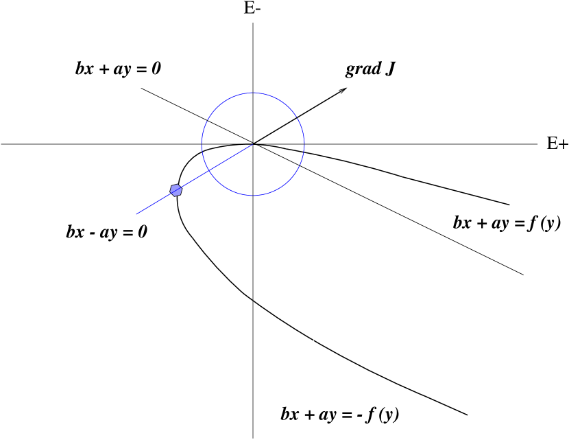
Figure 4: The caustic curve in the second order approximation satisfies a quadratic equation between $y$ and $bx+ay$. Here $f(y)=\sqrt{-16yb^{3}/(\nabla J)^{2}}$. The equation is a valid description of the original caustic curve in the neighborhood (here circled for illustration) where $|ay|$ is negligible in comparison to the other two terms $bx$ and $f(y)$ and becomes a quadratic function between $y$ and $x$.

2. Where $by<0$, every $y$ has two solutions. See Fig. 4.

3. The slope $dy/dx$ diverges where the “source line” (parallel to $\nabla J$) intersects with the caustic curve given by equation (17).

   $$y_{\infty}=-{4b^{3}\over a^{2}(a^{2}+b^{2})}\quad\Rightarrow\qquad bx_{\infty}-ay_{\infty}=0\ .$$ (28)

   This indicates where equation (17) fails to describe the original caustic curve. We can say that the quadratic equation (17) (not necessarily quadratic in the orthogonal coordinate variables $x$ and $y$) is valid where $|y|<<|y_{\infty}|$, or equivalently where $(bx)$ dominates over $(-ay)$. From this condition, we get a criteria for $|x|$.

   $$|x|<<{4\over|J_{+}|}\left(J_{-}\over\nabla J\right)^{2}$$ (29)

   For small $x$ where $|ay|<<|bx|$, equation (17) becomes a simple quadratic equation.

   $$-16by=(a^{2}+b^{2})x^{2}\quad\Leftrightarrow\quad-16J_{-}\delta\omega_{-}=|\nabla J|^{2}\delta\omega_{+}^{2}$$ (30)

4. If $J_{-}=0$, the range $|x|<<0$. In other words, the quadratic equation for the caustic curve is completely invalid at the cusp. It is consistent with that the second order approximation of the lens equation fails where $J_{-}\approx 0$.

   If $J_{-}=0$, the source line $bx-ay=0$ becomes $y=0$, and so $dx/dy=0$ at $y=0$. This is another way to look at the failure of the quadratic equation near a cusp.

5. If $J_{+}=0$, the range of $|x|$ in equation (29) is unlimited. That is directly because $(-ay)$ term vanishes and so $bx$ term dominates. If we look at Fig. 4, $bx+ay=0$ and $bx-ay=0$ become degenerate, and the quadratic caustic curve in Fig. 4 becomes symmetric: $bx=\pm f(y)$, or $-16by=(\nabla J)^{2}x^{2}$.

1 A Single Lens with Constant Shear

In 1979, the first double quasar Q0957+561A,B (Walsh, Carswell, and Weymann 1979) was discovered and interpreted as two images of one quasar gravitationally lensed by a galaxy (or a group of galaxies) as a continuum distribution of mass. Chang and Refsdal (1979) considered the effect of “image splitting” of an image due to the granularity of a single star which happens to be near the astrometric (or transverse) position of the image. The angular scale of the “image splitting” of an image of a quasar (at a cosomological distance) by a stellar mass object is an order of microarcsecond while the two images Q0957+561A,B are separated by $\sim 6$ arcseconds. Thus, the nearity of the would-be image lensed by the galaxy to the (microarcsecond) lensing star amounts to the precision level of $\sim 10^{-6}$, and the gravitational influence of the lensing galaxy in the small area defined by the microarcsecond lensing radius of the star can be considered constant.

The equation for a single point lens with constant shear entails a preferred direction and that is the direction of the (effective) mass which generates the constant shear in the small area of interest around the single point mass. In other words, constant shear is intrinsically an approximation and can be obtained by taking large mass and large distance limits of more physically well-defined mass distributions.

As a concrete example, let’s take a large mass parity limit of the binary lens in Eq. (43). The lens equation has been normalized by $R_{E}$ the Einstein ring radius of the total mass, and we can suppose that $\epsilon_{1}<<\epsilon_{2}$ such that $\epsilon_{1}$ is the mass fraction of the (microarcsecond) lensing star. If we rescale the lens equation by the Einstein ring radius of the stellar mass $\epsilon_{1}$, then $\epsilon_{1}=1$, and $\epsilon_{2}>>1$. We can set $x_{1}=0$ (choice of the coordinate origin), and then the microarcsecond lensed images will be around $|z|\sim 1$. In order for the lensing by the larger mass not to dominate the lensing behavior of the images around $|z|\sim 1$, the bending angle by the larger mass must be the order of the bending by the stellar mass $\epsilon_{1}$ or smaller. For images around $|z|\sim 1$, $|x_{2}|>>|z|$, and the lens equation can be rewritten as follows.

$$\omega-{\epsilon_{2}\over x_{2}}=z-{\epsilon_{1}\over\bar{z}-x_{1}}+{\epsilon_{2}\bar{z}\over x_{2}^{2}}+{\cal O}(x_{2}^{-3})\ .$$ (31)

We note that $\sqrt{\epsilon_{2}}\sim R_{E}$ is the Einstein ring radius of the mass $\epsilon_{2}$ as a single lens. If $\epsilon_{1}$ is at a distance of $\sim R_{E}\approx\sqrt{\epsilon_{2}}$ from $\epsilon_{2}$, then the source at $\omega\approx\epsilon_{2}/x_{2}$ produces images at whose positions the influence of the large mass $\epsilon_{2}$ can be considered a constant shear of order 1:  $\gamma\equiv\epsilon_{2}/x_{2}^{2}\sim{\cal O}(1)$.

The constant shift $\epsilon_{2}/x_{2}$ indicates that the emission source is near the position of the large mass $x_{2}>>1$ for the images around with $|z|\sim{\cal O}(1)$, and the effect of the single point mass is to “split” the would-be image around the Einstein ring of the large mass. The outer image is splitted by a quadroid and the inner image is splitted by two trioids. These behavior can be very easily understood from the binary lens equation which is a physically well-defined closed system.

It is customary to ignore the constant shift $\epsilon_{2}/x_{2}$ in a lens equation with a constant shear.

$$\omega=z-{1\over\bar{z}}+\gamma\bar{z}$$ (32)

This equation is often referred to as Chang-Refsdal equation (e.g., SEF) and the constant shear term points to the positive direction of the $x$-axis. This particular directionality has been inherited from 1) the binary equation (43) where the lens axis is along the real axis and 2) the implicit assumption in the derviation of equation (31) that the larger mass was in the positive direction. In general, the constant shear coefficient $\gamma$ would be a complex number $\gamma\equiv\epsilon_{2}/\bar{x}_{2}^{2}$ half whose phase angle points to the effective direction of the larger mass that generates the constant shear.

It is noteworthy that the second term in equation (32) due to the (microarcsecond) lensing star is also a shear term, and this shear term vanishes at $\infty$ – far away from the mass that generates the shear. However, the constant shear does not vanish at $\infty$. It is in a sense a reminder that constant shear is inherently an expression of approximation, and the lens equation with a constant shear should be treated as an incomplete equation which requires auxiliary assumptions or interpretations to be a physically viable model for a lensing system. For example, the “source position” in equation (32) can not be the position of the source because the “source position” is in practice the position of the would-be image generated by the larger mass that effects the constant shear around the (microarcsecond) lensing star.

In order to see the effect of the constant shear, let’s remove the point mass of the star from equation (32).

$$\omega=z+\gamma\bar{z}\ ;\qquad J=1-|\gamma|^{2}$$ (33)

The equation is linear, and the constant shear generates only one image. The magnification ($|J|^{-1}$) and parity (sign of $J$) of the image is the same everywhere irrelevantly of the position of the “source”, which is arguably the essence of a constant shear.

$$z={\omega-\gamma\bar{\omega}\over 1-\gamma^{2}}$$ (34)

The image is contracted in the direction of the shear $\gamma$ by a factor $(1+\gamma)^{-1}$ and elongated in the orthogonal direction by a factor $(1-\gamma)^{-1}$. The distortion is universal where the constant shear approximation applies. In weak lensing where the shape of the objects is one of the measurable and interpretable quantities, such systematic distortions due to lensing can be detected and are being pursued to study large scale structures that may shed light on the history and make-up of the universe including dark stuff (matter, energy, essence, extra dimensions, topological defects, … , even though it is unclear whether the essence is essential, extra dimensions are most likely a fundamental ingredient but for the time being a tantalizing yet unproven conjecture, and the exact nature of the topological defects or objects may turn out to be as fascinating as the existential properties of the space or the baryon number and remain illusive for a long time to come). How well one can determine the shear distribution crucially depends on the shape resolution and statistics of the shape objects. A degree scale large format space imager Galactic Exoplanet Survey Telescope will be a fitting explorer even though the wings have been clipped again.

1.1 The $\kappa$ Field of the Single Lens with Constant Shear

The linear differential behavior is insensitive to the constant shift of the source position and can be discussed routinely as usual. As in the case of $n$-point lenses (Rhie, 1997; Rhie & Bennett, 1999; Rhie, 2001), the linear differential behavior of the lens equation (31) is completely determined by one analytic function $\kappa$, and so we use and follow the facts, conventions, and analysis patterns in the references (RBCPLX from here on). The Jacobian of the lens equation can be written as follows where the $2\times 2$ matrix indicates that the underlying space of the complex plane is a 2-d linear space.

$${\cal J}=\pmatrix{1\ \bar{\kappa}\cr\kappa\ 1}\ ;\qquad\kappa\equiv{\partial\bar{\omega}}\equiv{\partial\bar{\omega}\over\partial z}={1\over z^{2}}+\gamma$$ (35)

The condition for criticality, $|\kappa|=1$, is a second order analytic polynomial equation, and so the phase angle of $\kappa$ changes by $2\pi$ along the critical curve.

$$\kappa=e^{i2\varphi}\ ;\qquad\Delta\varphi=2\pi$$ (36)

Thus, the total topological charge of the critical loops or caustic loops is $\sum|e|=1$, and the caustic is made of one 4-cusped quadroid or two 3-cusped trioids. The depiction can be found in Chang (1984) and also in SEF.Fig.8.8. There are two limit points (where $\kappa=0$) on the imaginary axis (orthogonal to the direction of the constant shear) at $z=\pm i/\sqrt{\gamma}$, and the trioids enclose the limit points.

$$J(z)=1-|\kappa(z)|^{2}\leq 1\ ;\qquad J(\infty)=1-\gamma^{2}$$ (37)

The Jacobian determinant $J(z)$ of this lens equation with a constant shear is bounded by $J(z)\leq 1$. The maximum holds at the finite limit points $z=\pm i/\sqrt{\gamma}$ but not at infinity. In fact, the critical curve can pass through the infinity and the image at infinity can be infinitely bright. This unphysical behavior derives from that the lens equation with a constant shear is accommodated by an infinitely large mass at infinity when the lens equation is extended to the whole lens plane. This behavior is easy to understand when seen as an approximation of the binary lens. The critical points at infinity correspond to the bifurcation points where the topology of the critical curve changes from one loop to two loops. At the same time, the topology of the caustic curve changes from one quadroid to two trioids.

1.2 Images

We have derived the lens equation (32) of a single lens with a constant shear from the binary lens equation and can read off some of the basic properties of the equation following the recipes developed for binary (or $n$-point) lenses briefly reviewed in the following section.

1. The caustic loops are simple loops. In other words, they neither self-intersect nor nest. Thus, the source plane accomodates only two domains: ${\cal D}^{\circ}$ (outside) and ${\cal D}^{1}$ (inside).

2. There are two images outside the caustic loop(s). One only needs to examine the number of images of $\omega=\infty$ because the outside domain ${\cal D}^{\circ}$ includes $\infty$.

3. A source inside a caustic loop (${\cal D}^{1}$) produces four images, and the caustic loop itself produces three image loops one of whose is the critical curve. The caustic curves have cusps, and so the two “non-critical curves” have kinks at the corresponding points unless they are precusps. However, the critical curve is smooth because the inverse mapping of the lens equation from the caustic curve to the critical curve is singular at the cusps the singular points. Precusps are bifurcation points of the critical curve and “non-critical curves” (see Fig.10 in Rhie (2001)).

The constant shear breaks the axial symmetry of the single lens but leaves a residual reflection symmetry as is familiar from binary lenses (Rhie & Bennett, 2001). If the source is on the lens axis, $\omega=\bar{\omega}$, there are two images on the the lens axis, $z=\bar{z}$, and two extra images on a circle $|z|^{-1}=\sqrt{1-\gamma}:\gamma>1$. The lens equation subject to $\omega=\bar{\omega}$ leads to the following equation.

$$0=(z-\bar{z})\left(1-{1\over|z|^{2}}-\gamma\right)$$ (38)

1. $z=\bar{z}$:   The two images on the lens axis are very much like the two images of a single lens that form on the line defined by the positions of the lens and source.

   $$\omega=z(1+\gamma)-{1\over z}\quad\Longrightarrow\quad\left[{\omega\over\sqrt{1+\gamma}}\right]=\left[\sqrt{1+\gamma}~{}z\right]-{1\over\left[\sqrt{1+\gamma}~{}z\right]}$$ (39)

   The second equation shows the correspondence with the equation of a single lens.

2. $|z|^{-2}=1-\gamma\ (>0)$:   The two images are on the circle of radius $|z|=1/\sqrt{1-\gamma}$ centered at the lens position (here the origin) where the real component of the image positions is given by a simple linear scaling of the source position from the lens.

   $$\omega=2\gamma~{}Re(z)\ :\qquad\gamma>1\ \ {\rm and}\ \ |Re(z)|\leq{1\over\sqrt{1-\gamma}}$$ (40)

   When $\gamma<1$, the caustic curve is a quadroid intersecting the lens axis. The cusps of the quadroid are easily calculated:  two are on the real axis (the lens axis) and has $\kappa=1$, and the other two are on the imaginary axis and has $\kappa=-1$.

   $$\omega_{cusp}={\pm 2\gamma\over\sqrt{1-\gamma}}\ ,\qquad{\pm i~{}2\gamma\over\sqrt{1+\gamma}}$$ (41)

   The two images on the circle exist when $\omega$ is inside the quadroid, which can be easily read off from equations (40) and (41). The Jacobian determinant of the images on the circle is given as follows.

   $$J=4\gamma(1-\gamma)\sin^{2}\theta\ \geq 0\ :\qquad z={e^{i\theta}\over\sqrt{1-\gamma}}$$ (42)

   The images on the circle are positive images except at the cusps. At the cusps on the real axis given in equation (41), $J=0$, and the circle is tangent to the critical curve. We can easily check that the images on the real axis are inside the critical curve and so are negative images. The total parity of the images of a single lens with a constant shear is zero.

   When $\gamma>1$, the caustic curve is made of two triods enclosing the two limit points, and the two caustic loops are off the lens axis. Thus, $\omega=\bar{\omega}$ has only two images and they have opposite parities exactly as in the case of a single lens.

The fact that the two extra images are on a circle deserves a modest attention. If we decrease the effect of the constant shear, $\gamma\rightarrow 0$, the circle approaches the critical curve of the single lens of radius 1, namely the Einstein ring radius:  $J\rightarrow 0$ and $|z|\rightarrow 1$. In general, Einstein ring, critical curve, and image ring are all distinct. Einstein ring determines the (transverse) distance scale of lensing. Critical curve is where the Jacobian determinant of the lens equation vanishes, images are degenerate, and the magnitude of the images diverge. Image ring is a proxy ring which a finite size source fallen inside a caustic loop produces, and its shape and intensity depends on the caustic structure and the relative position of the source. In the case of a single lens, they all converge to one ring. In the case of the single lens with a constant shear, its proximity to a single lens makes the image ring quite circular. In fact, the same line of thought offers a valid intuition for caustics of higher multiple lenses when the effect of the lens elements but one can be considered a long distance effect.

2 Binary Equation, Quasi-Analytic Equations

The binary lens equation is written as follows (see RBCPLX, references therein, or others).

$$\omega=z-{\epsilon_{1}\over\bar{z}-x_{1}}-{\epsilon_{2}\over\bar{z}-x_{2}}\ ,$$ (43)

where $\omega$, $z$, and $x_{j}:j=1,2$ are the positions of a source, an image, and the lens elements of fractional masses $\epsilon_{j}:j=1,2$ in the two dimensional sky as a complex plane. We have chosen the lens axis to be along the real axis so that $x_{1}$ and $x_{2}$ are real, and the unit distance scale is given by the Einstein ring radius $R_{E}$.

$$1=R_{E}=\sqrt{4GMD}\ ;\qquad{1\over D}={1\over D_{1}}+{1\over D_{2}}$$ (44)

where $D$ is the reduced distance.

When there are $n$ point lens elements where $n>2$, we only need to extend the range of the index to $j=1,2,...,n$ and replace the lens position vectors to $\bar{x}_{j}$ because we can not line them up all on the real axis. The form of the Jacobian matrix in equation (35) applies to any quasi-analytic lens equation, and $\kappa\equiv\partial\bar{\omega}$ is easily calculated for each class of lens equations.

$$\kappa = \sum_{j}{\epsilon_{j}\over(z-x_{j})^{2}}$$

$$J = 1-|\kappa|^{2}\leq 1\ ;\qquad J(\infty)=1$$

2.1 Eigenvalues, Eigenvectors, and Orthogonal Decompositions

The quasi-analytic lens equations – the lens equation is not analytic, but the differentials are – have been discussed in RBCPLX and is reviewed here briefly. The eigenvalues of the Jacobian matrix are easy to find, and $\lambda_{-}$ vanishes on the critical curve ($|\kappa|=1\Leftrightarrow J=0$).

$$\lambda_{\pm}=1\pm|\kappa|\ ,$$ (45)

If $2\varphi$ is the phase angle of $\kappa$ such that

$$\kappa\equiv|\kappa|e^{2i\varphi}\ ,$$ (46)

the eigenvectors are given by $(\pm)e_{\pm}$ where we choose the basis vectors $e_{\pm}$ as follows.

$$e_{+}\equiv{e^{-i\varphi}\choose e^{i\varphi}}\ ,\quad e_{-}\equiv{i~{}e^{-i\varphi}\choose-i~{}e^{i\varphi}}\ ;\qquad||e_{\pm}||=\sqrt{2}\ ,$$ (47)

The orientation of the basis vectors defined here can jump or mismatch around the critical curve. Here we are mostly concerned with the local behavior of the images near the critical curve, and the global orientability of the basis vectors as chosen in (47) along the closed curves would not be a relevant concern.

The complex plane is a real plane with complex structure, and it is sufficient to write out half the 2-d equation because the other half is the complex conjugate of the former half.

$$d\omega=dz+\bar{\kappa}d\bar{z}+{1\over 2}\bar{\partial}\bar{\kappa}d\bar{z}^{2}+{\cal O}(|dz|^{3})$$ (48)

We only need to consider the upper components of the basis vectors, which are mutually orthonormal complex numbers.

$$E_{+}\equiv e^{-i\varphi}\quad;\qquad E_{-}\equiv ie^{-i\varphi}$$ (49)

$(E_{+},E_{-})$ forms a right-handed coordinate frame, and any vector can be decomposed into the orthogonal components. For example, $dz=dz_{+}E_{+}+dz_{-}E_{-}$ where the linear coefficients $dz_{+}$ and $dz_{-}$ are given by the inner product $(dz,\bar{E}_{\pm})$ that is uniquely defined from the norm of a complex number. If $dz=|dz|e^{i\theta}$ and $r=|dz|$,

$$dz_{+} = Re(dz\bar{E}_{+})=r\cos(\theta+\varphi)\equiv rC$$ (50)

$$dz_{-} = Re(dz\bar{E}_{-})=r\sin(\theta+\varphi)\equiv rS$$ (51)

We note that the decomposition coefficients are real.

We recall from RBCPLX that $E_{+}$ is always tangent to the caustic curve and so $E_{-}$ is always orthogonal to the cautic curve. Thus, decomposing the quantities relevant in lensing into orthogonal components in $E_{+}$ and $E_{-}$ is a bit more than an idle exercise. The Jacobian determinant of the lens equation $J(z)=1-|\kappa|^{2}$ is a real function and its differential $dJ$ can be calculated in any basis we are pleased to choose. If the 2-d real plane is parameterized by $(\xi_{1},\xi_{2})$ such that $z=\xi_{1}+i\xi_{2}$ and $\bar{z}=\xi_{1}-i\xi_{2}$, then $\partial\equiv\partial_{z}=(\partial_{1}-i\partial_{2})/2$ and $\bar{\partial}\equiv\partial_{\bar{z}}=(\partial_{1}+i\partial_{2})/2$. We may call these coordinate changes complexification and express $z=(\xi_{1},\xi_{2})^{\bf C}$ and $2\bar{\partial}=(\partial_{1},\partial_{2})^{\bf C}$.

$$dJ = \partial_{1}Jd\xi_{1}+\partial_{2}d\xi_{2}$$

$$= \partial Jdz+\bar{\partial}Jd\bar{z}$$

$$= \partial_{+}Jdz_{+}+\partial_{-}Jdz_{-}$$

The gradient $\nabla J=(\partial_{1}J,\partial_{2}J)$ points in the direction of the maximum increase of $J$ and is a normal vector to the critical curve. So is $\bar{\partial}J$.

$$(\nabla J)^{\bf C}=2\bar{\partial}J$$ (52)

From equation (2.1) and conversion between $(dz_{+},dz_{-})$ and $(dz,d\bar{z})$, we can confirm that $\partial_{+}J$ and $\partial_{-}J$ are $E_{\pm}$ components of the normal vector $(\nabla J)^{\bf C}$.

$$2\bar{\partial}J = \partial_{+}JE_{+}+\partial_{-}JE_{-}$$ (53)

$$\equiv J_{+}E_{+}+J_{-}E_{-}$$ (54)

We remind that $J_{+}$ and $J_{-}$ are real, and so are $\partial_{+}$ and $\partial_{-}$.

$$\partial_{\pm}=E_{\pm}\partial+\bar{E}_{\pm}\bar{\partial}$$ (55)

From here on (and retroactivley if applicable) we freely interchange between $\nabla J$ and $2\bar{\partial}J$ because they are one and the same vector expressed in different coordinates.

2.2 Near the Critical Curve and Caustic Curve

The variation equation (48) can be sorted out into $E_{\pm}$ components. In the linear order in $r=|dz|$,

$$d\omega=rC(1+|\kappa|)E_{+}+rS(1-|\kappa|)E_{-}\ ,$$ (56)

and the $E_{-}$-component vanishes on the critical curve because $|\kappa|=1$. This vanishing linear component is behind the quadratic behavior of the lens equation in the critical direction ($E_{-}$) in the neighborhood of the cirtical curve and is at the foundation of the square-root-of-the -distance dependence of the magnification of the images near the critical curve. We have discussed fully in section -1 that the lens equation becomes a real symmetric quadratic equation from the image line ($\pm E_{-}$) to the source line ($\bar{\partial}J$) where $J_{\not}\approx 0$.

We calculate the second order term in equation (48) at the critical point.

$${1\over 2}\bar{\partial}\bar{\kappa}~{}d\bar{z}^{2}=-{1\over 4}r^{2}\left((J_{+}C_{2}+J_{-}S_{2})E_{+}~{}+~{}(J_{-}C_{2}-J_{+}S_{2})E_{-}\right)\ ,$$ (57)

where $C_{2}\equiv\cos 2(\theta+\varphi)$ and $S_{2}\equiv\sin 2(\theta+\varphi)$. The $E_{\pm}$-components of the linear deviations and second order deviations can be listed as follows.

$$\delta\omega_{1+} = 2rC$$ (58)

$$\delta\omega_{1-} = 0$$ (59)

$$\delta\omega_{2+} = -{1\over 4}r^{2}(J_{+}C_{2}+J_{-}S_{2})$$ (60)

$$\delta\omega_{2-} = -{1\over 4}r^{2}(J_{-}C_{2}-J_{+}S_{2})$$ (61)

If we consider a unit vector ${\bf unit}\equiv(C_{2},~{}S_{2})$, then $\delta\omega_{2+}$ depends on the ${\bf unit}$-component of $\nabla J$ (inner product, or dot product), and $\delta\omega_{2-}$ depends on the signed area (rotation, or cross product) defined by ${\bf unit}$ and $\nabla J$. It is usually the case that $\nabla J\neq 0$. The third order terms have the similar structure as the second order terms.

$$\delta\omega_{3+} = -{1\over 24}r^{3}\left((J_{++}-J_{--})C_{3}+2J_{+-}S_{3}\right)$$ (62)

$$\delta\omega_{3-} = -{1\over 24}r^{3}\left(2J_{+-}C_{3}-(J_{++}-J_{--})S_{3}\right)$$ (63)

The reason is because $\kappa$-field is analytic and so is orientable. In the third order, the phase is multiplied three times, and so the unit vector is replaced by ${\bf unit}\equiv(C_{3},~{}S_{3})$.

2.3 Rough Estimation of $|\nabla J|$

In a typical Galactic bulge lensing where a star in (the direciton of) the bulge is lensed by a (faint) star or a planet system in the bulge or the disk, the stellar radius in units of the Einstein ring radius of the total mass of the lensing system is $r_{\ast}\sim 10^{-3}-10^{-2}$.

In order to get an idea of the magnitude of the gradient $J$ on critical curves, let’s consider the simplest case of a single lens. For a single lens, $\kappa=1/z^{2}$;  $J=1-1/|z|^{4}$;  $|\nabla J|=4/|z|^{5}$. On the critical curve, $|z|=1$, and $|\nabla J|=4>>r_{\ast}$. The gradient $J$ is normal to the ring $|z|=1$ and so is the positive eigenvector $(\pm)E_{+}$. Thus, $J_{-}=0$, and $J_{+}=(\pm)4$. The fact that $J_{-}=0$ everywhere on the critical curve underlies that the point caustic is a degenerate cusp.

In a binary lens where its lens elements masses are comparable, we expect a similar range of values of $|\nabla J|$. We have shown the numerical values of $\sqrt{|J_{-}|}$ on the 4-cusped central caustic of a binary lens with the mass ratio of $\sim 2:1$ in Fig. 1 of Rhie & Bennett (1999) (rb99). We also stated that trioids have somewhat larger values. The larger the value of $|\nabla J|$ around the critical curve, the faster decreases the magnification value and smaller the “width” of the caustic curve.

If the mass ratio is very small as in a planetary binary lens, then

$$(\nabla J)^{\bf C}=2\bar{\partial}J=-2\kappa\bar{\partial}\bar{\kappa}=4\kappa\sum_{j}{\epsilon_{j}\over(\bar{z}-\bar{x}_{j})^{3}}\ ,$$ (64)

and on the critical curve of a small mass lens $\epsilon_{2}<<1$,

$$|\nabla J|\approx 4\left|1+{\epsilon_{2}\over x_{2}^{3}}\right|\approx{4\over\sqrt{\epsilon_{2}}}>>1\ .$$ (65)

For terrestrial planets, the mass ratio to the host star is $\sim 10^{-5}-10^{-6}$, and the second or high order terms can be dominant whether the planet is bound or free-floating. Thus, power expansion approximation can not be used for integrating over the stellar luminosity profile. In a multiple point lens system, the range of $|\nabla J|$ can be very large depending on the caustic loops. It is safe to say that the central caustic will have $|\nabla J|\sim{\cal O}(1)$. In the practice of light curve fitting, model light curves are all calculated numerically. At caustic crossings, what may be referred to as “local ray-shooting method” is used to be able to accomodate the rapid change of the inverse Jacobian determinant $J^{-1}$ and instability related to the criticality.

-2. Conclusion and Discussion

We have reexamined the quadratic behavior of the lens equation near the critical curve. In the second order approximation, the lens equation becomes a real symmetric quadratic equation between the source line and image line locally defined at a proper causic point and critical point respectively. In other words, given a source position $\omega$, there exits a preferred caustic point $\omega_{\circ}$ such that $\delta\omega=\omega-\omega_{\circ}$ is in the same direction as $\bar{\partial}J(z_{\circ})$ where $z_{\circ}\mapsto\omega_{\circ}$ under the lens equation. The source $\omega$ generates two images at $z_{\pm}$ along the critical direction defined at $z_{\circ}$, and the magnification of the images is given by $\sqrt{(4\delta\omega_{-}J_{-})^{-1}}$. Source line refers to $\omega-\omega_{\circ}$ and image line refers to the line connecting $z_{\pm}$ bisected by $z_{\circ}$. We emphasized that the image line ($\pm E_{-}(z_{\circ})$) and source line ($\bar{\partial}J(\omega_{\circ})$) are not orthogonal to each other. In fact, the second order approximation fails when they are orthogonal because they are orthogonal at cusps ($J_{-}=\nabla J\cdot E_{-}=0$).

It is not necessarily a trivial matter to find the preferred caustic point $\omega_{\circ}$ for each source position $\omega$, say, of a time sequence of a stellar disk that crosses the caustic curve. It is in fact unncessary because we can recover the image positions and their magnifications by power expanding the lens equation at a nearby but arbitrary caustic point. Fig. 1 clearly indicates that we have freedom to choose a caustic point which is in the neighborhood of the caustic point that defines the (shortest) distance.

The criticality (vanishing derivative) occurs only in one direction, and the power expansion of the lens equation at a non-preferred caustic point (meaning $\not=\omega_{\circ}$) involves non-vanishing non-critical component of $dz$ (i.e., $dz_{+}\not=0$) and this non-critical component is a linear equation of the source position variable components $\omega_{+}$ and $\delta\omega_{-}$ in the lowest approximation. The non-critical component $dz_{+}$ causes a migration along the critical curve and we can see in Fig.3 that the non-critical component $2dz_{+}$ measures the shift of the non-preferred caustic point from the preferred caustic point in the direction of $E_{+}$. If we include the nonlinear effect, the shift deviates from $2dz_{+}$.

In this Taylor expansion approximation, the gradient of the Jacobian determinant ($\nabla J=2\bar{\partial}J$ with the understanding that we freely exchange between complex notations and real countparts for the same 2-d vectors) is a constant vector calculated at the critical point where the power expansion is made (or at the origin). And, the directional difference of $\bar{\partial}J$ at two different caustic points ($\omega_{c}$ and $\omega_{c_{0}}$) can not be incorporated in the second order approximation. In the lowest approximation, $dz_{+}$ is a linear equation of $\delta\omega_{+}$ and $\omega_{-}$, and so the direction of the source line of $\omega$ is given by the source line of a source position whose preferred caustic point would be the origin ($\omega_{c}$). The preferred caustic point for $\omega$ in this approximation is given by what we denoted $\omega_{c_{0}})$ (and marked as $w0$ in Fig. 3). We emphasize that the preferred caustic point $\omega_{c_{0}})$ is distinguishable from what we referred to as the approximate preferred caustic point that is determined as the cross section of the linear equation $bx-ay=abu$ and the quadratic caustic equation. The linear approximation for $dz_{+}$ is valid Where the difference is sufficiently small.

Once we know the preferred caustic point, the gradient of the Jacobian determinant, and the normal to the caustic where both of the latter two are calcualted at the origin ($\omega_{c}$), then the image positions and their magnifications can be calculated. The magnifications formula can be written in the same form as those calculated at the preferred caustic point $\omega_{\circ}$.

$$J=\pm\sqrt{J_{-}\Delta\omega_{-}}$$ (66)

$\Delta\omega_{-}$ is the normal component of the shift of $\omega$ from the preferred caustic point $\omega_{c_{0}}$. We illustrated in Fig. 3 that normal component and “vertical distance” are clearly distinguishable both conceptually and practically. hen the curvature of the caustic can be neglected either because the stellar disk is sufficiently small or $J_{+}\approx 0$ in the neighborhood of the caustic crossing point, both the “vertical distance” and the (shortest) distance become comparable to the normal component. When $\omega_{c_{0}}$ and $\omega_{c}$ coincide with $\omega_{\circ}$, $\Delta\omega_{-}=\delta\omega_{-}$, and this symmetric quadratic case is depicted in Fig. 1.

$$J=\pm\sqrt{J_{-}\delta\omega_{-}}$$ (67)

Gaudi & Petters (2001) raised an issue of the identity of the “relevant distance”. As we have emphasized many times, the “truly relevant distance” is $|\Delta\omega_{-}|$ given as follows (rb99.16 but with the proper substitution of the linear approximation of $dz_{+}$ in terms of $\delta\omega_{+}$ and $\delta\omega_{-}$).

$$\Delta\omega_{-}\equiv\delta\omega_{-}-\delta\omega_{-}(J=0)=\delta\omega_{-}+{|\partial J|^{2}\over J_{-}}dz_{+}^{2}\ ,$$ (68)

where the linear function is given as follows.

$$(J_{-}\delta\omega_{+}-J_{+}\delta\omega_{-})=2J_{-}dz_{+}$$ (69)

We reiterate that $\delta\omega_{-}$ is the $E_{-}$ component of $\delta\omega=\omega-\omega_{c}$ where $\omega_{c}$ is the origin, and $\delta\omega_{-}(J=0)$ is the $E_{-}$ component of the position vector of the caustic point ($\omega_{c_{0}}$) which lies on the source line. The criticality dictates two normals, and the lens equation in the second order approximation is a quadratic relation between the variables along these two normals. And, the two normals are oblique to each other.

It should be worth pondering if the notation $\delta\omega_{-}(J=0)$ is potentially confusing. What else can one imagine for the quantity $\delta\omega(J=0)$ aside from the intrinsically relevant quantity that is the derived preferred caustic point position vector $\omega_{c_{0}}$? One can drop a straight line in the direction of the “vertical axis” from $\omega$ in Fig. 3 and claim that the intersection point with the caustic curve must be $\delta\omega(J=0)$ and its $E_{-}$ component be $\delta\omega_{-}(J=0)$. That may seem all right at a first glance. But, what would be the significance of the line that is parallel to $E_{-}(\omega_{c})$ and passes through $\omega$? We do not know. However, we know that the corresponding equation $\delta\omega_{+}=constant$ (given by the value of the $E_{+}$ component of the particular source position) can not be derived from the quadratic lens equation (17). Given the irrelevance, we can discard the case from the list of potentially confusing interpretations. What else can one imagine for $\delta\omega(J=0)$? Currently, we lack imagination for other possibilities of confusion. We take it as a good enough reason to pardon our notation and close the case. That is, of course, until someone brings a brilliant confusion candidate to our attention.

1. The interpretation of Gaudi & Petters (2001) that $|\Delta\omega_{-}|$ is the “vertical distance” is an erroneous misinterpretation.

2. Gaudi & Petters (2001) claims to have reproduced the results in SEF. We find that the second equation of SEF.6.17 has a mistake. By now, we have a clear understanding that when we expand the lens equation in the neighborhood of an arbitrary non-preferred caustic point, there will be terms describing a migration along the critical curve. The condition for migration is $0=dJ=au+bv$, and so we expect $v=-au/b+...$. If the two equations in SEF.6.17 are compared ($x_{1}$ is correct), it should be clear that the missing term is $a^{2}y/(2b^{2})$ in our notation.

   1. The fault is at the truncation prescription in the first paragraph in SEF.p.189. If we look at the RHS of equation (12), the most dominant term is $v^{2}$ term, and so $v\approx\sqrt{y}$. We know that that is exactly the case, namely $v\propto\sqrt{y}$, when the origin is the preferred caustic point and so there is no migration along the critical curve. If we look at equation (11), it is clear that the dominant term in the RHS is $v^{2}$ term and so $u$ is linear in $x$ and $y$ as is shown in equation (14). Thus, $v^{2}\sim x\sim y\sim u$, and they are sufficiently smaller than 1 (Einstein ring radius). Incidentally, that is why $v$ is much larger than the other three, and images across the critical curve are tangentially stretched large. Since the migration condition is linear in $u$ and $v$, we expect $v$ to be made of terms of two different orders: $\sqrt{y}$ and linear terms in $x$ and $y$. Therefore, all the terms up to the second order in $y$ (so, $xv\sim v^{3},xv^{2}\sim v^{4}$) should be kept to calcualte $v$ from the second equation of SEF.6.17. The linear terms in $x$ and $y$ come from $xv$ and $v^{3}$ terms respectively.

   2. One may suggest to ignore the linear term in $y$ because that is smaller than $\sqrt{y}$ term. One problem is that the linear term in $y$ does not have any reason to be small in comparison to the linear term in $x$, which is reflected in the first equation in SEF.6.17. In other words, there is no reason to truncate $v^{3}$ term while keeping $xv$ because they are of the same order. Thus, there is no foundation for the prescription to ignore the linear term in $y$ while keeping the linear term in $x$. In fact, dropping the linear term in $y$ causes a conceptual inconsistency by obscuring the geometric nature of the linear terms – migration along the critical curve. One may argue that $a=J_{+}\approx 0$, of course. Then $\Delta\omega_{-}$ approches $\delta\omega_{-}$, and the (shortest) distance and “vertical distance” converge to the normal component. In general, we should keep the both linear terms.

   The missing term $a^{2}y/(2b^{2})$ affects the expression of $\Delta\omega_{-}$. If one cosmetically interprets the erroneous expression, one can be led to the erroneous conclusion on the distance drawn by Gaudi & Petters (2001). The fault may lie in that the apparent relevance of the vertical distance which may have been a pleasing discovery for a brief moment has not been tested through the routine logical digestion process necessary for a meaningful claim and has been put forward as a fact. The correct relevant distance is the normal component $\delta\omega_{-}-\delta\omega_{-}(J=0)$ where the normal direction is given by the critical direction at the origin where the functional definition of the origin derives from that that is where the Taylor (or power) expansion is made.

3. The error in rb99 we described somewhat extensively in a previous section is propagated to rb99.13 through rb99.16. The substitution $\delta\omega_{+}\Leftarrow 2dz_{+}$ in those equations should be replaced by the correct substitution $\delta\omega_{+}-\delta\omega_{-}J_{+}/J_{-}\Leftarrow 2dz_{+}$.

  -3. Epilogue: Another Long Walk to Renaissance

Gaudi & Petters (2001) emphasized to have worked out in (2-d) real variables. They made an erroneous conclusion and kindly warned the readers accordingly, ‘there are not many people who know that the distance is the “vertical distance”.’ This claim may imply a correlation between the error and the choice of variables, but that is not the case. The missing term in the second equation of SEF.6.17 could have been recovered if one had stared at the two equations of SEF.6.17 and scratched the head about the meanings of the linear terms in comparison to the square root terms. In our humble belief, (astro)physically meaningful quantities have intrinsic values (many times as the form of geometric quantities) and offer intuitive understanding.

One advantage of the complex variable is that quasi-analytic lens equations are, well, quasi-analytic. The derivatives are completely determined by one analytic function. There is nothing much great about it except that it is simpler. The system is constrained and the constraint is completely contained within the nature of the variable, and so it is easier to get to know the system. Especially, for one variable analytic function, we even know how to integrate because the first theorem of analysis is simply defined.

Is there a taboo against complex variables in astro-physics? If there were, it must be the time to change now that astro-physicists are gearing up to the idea of testing red-shift dependence of the electromagnetic fine structure constant – the beloved prime number 137 when inversed and truncated. (S. Bechwith, HSL workshop, U.Chicago, April, 2002; See J.K.Webb et al., PRL, 87, 091301 (2001) = astro-ph/0101375 for a $\sim 2\sigma$ level claim of $\Delta\alpha/\alpha\sim-10^{-5}$ from quasar absorption spectrum analyses; many more papers in the usual suspect sites astro-ph and hep-ph; P.A.M.Dirac may have been the first to be serious enough to write a paper, Nature, 139, 323 (1937), on the variability of the fundamental constants including the fine structure constant; the first Kaluza-Klein models were written in the mid-1930’s as well; see T. Chiba, gr-qc/0110118 for a review of constraints on the variation of fundamental constants; coupling constants are believed to run with energy; there are strong experimental indications for grand unification of the electroweak and strong interactions (see F. Wilczek, hep-ph/0101187 for a summary) and relevance of supersymmetry .)

Gravitational lensing is an old subject revitalized with sensitive and gigantic instruments. Leonardo da Vinci seems to stand out as a Renaissance man. And, Mona Lisa a Renaissance woman. Mona Lisa is believed to be da Vinci himself sanc frizzy hair and beard. The mysterious smile of Mona Lisa may be a smirk of da Vinci daring the admirers, “You are looking at me.” Or, “Can we live without phases?” It is the time to release complex variables from the hit list and allow some freedom. In fact, eigenvectors, eigenvalues, and all that are about the differential behavior in the underlying 2-d space. $E_{\pm}$ decomposition coefficients are all real. It is inevitable to deal with two real variables in one way or another. Then, what significance does it carry to claim to have chosen real basis vectors (implitly as two column vectors $(1,0)$ and $(0,1)$) instead of $E_{\pm}$? It is unclear. The authors Gaudi & Petters (2001) did not specify the qualification of the statement for one purpose or another. It remains to be a mysterious invitation to a dark age.

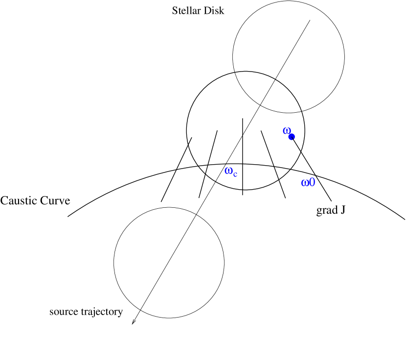
Figure 2: If we consider a large stellar disk, the source line ($\bar{\partial}J$) for each point in the disk can be diverse. Given a source position $\omega$ inside the caustic curve, $\omega_{0}$ will define the source line, and the image line of the two images will be at $z_{\circ}$: $z_{\circ}\mapsto\omega_{0}$ as we have discussed in the text and the caption of Fig.1. One issue is how well we can recover the images $z_{\pm}$ and their amplification $\sqrt{(4\delta\omega_{-}J_{-})^{-1}}$ when we take a nearby but arbitrary caustic point $\omega_{c}$ as the origin where the coordinate system $\{E_{+},E_{-}\}$ is defined and the power series expansion coefficients are calculated.

References

- Chang (1984) Chang, K. 1984, A & A 130, 157
- Chang & Refsdal (1979) Chang, K., and Refsdal, S. 1979, Nature, 282, 561
- Gaudi & Petters (2001) Gaudi, S., and Petters, A. 2001, astro-ph/0112531
- Rhie (1997) Rhie, S. H. 1997, ApJ, 484, 63
- Rhie (2001) Rhie, S. H. 2001, astro-ph/0103463
- Rhie & Bennett (2001) Rhie, S. H., and Bennett, D. P. 2001, “Notes on Gravitational Binary Lenses” (unpublished)
- Rhie & Bennett (1999) Rhie, S. H., and Bennett, D. P. 1999 (rb99), astro-ph/9912050
- Schneider, Ehlers, & Falco (1992) Schneider, P., Elhers, J., and Falco, E. 1992 (SEF), “Gravitational Lenses”, Springer-Verlag