An Untriggered Search for Optical Bursts

Abstract

We present an untriggered search for optical bursts with the ROTSE-I telephoto array. Observations were taken which monitor an effective 256 square degree field continuously over 125 hours to $m_{ROTSE}=15.7$. The uniquely large field, moderate limiting magnitude and fast cadence of $\sim$10 minutes permits transient searches in a new region of sensitivity. Our search reveals no candidate events. To quantify this result, we simulate potential optical bursts with peak magnitude, $m_{p}$, at t=10 s, which fade as $f=\left(\frac{t}{t_{0}}\right)^{\alpha_{t}}$, where $\alpha_{t}<0$. Simple estimates based on observational evidence indicate that a search of this sensitivity begins to probe the possible region occupied by GRB orphan afterglows. Our observing protocol and image sensitivity result in a broad region of high detection efficiency for light curves to the bright and slowly varying side of a boundary running from $[\alpha_{t},m_{p}]=[-2.0,6.0]$ to $[-0.3,13.2]$. Within this region, the integrated rate of brief optical bursts is less than $1.1\times 10^{-8}~{}{\rm s}^{-1}~{}{\rm deg}^{-2}$. At $\sim$22 times the observed GRB rate from BATSE, this suggests a limit on $\frac{\theta_{opt}}{\theta_{\gamma}}\lesssim 5$ where $\theta_{opt}$ and $\theta_{\gamma}$ are the optical and gamma-ray collimation angles, respectively. Several effects might explain the absence of optical bursts, and a search of the kind described here but more sensitive by about 4 magnitudes should offer a more definitive probe.

Motivation

Gamma-ray bursts remain one of the great mysteries in astrophysics. Although there have been some concrete measurements of the energetics of some bursts through redshift determination (eg. Metzger et al. (1997), Kulkarni et al. (1998)), there is little firm knowledge of how the energy is produced. In fact, the total production is still uncertain by approximately 2 or 3 orders of magnitude because of the unknown level of postulated collimated jets. Additionally, despite recent advances in multi-wavelength detection strategies, the total number of GRBs studied optically remains small. While various observations have placed the internal-external shock scenario on a relatively firm footing (eg. Akerlof et al. (1999), Sari and Piran (1999)) for some bursts, it is not verified for most. Bright optical bursts are the expected signature of reverse external shocks, but have been ruled out for several gamma-ray bursts Akerlof et al. (2000), Kehoe et al. (2001), Park et al. (1999), which argues against a uniform behavior.

Gamma-ray bursts are believed to emit synchrotron or inverse Compton radiation from material moving at ultra-relativistic velocities. The resultant strong Lorentz beaming of the emission will decrease as the shocked material slows down. If the ultra-relativistic bulk flow is a collimated jet, radiation at wavelengths longer than gamma rays, believed to be produced by this slower material, will be emitted through a larger solid angle Rhoads (1998). This suggests a population of orphan optical bursts with timescales similar to GRBs, but more frequent and with no gamma-ray signature.

With the unfortunate demise of the Compton Gamma-Ray Observatory, the rate of GRB detections overall has decreased dramatically. The physics of jets may prove valuable in the ongoing effort to observe multiwavelength emission from their progenitors and in a wider variety of conditions than studied so far. Conversely, the study of the relative rates of gamma-ray and “orphan” optical bursts may uniquely probe the open question of collimation. Whether useful constraints can be obtained in this way is currently the subject of some debate, some holding the view that strong limits are possible from such a measurement (eg. Rhoads (1998)). On the other hand, Dalal et al. (2002) have asserted these efforts are unable to measure the collimation angle. However, in Dalal et al. (2002) only very late, slow cadence, and narrow-field searches were discussed. In addition, the estimates of optical lightcurves are based heavily on an interpretation of a model which has yet to be confirmed for GRB’s.

Observational evidence for bursts at longer wavelengths than gamma-rays is at present very sketchy. One search for the expected higher rate of X-ray afterglows has been performed Grindlay (1999) with negative results. On the other hand, mysterious optical transients have been observed in deep, narrow-field searches (eg. Tyson et al. (2001)). Although selected based on spectral criteria rather than photometric (lightcurve) critera as in our paper, the SNe optical search of vanden Berk et al. (2001) has recently revealed a new type of AGN at 17th magnitude exhibiting characteristics reminiscent of GRB optical afterglows. This is close to the ROTSE-I detection threshold, and as a background Gal-Yam et al. (2002) will have to be understood for any GRB orphans search.

A substantial complication to these kinds of searches arises from the fact that the rates of rapidly varying optical transients are poorly understood. Study of eruptive variables with timescales of variation of order $\sim$1h has been limited to searches with very non-uniform sky coverage. The catalog of known rapidly eclipsing and pulsating systems has a similar limitation. The rates of burst-like AGN activity, such as from SDSS J124602.54+011318.8, are also very poorly understood. Aside from being interesting in their own right, these transients are sources of background for GRB optical counterpart searches, whether triggered or untriggered.

Method

For all of these reasons, we have devised an optical burst search strategy based almost solely on considerations taken directly from data. Enough GRB late optical afterglows have been measured to indicate that lightcurves of the form $f=\left(\frac{t}{t_{0}}\right)^{\alpha_{t}}$, with $\alpha_{t}\sim-1$, are typical. When extrapolated back to times nearer the burst phase, the observed afterglow lightcurve of GRB 970228, which is fairly typical of those observed so far, indicates emission brighter than 16th magnitude for the first 30 minutes. While the non-detections of optical bursts imply this is not the typical scenario Kehoe et al. (2001), Akerlof et al. (2000), Park et al. (1999), the observed optical burst from GRB 990123 was actually brighter than this extrapolation would indicate. This sensitivity is attainable in 3 minute exposures with ROTSE-I Kehoe et al. (2001), and it places the observation of an optical burst lightcurve brighter than this limit over 30 minutes just within the telescope’s capability. We therefore take this lightcurve signature as our fundamental search criterion.

Because this search is limited by field area covered and integrated observation time, it makes sense to maximize both in our study. The hypothesized 30 minute window of detectibility for ROTSE-I sets the number of different pointings we can accomplish while we expect an optical burst to be visible which, in turn, sets the cadence of our observations. We will discuss this more in the Observations section, but ROTSE-I can accomplish 2 pointings in the allotted time. In general, for a rapidly fading lightcurve, the cadence of a wide-field search must increase with decreasing aperture. This permits fewer pointings by the smaller telescope but this is compensated for by the larger field of view. Despite the modest sensitivity of ROTSE-I, we are aided by its relatively large etendue, $D^{2}\Omega$, a measure of sensitivity for such searches. This product varies relatively little over a wide range of instruments because the useful solid angle for fixed focal plane area decreases as $D^{-2}$ as the aperture, $D$, increases. Thus, under the assumptions made in this paper, ROTSE-I is roughly equivalent to a 0.5m, f/1.8 system. At the BATSE fluence sensitivity of $10^{-8}$ to $10^{-7}~{}{\rm ergs}/~{}{\rm cm}^{2}$, there are approximately two bursts per $4\pi$ steradians per day. If the optical emission fills a cone 5 times wider than that for the gamma-rays, then a detectable optical burst potentially occurs once per 160 hours in a single ROTSE-I field of 256 square degrees.

The uniquely large field and fast cadence of the observations taken for this analysis push transient searches in a very different part of observational phase space than have been pursued before. To both tune our search strategy and estimate our sensitivity to the sought after signature, we have employed a simple Monte Carlo simulation. This simulation has three main functions: (1) reproduce the photometric behavior of ROTSE-I measurements, (2) explore our search efficiency for a range of input optical burst lightcurve parameters, and (3) quantify the search sensitivity given the observing protocols and limiting magnitudes of the actual data taken. We ignore in this simulation model dependent assumptions about relativistic beaming or spectral evolution so that our result can be interpreted as generally as possible. We will describe this simulation more in the Analysis section.

Observations

Our search for optical bursts utilizes data taken with the ROTSE-I telephoto array Kehoe et al. (2001), which consists of four telescopes arranged in a $2\times 2$ configuration, each with an 8 degree field of view and 14” pixels. The major challenge in our analysis is the successful rejection of $\sim$$1.5\times 10^{5}$ non-variable sources for over 2000 observations in each pointing, as well as suppression of astrophysical transients and instrumental backgrounds. At a bare minimum, any candidate for an optical burst must be well-detected in at least two observations. This stipulation, in conjunction with the 30 minute window constraint, largely dictates our observational approach.

We have taken the data used in this analysis in two main pointing modes, stare and switch. The first mode consists of repeated images of a single field each night with no repointings to other locations. This stare data was acquired in two different periods. In mid-December of 1999, two separate fields were monitored on different days, while in mid-April, we covered another field extensively, originally to monitor the X-ray nova XTE J1118+480 Wren et al. (2001). Camera ‘d’ was not operational during half of these observing nights, and camera ‘c’ was inoperable on one. The total stare data set comprises an effective monitoring of 256 square degrees in 80 s exposures for 47.5 hours. The observation dates and coordinates for these fields, and the total area covered, are given in Table 1.

While the stare data provides excellent temporal coverage of any transients which may occur, the field-of-view probed during our crucial 30 minute window is unduly restricted. As mentioned above, the finite visibility window of the hypothesized optical bursts dictates that we maximize the area covered in the allotted time. With ROTSE-I, we can fit two pointings into this timeframe. We employ a protocol in which five 80 s exposures are taken at each pointing, followed by a repointing at a second location where another five exposures are taken. The telescope then returns to the first field and restarts. This leaves blocks of five 80 s exposures with 7 minute gaps for each of the two pointings. One peculiarity of this switch mode occurs when we co-add pairs of images later – namely, each cycle has an un-coadded fifth image. This extra image alternates between preceding or following the two co-adds. We have chosen two of our standard sky patrol fields which pass through the zenith during the late summer and which have a galactic latitude greater then 20 degrees to avoid Galactic extinction and overcrowding. The data were taken from late August through early October 2000 during periods chosen to avoid bright moonlight (see Table 1).

For the observations presented in this analysis we instituted a dithering observing procedure to suppress backgrounds stationary on the CCD. This involved a Z-shaped rastering by about 2.5’ on a side ($\sim$10 pixels) during the observing sequence to relocate bad pixels in celestial coordinates in consecutive frames.

Data Reduction

Reduction of the raw images taken for this study involves an initial calibration of the images, through a co-addition and recalibration phase, to lightcurve construction. This analysis generated 14,000 raw images which were processed to approximately 8000 epochs and $2.5\times 10^{8}$ photometric measurements. The backgrounds and processing time incurred necessitated data reduction as the images were taken, while adding the ability to diagnose and, if possible, correct for various issues of image quality.

The initial calibration of raw images is described in Kehoe et al. (2001) and involves three main steps: correction of images, source extraction, and astrometric and photometric calibration. Images are corrected through the subtraction of dark current and flat-fielding. The darks, flats and bad pixel lists are generated at the beginning of the three major periods of data collection. The corrected images are analyzed using SExtractor Bertin and Arnouts (1996) to produce object catalogs. To speed up processing, we have optimized the choice of clustering parameters while not significantly degrading the ability to extract sources in crowded environments. When an object aperture contains a bad pixel, we flag the object in that observation as bad. The photometric and astrometric calibration involves matching the resultant list of sources to the Hipparchos catalog Høg et al. (1998). As will be described in the Analysis section, our search depends on the statistical study of lightcurve data. For our final calculated search efficiencies to be correct, we must reproduce the observed photometric fluctuations seen in actual ROTSE-I data. We find that an irreducible 0.01 mag fluctuation, in addition to the normal statistical one, reproduces the observed behavior well. We assign this as the minimum systematic error for all observations.

Final Image Processing

Once the astrometry for each frame is established, we can co-add images in pairs to improve our sensitivity. We do this instead of taking exposures of twice the length to increase the dynamic range available in our 14-bit CCDs, to help suppress bad pixel and other instrumental backgrounds, and to permit a later augmentation of the search at twice the temporal granularity. For each field per night (ie. 4 for stare, 8 for switch), we independently number frames starting at ‘1’ for the first image. We co-add each even numbered frame to its immediately preceding odd numbered frame if it is adjacent in time. The even numbered frame is mapped to the odd numbered frame using a bilinear interpolation of pixel intensities to best avoid position resolution degradation and image artifact creation. During the co-addition, intensities of known bad pixels in the first and second images are replaced with the median of their 8 neighbors and are given zero weight. Pixels in the final co-added image with weight $<$ 2.0 are rescaled to homogenize the image. Since the first and second images are dithered with respect to each other, bad pixel locations generally have correct image data from one of the two images. As a further precaution, once the final co-added image is itself clustered and calibrated as described above, found objects are flagged if a bad pixel falls within their 5 pixel wide aperture. Typical image sensitivities of $m_{ROTSE}=15.7$ were obtained for co-added images.

The next step of the processing chain involves removing images which exhibit instrumental problems. Images must satisfy a $5\sigma$ limiting magnitude of at least 14.75, regardless of whether they are co-adds. This generally removes epochs from early or late in a night which are affected by twilight, although it also rejects images taken when weather is not of good observation quality. The position resolution of an image must also be less than 0.15 pixel ($\sim$2 arcsec). This removes images which did not co-add well, due usually to some large obstruction (eg. a tree late in the evening as the field moves towards the horizon) or rare slipping of the mount clutch which compromises the astrometric warp map.

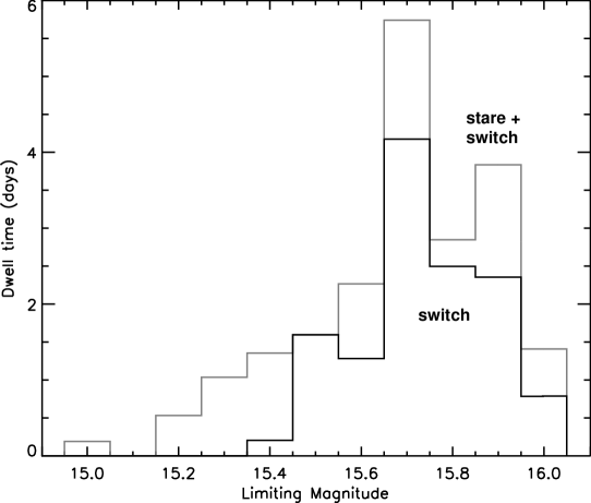
Figure 1: Distribution of integrated observing times vs. limiting magnitude for the 64 square degree field of a single camera. The limiting magnitudes range from 15.0 to 16.1 for the stare data, and 15.4 to 16.1 for the switch data. The total observing time for this size field is 20.8 days.

The last step before lightcurve construction involves the elimination from the data sample of epochs or whole nights exhibiting instrumental problems. For nights with $N$ operational cameras, we omit epochs when fewer than $N-1$ cameras are taking observation quality images. We require whole nights to have at least two contiguous hours of images that pass quality cuts, where contiguous means that no two consecutive epochs are missing. The surviving nights generally exhibit very stable quality over those observations we included. To quantify our observations, we calculate for each good night the median limiting magnitude of the images used, and the total observing time. These are indicated in Figure 1.

Lightcurve Construction

For each camera, the good object lists for each night are matched to provide lightcurves for all detected sources. We remove any object which is not seen in at least one consecutive pair of observations, while we retain all isolated observations of objects passing this selection. To avoid suspect photometry, intermittent sources arising from deblending fluctuations, or moving objects, we flag a source’s observations when the measured position is more than one half pixel from the mean source location.

After we have created a filtered list of calibrated lightcurves, we must perform an internal correction to remove systematic photometric mismeasurements due to such difficulties as the presence of thin haze over a portion of a frame, or increased vignetting due to a sticking shutter. More serious problems occur when power-lines or trees cross an image or when shutters obstruct a portion of an image. In each of these cases, we determine either a small relative photometric correction and systematic error, or in more extreme situations flags to indicate the problem and exclude the image area. We begin by selecting a set of good template sources in each matched list. For each source to enter this list, we count those observations which have good photometry. If these criteria are satisfied for more than 75% of the epochs in which the source location was imaged, the object becomes a template source and we calculate its median magnitude in good observations. Each image is then divided into 100 pixel square subtiles, and photometric offsets for each template source having statistical error less than 0.1 mag in these subtiles are calculated. The number of template sources, $n_{i}$, within a typical subtile, $i$, is around 50. A relative photometry map is then calculated to be the median of these offsets, $o_{i}$, for each subtile. The standard deviation of the offsets, $\sigma_{o,i}$, which for good subtiles is typically around 0.03 magnitudes, is used to calculate a systematic error $\varepsilon_{i}$ on $o_{i}$. In addition, subtiles are classified as bad if $n_{i}<5$, or if $\sigma_{o,i}>0.1$ magnitude. These selections remove obstructions and large photometric gradients due to out-of-focus foreground objects, which constituted approximately 2% of the data sample. Each observation of each object is then corrected by the $o_{i}$ using a bilinear interpolation, and the $\varepsilon_{i}$ is added in quadrature to that observation’s systematic error. If the subtile is flagged as bad, then the object’s observations are likewise flagged.

The lightcurve analysis proceeds from those observations of a particular source which pass basic quality cuts. The source must neither be saturated, nor near an image boundary. The aperture magnitude must be properly measured. The position of the source in good observations must be less than 0.5 pixels from the source’s mean coordinates. The inefficiency incurred for these selections is negligible. There must also be no known bad pixels within the source aperture, and the subtile containing the source must have a well-measured photometric offset. The former inefficiency is approximately 10%, while the latter is 2% as stated earlier.

Analysis

Lightcurve Selection

Based on our observationally motivated model, we look for lightcurves which may have timescales for the brightest optical emission which is similar to the gamma-ray emission of a GRB. In addition, we may expect a decaying lightcurve with $\alpha_{t}<0$. This signature is unlike any other known type of optical transient, and our lightcurve selection exploits this. We begin by cutting on simple statistical variables designed to efficiently identify a fast-rising transient with a power-law decay, while removing backgrounds. These backgrounds come in two kinds. The first originate from astrophysical processes such as low amplitude pulsating and eclipsing systems, irregular fast variables, flare stars, and asteroids. The second kind is dominated by various instrumental transients like those resulting from unregistered bad pixels, poor photometry, or moderate mount clutch failures not identified by our image quality cuts.

In order to obtain an a priori selection, we first studied the instrumental background by performing a grid search on the April 9th stare data of camera ‘b’ ($2\%$ of the total search sample) in terms of the maximum variation amplitude, $\Delta$, and the significance of that variation, $\sigma_{\Delta}$. We took as comparison the 13 eclipsing and pulsating systems we observe in this sample down to variation amplitudes of approximately 0.1 magnitude. We explored the region of $\Delta=[0.1..0.25]$ and $\sigma_{\Delta}=[2.0..5.0]$, and we selected cuts of $\Delta>0.1$ and $\sigma_{\Delta}>5.0$ which minimized the total background while retaining substantial efficiency for real, low amplitude variables.

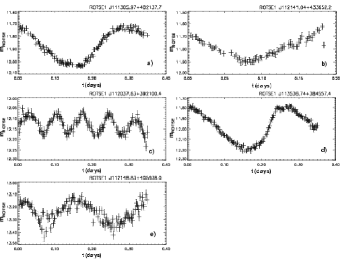
Figure 2: Five single-night lightcurves for candidate pulsating variables from the April 2000 stare data. None of these are previously identified as variable. Observations indicated are good observations after relative photometry. Errors are stat. $+$ sys.

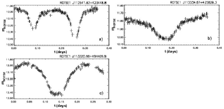
Figure 3: Three lightcurves for candidate eclipsing binary variables from the April 2000 stare data. Only ROTSE1 J112541.62+423448.8 was previously known to be variable. Observations indicated are good observations after relative photometry. Errors are stat. $+$ sys.

These variables generally come in two main types: pulsating stars such as the five indicated in Figure 2, and eclipsing systems such as the three illustrated in Figure 3. Of these 8 variables, only one is previously identified as such: the Algol binary BS UMa (ie. ROTSE1 J112541.62+423448.8) Skiff (1999). The rest are low amplitude variables difficult to identify in photographic plates. ROTSE1 J112037.63+392100.4 and ROTSE1 J113536.74+384557.4 may be a $\delta$ Scu and an RRc, respectively, but we have not fully classified the variables in this sample at this time. However, averaging over four fields, we estimate the rate for variables with amplitude $>0.1$ mag and period $<1$d to be of order $0.1{\rm deg}^{-2}$ for eclipsing systems and $0.2{\rm deg}^{-2}$ for pulsating systems. Several variables with longer timescale variation (ie. $~{}0.7-3$ d) are also observed, and the approximate rate of these is $0.2{\rm deg}^{-2}$. Note that the data is out of the galactic plane.

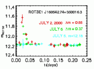
Figure 4: A candidate flare star from the July 2000 test switch data. Observations indicated are good observations after relative photometry. Errors are stat. $+$ sys. Two outbursts were observed 4 days apart with amplitudes of approximately 0.5 mag and durations of about 30 min. The rest of the lightcurve, including the intermediate day July 5, show the source at a constant 12.18 m. The lightcurves are arbitrarily aligned to peak at the same time.

We further investigated the instrumental background behavior in switch data taken in July, 2000. These fields are not included in the search due to a substantial worsening of the problem with the tracking of the mount. This was later almost completely fixed, greatly reducing the background in subsequent switch data. The remaining backgrounds largely consisted of very stable sources with one anomalous photometric measurement. Cutting on a $\chi^{2}$ calculated from observations not including the most significant variation, $\chi_{c}^{2}$, was effective against these. A candidate flare-star, ROTSE1 J160542.74+350016.3, was observed in outburst twice in this July data as shown in Figure 4.

We examined the effect of this selection on our hypothesized optical burst signal. We simulated the expected GRB signature with a simple Monte Carlo generating a variety of lightcurves with no emission during the first 10 s, and then peaking at $m_{p}$ from 6.0 to 15.0. A power-law fading with $\alpha_{t}$ from -0.05 through -3.0 followed thereafter. A cut of $\chi_{c}^{2}>3.0$ is very efficient for the simulated bursts and removes most backgrounds passing our other cuts. Note that the calculation of $\chi_{c}^{2}$ requires an object be seen in at least three good observations. This in turn means our search will be insensitive to variations lasting less than about 7 minutes. All of the simulated optical bursts passing our $\chi_{c}^{2}$ cut also had a $\Delta>0.5$ magnitude. We tighten our selection accordingly to remove most of the remaining low amplitude periodic variables seen in the data background samples. Thus our lightcurve cuts require an overall significant variation with $\Delta>0.5$ and $\sigma_{\Delta}>5.0$, and substantial variability in the rest of the lightcurve with $\chi_{c}^{2}>3.0$. Although designed with a simple power-law time decay in mind, these cuts are efficient for a wide range of optical burst lightcurves.

At this stage, our candidate sample was dominated by three major sources of background. The first consisted largely of bright, moderate amplitude pulsating and eclipsing systems, most of which have not yet been cataloged. The second category consisted of non-varying sources present in most observations but poorly measured in more than one observation. For the most part, these latter are not flare stars. These categories of candidate are easily measured on other nights and so rejected. Given the results of our simulated lightcurves, these are highly unlikely to correspond to GRB optical counterparts. The last category arises from the fact that the outer region of each camera field has relative photometry corrections which start to break down where interpolation becomes extrapolation. We discard these regions in our search, and we thereby incur a 2.5% inefficiency.

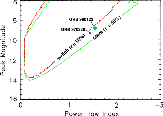
Figure 5: Sensitive region for observing protocols. The red outline delineates 50% efficiency for switch data, while the green outline indicates the stare data 50% efficiency. The efficiency turn-on for a particular limiting magnitude is quite steep. Both are calculated for co-add image sensitivies of 15.7. The increased efficiency in stare data for steeply decaying lightcurves is indicated. The locations of GRB 970228, extrapolated from afterglow data Galama et al. (2000), and GRB 990123 Akerlof et al. (1999) are shown for comparison.

Figure 5 indicates, for a co-add sensitivity of 15.7 magnitude, the 50% efficiency contour for our simulated bursts after our final lightcurve cuts. GRB 970228 and GRB 990123 are shown for comparison. We see that the selection is efficient for simulated bursts in a particular subset of the $m_{p}$ vs. $\alpha_{t}$ parameter space. The boundary of this region is relatively sharp, and moves vertically as a night’s typical image sensitivities increase. The increased sensitivity to steep lightcurves with the stare protocol results from the uninterrupted nature of the observing.

Search Results

After the selection mentioned in the previous section, 50 candidate lightcurves remain. Twenty six of these candidates are located along a CCD column in camera ‘c’ with improper charge transfer and so rejected. Hand-scanning and comparison to images without candidates revealed that 12 of the remaining 24 lightcurves were due to bad pixels. On three nights (000824, 000903, 000906), there was an intermittent 15% increase in the number of hot pixels observed in data. The reason for this behavior is not understood. Although it affects a small portion of image real-estate, these pixels were not properly dark-subtracted, flagged or removed in co-addition. One set of candidates happens when two bad pixels are near enough that they land on the same $\alpha$, $\delta$ in consecutive frames. The other candidates consist of a hot pixel landing between two nearby bright stars, overlapping a star or stars just below reliable detection, or following a satellite trail in the next image.

Ten of the remaining 12 candidates are within 15” ($\sim$1 pixel) of objects in the USNO A2.0 catalog USNO (1998) brighter than 17th mag. in $R$. By rejecting these, we incur an inefficiency dominated by the loss of the image region contained in $\sim 6$ pixel area around all of the USNO source positions. Since the largest occupancy per camera is about 50,000 stars, this cut incurs a 7% inefficiency.

The last two candidates clearly move slowly in our images. These match the expected coordinates of the asteroids (1719) Jens and (17274) 2000 LC16, and we reject them. Thus, we find no optical bursts in this study.

Our data sample was taken at several different sensitivities and both stare and switch pointing modes, and this will alter the sensitivity of our search from that shown in Figure 5. Using the simple Monte Carlo already described, we generated over 20 million bursts folding in the fractions with co-add sensitivities and pointing mode given in Figure 1. A region of $[\alpha_{t},m_{p}]$ parameter space is efficiently accepted which lies on the bright and long side of a rough line between [-2.0,6.0] and [-0.3,13.2]. This result is shown in Figure 6. A final additional inefficiency of 20% for our selection comes from three main sources: bad pixel removal ($\varepsilon=0.9$), bad image regions ($\varepsilon=0.98$), removal of previously known sources ($\varepsilon=0.93$), and removal of field edges ($\varepsilon=0.975$).

Discussion

We have performed the most extensive untriggered search for optical bursts in wide-field data to date. After study of $1331.4~{}{\rm deg}^{2}~{}{\rm days}$, we find no candidates down to a typical limiting sensitivity of $m_{ROTSE}=15.7$. This sensitivity is of the order necessary to study the potential rates for optical bursts from GRBs based on simple beaming hypotheses. At a maximum efficiency of 80%, we accept transients which are brighter and longer than a boundary running from $[\alpha_{t},m_{p}]=[-2.0,6.0]$ to $[-0.3,13.2]$. In this region, we therefore rule out an integrated optical burst rate greater than $1.1\times 10^{-8}~{}{\rm s}^{-1}~{}{\rm deg}^{-2}$. At a rate ten times greater, we reject bursts bounded by $[\alpha_{t},m_{p}]=[-2.6,6.0]$ to $[-0.3,14.3]$.

As there is no empirical information about the optical properties of orphan afterglows, any interpretation of this result in the context of GRB beaming is uncertain. If we consider that the optical emission is collimated into some jet angle, $\theta_{opt}$, which may be different than the gamma-ray collimation angle, $\theta_{\gamma}$, then the relative rate of gamma-ray to optical bursts may indicate something about the relative magnitudes of these angles. Compared to the observed GRB rate from BATSE of $5\times 10^{-10}~{}{\rm s}^{-1}~{}{\rm deg}^{-2}$, our limit on optical burst rates translates into a limit on $\frac{\theta_{opt}}{\theta_{\gamma}}\lesssim 5$.

This result seems to conflict with the much higher rates predicted in the analysis of Frail et al. (2001). There may be several reasons for this. We have assumed that all of the bursts observed by BATSE would have produced optical bursts of sufficient intensity to be observed above 16th magnitude. The relationship of optical emission during this early phase to gamma-ray emission is not known well enough to rigorously justify this assumption. In this case, however, a search of the kind described in this analysis but deeper by 2-4 magnitudes should provide a more incisive probe, given the distribution of GRB fluences relative to those we have discussed in this paper.

Although most GRBs with both X-ray and radio afterglows seem to have optical counterparts, it is still possible that obscuration at the source is dimming a large number of the optical bursts we would otherwise see. For instance, there is evidence for as much as 5 mag extinction for GRB 970828 Groot et al. (1998). Ultimately, the question of extinction at the source is still tied up with the identity of the progenitor. In collapsar models Woosley (1993), substantial extinctions could result.

Lastly, we have ignored the specifics of how the changing Lorentz factor of the burst ejecta affects the very early optical emission. This behavior is complex, and very model dependent, but for very off-axis viewing the observed optical flux is likely to peak later, and at a lower value (eg. Granot et al. (2002)), than might be suggested by extrapolating back from the late afterglow. Observationally, many optical afterglows have exhibited breaks in their lightcurves which may indicate analogous behavior for nearly on-axis viewing Frail et al. (2001). In a couple of cases, the early lightcurve exhibits a time decay index of $\sim-0.8$ (Stanek et al. (1999), Stanek et al. (2001)) which puts them in a relatively sensitive region of Figure 6. Any optical burst with such a slope and brighter than about 12th mag at it’s peak would have been observed, and bursts with peak brightnesses of $\sim 13$th mag would be detected with lower efficiency. As one moves more off-axis, the slope at early times becomes shallower until eventually it may rise to the break point. The suppression of this early emission will result in a decreased ability to observe these bursts. However, it should be kept in mind that, regardless of when the peak occurs relative to the initial event, our search will be sensitive to these lightcurves if the emission is brighter than 16th mag in a way similar to the optical bursts we have simulated (ie. detection in at least three images with overal $\Delta>0.5$). In any case, a limiting magnitude deeper by $\sim$ 4 mag would substantially improve the chances for detection, especially in light of observed GRB optical afterglow brightnesses.

This search technique can be improved and extended in several ways. The main source of background was instrumental. To consider much larger numbers of observations, it is important to reduce the number of bad pixels and shutter malfunctions, and avoid visual obstructions. Another improvement would be to increase the sophistication of the relative photometry calibration. Most importantly, the next step for an untriggered optical burst search would be to consider deeper fields, such as available with the ROTSE-III 0.5m telescopes. This kind of search will likely be looking for more gradual optical variation than sought in this paper. For robust identification, it may be necessary to obtain spectral verification of candidate orphans which are more likely to be found at the sensitivity of R0TSE-III. The search must be made immune to the kind of background engendered in SDSS J124602.54+011318.8, in particular.

This analysis has implications for our ability to extend our GRB studies. We have already used the techniques described here to search for optical counterparts for several archival BATSE triggered bursts Kehoe et al. (2001). In addition, they are a crucial step towards our goal of near real-time detection with the ROTSE-III telescopes the optical transients associated with GRB triggers from satellite-based gamma-ray observations.

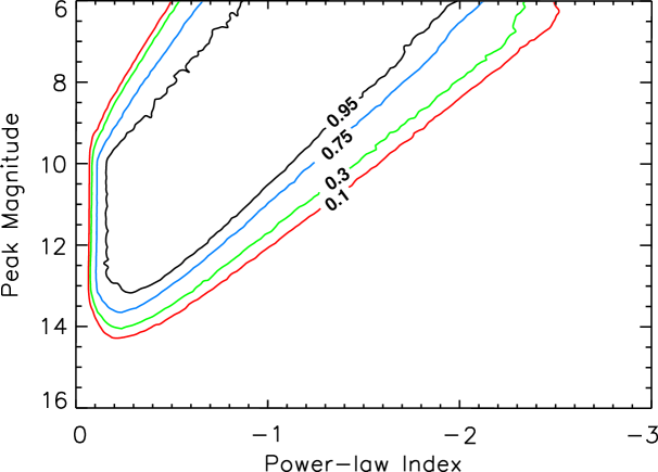
Figure 6: Cumulative sensitivity to simulated sources of given $m_{p}$ and $\alpha_{t}$. Contours are generated by folding the observing time as given in Figure 1 with the protocol efficiency contours such as given in Figure 5. Contours giving the 95%, 75%, 30% and 10% efficiency levels are specified. The gradient in efficiency is primarily due to the varying protocol and limiting magnitudes of the ROTSE-I observations. The efficiencies are given relative to a rate of $1.1\times 10^{-8}~{}{\rm s}^{-1}~{}{\rm deg}^{-2}$.

year and month	dates	$\alpha$	$\delta$	$\Omega(deg^{2})$	dwell-time $\times$ area	pointing mode
Dec, 1999	16	4h	+15∘	768	$4.355\times 10^{6}{\rm deg}^{2}{\rm s}$	stare
	17	5h24m	+11.4∘	512		stare
Apr, 2000	9,10,13,14	11h42m	+44∘	768	$3.9375\times 10^{7}{\rm deg}^{2}{\rm s}$	stare
	15-17			(1024)
Aug, 2000	24,25,31	0h	+30∘	1024	$4.2799\times 10^{7}{\rm deg}^{2}{\rm s}$	switch
Sep, 2000	1-3,5,6,28,29
Oct, 2000	1-4,6
Aug, 2000	24,25,31	23h	+15∘	1024	$2.8488\times 10^{7}{\rm deg}^{2}{\rm s}$	switch
Sep, 2000	1-3,5,6,29
Oct, 2000	1-4

Table 1: Itemization of observation properties. The coordinates of fields and total area covered are given, as well as the dates and observing protocol for each.

References

- Akerlof et al. (1999) Akerlof, C., et al. 1999, Nature, 398, 400
- Akerlof et al. (2000) Akerlof, C., et al. 2000, ApJ, 532, L25-L28
- Bertin and Arnouts (1996) Bertin, E., and Arnouts, S. 1996, A&AS, 117, 393
- Dalal et al. (2002) Dalal, N., Greist, K. and Pruet, J., 2002, ApJ, 564, L209-L215
- Frail et al. (2001) Frail, D. A., et al., 2001. ApJ, 562, L55-L58
- Galama et al. (2000) Galama, T. J., et al. 2000, ApJ, 536, 185
- Gal-Yam et al. (2002) Gal-Yam, A. 2002, subm. PASP, astro-ph/0202354
- Granot et al. (2002) Granot, J. et al. 2002, ApJ, 568, 820-829.
- Grindlay (1999) Grindlay, J. E., 1999, ApJ, 510, 710-714.
- Groot et al. (1998) Groot, P. et al. 1998, ApJ, 493, L27-L30.
- Høg et al. (1998) Høg, E., Kuzmin, A., Bastian, U., Fabricius, C., Kuimov, K., Lindegren, L., Makarov, V., and Roser, S. 1998, A&A, 335, L65.
- Skiff (1999) Skiff, B. A., 1999. IAU Inform. Bullet. Var. Stars, 4720, 1-8.
- Kehoe et al. (2001) Kehoe, R., et al., 2001, in Supernovae and Gamma-Ray Bursts: The Greatest Explosions since the Big Bang, ed. M. Livio, N. Panagia, and K. Sahu (Cambridge: Cambridge Univ. Press), 47
- Kehoe et al. (2001) Kehoe, R., et al., 2001, ApJ, 554, L159-L162
- Kulkarni et al. (1998) Kulkarni, S., et al. 1998, Nature, 393, 35
- Metzger et al. (1997) Metzger, M. R., Cohen, J. G., Chaffee, F. H., & Blandford, R. D. 1997, IAU Circ. 6676
- Park et al. (1999) Park, H. S., et al. 1999, A&AS, 138, 577
- Rhoads (1998) Rhoads, J., 1998, in Gamma-Ray Bursts: 4th Huntsville Symposium, ed. C. Meegan, R. Preece, and T. Koshut (AIP), 699
- Sari and Piran (1999) Sari, R. and Piran, T. 1999, ApJ, 517(2), L109-L112
- Stanek et al. (1999) Stanek, K. Z. et al. 1999, ApJ, 522, L39-L42.
- Stanek et al. (2001) Stanek, K. Z. et al. 2001, ApJ, 563, 592-596.
- Tyson et al. (2001) Tyson, T. et al., 2001, http://dls.bell-labs.com/transients.html
- USNO (1998) USNO A-2.0 catalog, http://www.nofs.navy.mil/.
- vanden Berk et al. (2001) vanden Berk, D., Lee, B. C. et al., 2001. subm. to ApJ, astro-ph/0111054
- Woosley (1993) Woosley, S. 1993, ApJ, 405, 273
- Wren et al. (2001) Wren, J., et al., 2001. ApJ, 557, L97-L100