Adiabatic oscillations of non–rotating superfluid neutron stars

We present results concerning the linear (radial and non–radial) oscillations of non–rotating superfluid neutron stars in Newtonian physics. We use a simple two–fluid model to describe the superfluid neutron star, where one fluid consists of the superfluid neutrons, while the second fluid contains all the comoving constituents (protons, electrons). The two fluids are assumed to be “free” in the sense of absence of vortex–mediated forces like mutual friction or pinning, but they can be coupled by the equation of state, in particular by entrainment. We calculate numerically the eigen-frequencies and -modes of adiabatic oscillations, neglecting beta–reactions that would lead to dissipation. We find a doubling of all acoustic–type modes (f–modes, p–modes), and confirm the absence of g–modes in these superfluid models. We show analytically and numerically that only in the case of non–stratified background models (i.e. with no composition gradient) can these doublets of acoustic modes be separated into two distinct families, which are characterised by either co– or counter–moving fluids respectively, and which are sometimes referred to as “ordinary”- and “superfluid” modes. In the general, stratified case, however, this separation is not possible, and these acoustic modes can not be classified as being either purely “ordinary” or “superfluid”. We show how the properties of the two–fluid modes change as functions of the coupling by entrainment. We find avoided mode-crossings for the stratified models, while the crossings are not avoided in the non–stratified, separable case. The oscillations of normal-fluid neutron stars are recovered as a special case simply by locking the two fluids together. In this effective one–fluid case we find the usual singlet f– and p–modes, and we also find the expected g–modes of stratified neutron star models.

1 Introduction

The study of stellar oscillations has proved very fruitful in improving our understanding of the inner structure and dynamics of stars (the terms helio– and astro–seismology have been coined), for which the oscillation modes can often be observed rather directly. The best developed example of this probing of the internal structure of an astrophysical body via its oscillations is probably the Earth. In the case of neutron stars, the observation of oscillations is unfortunately not possible in such a direct way, and has not yet been achieved. In practically all cases we can only observe the regular radio–pulses of neutron stars, which are virtually unaffected by its oscillations and give information mostly about their rotation rate. Nevertheless this field bears great potential interest: on one hand the better understanding of neutron star oscillations could eventually help to elucidate the phenomenon of glitches, which is probably the most striking and puzzling aspect of observed neutron star dynamics. This phenomenon still represents somewhat of a mystery, even though the crucial role of superfluidity seems well established (see Link et al. (2000); Carter et al. (2000) for recent discussions). On the other hand, several highly sensitive gravitational wave detectors are expected to reach their full sensitivity within the next few years, and neutron star oscillations represent one of the potentially most interesting sources of gravitational waves. Gravitational wave detection could open a new and complementary observational window onto neutron stars, which would allow us to learn much more about their inner structure and dynamics than it is currently possible with the purely electro-magnetic observations.

Currently most studies of neutron star oscillations are based on simple perfect fluid models, which neglects the crucial importance of superfluidity in neutron stars. The presence of substantial amounts of superfluid matter in neutron stars is backed by a number of theoretical calculations of the state of matter at these extreme densities (e.g. see Baldo et al. (1992); Sjöberg (1976)), and by the qualitative success of superfluid models to accommodate observed features of glitches and their relaxation.

The first study to point out the importance of superfluidity for the oscillation properties of neutron stars was by Epstein (1988), who has argued in a local (sound wave) analysis that superfluidity should lead to new modes and modify the previously known modes. Lindblom & Mendell (1994) have argued further for the existence of these modes, but failed to find them numerically. Lee (1995) presented the first numerical results indicating the presence of new modes that did not exist in perfect fluid models, and the absence of g–modes which would have been present in the non–superfluid case. A local analysis by Andersson & Comer (2001a) has given further analytic evidence for the absence of g–modes in simple superfluid models. The relativistic numerical analysis by Comer et al. (1999) has shown an effective doubling of acoustic modes in superfluid models with respect to the normal fluid case. Recently this work has been extended by Andersson et al. (2002) to include entrainment, and they have shown that avoided mode crossings occur when one varies the entrainment parameter. The relevance of superfluid oscillations for gravitational wave detection has been discussed by Andersson & Comer (2001b). Some studies have also started to look at oscillations of rotating superfluid neutron stars (Lindblom & Mendell 2000) and Sedrakian & Wasserman (2000).

Despite the number of studies on oscillations of non–rotating superfluid neutrons stars, we think that this problem still deserves attention and that several points needed to be clarified. In particular it is worth emphasising the importance of stratification for the nature of superfluid oscillations, a point that has not yet been fully appreciated. We demonstrate here that only in non–stratified models can the eigenmode spectrum be separated into two families of modes, one of which is identical to the case of a normal–fluid star, while the other is characterised by counter–motion of the two fluids and vanishing gravitational perturbation. These two distinct families are usually referred to as “ordinary” and “superfluid” modes. Stratification of the background star, however, couples these distinct mode-families and renders them non–separable. As a consequence every mode shares qualitative properties of both families to some extent, and the resulting mode spectrum consists of modes that bear no direct connection to the normal fluid case. The two–fluid model used here to describe superfluid neutron stars is practically equivalent to those use in previous studies, and we refer the reader to Andersson & Comer (2001a) and Prix et al. (2002) for a more extensive discussion about its physical motivations and justification.

The plan of this paper is as follows: in Sect. 2 we introduce the basic equations for the general two–fluid neutron star model, and in Sect. 3 we develop its linear perturbation equations and show how to recover the special case of a single perfect fluid. In Sect. 4 we specialise to the simpler case of adiabatic oscillations of free, cold fluids, and we derive the necessary boundary conditions. In this section we also show that the separation into two distinct mode families is possible only for non–stratified models. Sect. 5 presents the numerical results concerning the background models, the eigenmode spectrum and its dependence on entrainment (resulting in avoided crossings), as well as the one–fluid results where we recover the expected composition g–modes. We present our conclusions and a discussion of necessary future work in Sect. 6.

2 The general two–fluid neutron star model

2.1 The general two–fluid equations

The equations and notation for the Newtonian two–fluid neutron star model used here are based on a more general formalism described in Prix (2002), which is the Newtonian analogue of a generally relativistic framework developed by Carter (1989). In this section we will briefly summarise the general model and equations relevant for the present work, and we refer the reader to Prix (2002) for the derivation and more detailed discussion of this model.

We describe a neutron star as a system consisting of two fluids: a superfluid of neutrons, and a normal fluid of comoving constituents, which include protons, electrons and entropy (and generally further particles like muons etc). We denote the particle number densities for neutrons, protons and electrons as $n_{\rm n}$, $n_{\rm p}$ and $n_{\rm e}$ respectively, and we use $s$ for the entropy density. The velocities of the two fluids are $\@vec{v}_{\rm n}$ for the neutron fluid, and $\@vec{v}_{\rm c}$ for the fluid of comoving constituents, the relative velocity $\@vec{\Delta}$ between the two fluids is therefore

$$\@vec{\Delta}\equiv\@vec{v}_{\rm c}-\@vec{v}_{\rm n}\,.$$ (1)

On the local (“mesoscopic”) level, a superfluid is constrained to be in a state of irrotational flow, and its angular momentum will be accommodated by a lattice of “microscopic” vortices. However, for the global description of a neutron star we are more interested in a “macroscopic” description of the superfluid, obtained by averaging over volume elements containing a large number of vortices, but which are small compared to the dimensions of the neutron star. In this macroscopic description, the superfluid has a continuous vorticity and nearly behaves like an ordinary fluid (apart from small anisotropies due to the vortex-tension, which we will neglect). The absence of (local) viscosity still allows the superfluid to move relative to the normal fluid, but the presence of the vortex lattice now allows for a direct force between the two fluids. In the case of this force being zero, the vortex lattice moves with the superfluid and we refer to this situation as free fluids. If the vortices are “locked” to the normal fluid (e.g. as can happen in the crust), the mutual force will be non-zero but strictly non–dissipative. This is known as “vortex pinning”. Only in the intermediate cases, where a friction force causes the vortices to have a different velocity from both the normal fluid and the superfluid, energy is dissipated. In this case the mutual force is usually referred to as “mutual friction”.

An essential simplification of the present two–fluid model is that we neglect all electrodynamic effects, as we assume the charge densities of protons and electrons to be strictly balanced, i.e.

$$n_{\rm e}=n_{\rm p}\,.$$ (2)

Therefore we can effectively eliminate the electrons from our description, as their density and velocity is entirely specified by the protons.

We note that in “transfusive” models (as first set up in Langlois et al. (1998)), i.e. models which allow for $\beta$–reactions (${\rm n}\rightleftharpoons{\rm p}+{\rm e}+\bar{\nu}$) between the two fluids, the total mass in the reaction has to be conserved in a consistent Newtonian description. Therefore we set

$$m_{\mathrm{b}}\equiv m_{\rm n}\equiv m_{\rm p}+m_{\rm e}\,.$$ (3)

The respective mass densities of the two fluids can now be written as

$$\rho_{\rm n}=m_{\mathrm{b}}n_{\rm n}\,,{\quad\text{and}\quad}\rho_{\rm c}=m_{\mathrm{b}}n_{\rm p}\,,$$ (4)

and the total mass density $\rho$ is simply $\rho=\rho_{\rm n}+\rho_{\rm c}$.

The (local) kinematics of the system is completely described (up to arbitrary rotations and boosts) in terms of $\rho_{\rm n}$, $\rho_{\rm c}$, $s$ and $\Delta^{2}$. The dynamics is determined by the internal energy density function ${\cal E}$ or equation of state, which is a function of the form ${\cal E}={\cal E}(s,\rho_{\rm n},\rho_{\rm c},\Delta^{2})$. This energy function defines the first law of thermodynamics for this system by its total differential, namely

$$d{\cal E}=T\,ds+\widetilde{\mu}^{\rm c}\,d\rho_{\rm c}+\widetilde{\mu}^{\rm n}\,d\rho_{\rm n}+\alpha\,d\Delta^{2}\,.$$ (5)

This differential defines the dynamic quantities, namely the temperature $T$, the specific chemical potentials $\widetilde{\mu}^{\rm c}$, $\widetilde{\mu}^{\rm n}$, and the entrainment $\alpha$ as the thermodynamic conjugates of the kinematic quantities $s$, $\rho_{\rm c}$, $\rho_{\rm n}$ and $\Delta$. The specific chemical potentials $\widetilde{\mu}$ are related to the more common definition of the chemical potentials $\mu$ via $\widetilde{\mu}\equiv\mu/m_{\mathrm{b}}$. We note that $\mu^{\rm c}$ is not simply the proton chemical potential, because adding a proton in this model implies adding an electron as well (due to (2)), and therefore one can see that $\mu^{\rm c}=\mu^{\rm p}+\mu^{\rm e}$, where $\mu^{\rm p}$ and $\mu^{\rm e}$ are the respective proton and electron chemical potentials.

The function $\alpha$ defined in (5) reflects the dependence of the internal energy on the relative velocity $\Delta$ between the two fluids, which characterises the so–called entrainment effect. This entrainment function $\alpha$ has dimensions of a mass density, and it will be useful in the following to define the two dimensionless entrainment functions $\varepsilon_{\rm n}$ and $\varepsilon_{\rm c}$ as

$$\varepsilon_{\rm c}\equiv{2\alpha\over\rho_{\rm c}}\,,{\quad\text{and}\quad}\varepsilon_{\rm n}\equiv{2\alpha\over\rho_{\rm n}}={\rho_{\rm c}\over\rho_{\rm n}}\varepsilon_{\rm c}\,.$$ (6)

The “generalised” pressure $P$ is introduced as the Legendre-conjugate of the energy density, namely by the usual thermodynamic relation

$${\cal E}+P=\rho_{\rm n}\widetilde{\mu}^{\rm n}+\rho_{\rm c}\widetilde{\mu}^{\rm c}+sT\,,$$ (7)

which results in the total differential of the pressure function $P(\widetilde{\mu}^{\rm c},\widetilde{\mu}^{\rm n},T,\Delta^{2})$:

$$dP=\rho_{\rm n}\,d\widetilde{\mu}^{\rm n}+\rho_{\rm n}\,d\widetilde{\mu}^{\rm c}+s\,dT-\alpha\,d\Delta^{2}\,.$$ (8)

This generalised pressure $P$ can be seen to reduce to the usual definition of the pressure of a perfect fluid in the case of $\Delta=0$.

The equations of motion of this two–fluid system are derived from a “convective” variational principle in Prix (2002), and here we only present the resulting equations. The conservation of energy results in the following equation:

$$T\mathit{\Gamma}_{\rm s}=\@vec{f}\cdot\@vec{\Delta}+\beta\mathit{\Gamma}_{\rm n}\,,$$ (9)

where $\mathit{\Gamma}_{\rm s}$ and $\mathit{\Gamma}_{\rm n}$ are the creation rates of entropy and neutrons respectively, i.e.

$$\mathit{\Gamma}_{\rm s}\equiv\partial_{t}s+\@vec{\nabla}\cdot(s\@vec{v}_{\rm c})\,,\;\;\text{and}\;\;\mathit{\Gamma}_{\rm n}\equiv\partial_{t}\rho_{\rm n}+\@vec{\nabla}\cdot(\rho_{\rm n}\@vec{v}_{\rm n})\,,$$ (10)

while the proton creation rate $\mathit{\Gamma}_{\rm c}$ has to satisfy $\mathit{\Gamma}_{\rm c}=-\mathit{\Gamma}_{\rm n}$ for baryon conservation. The quantity $\beta$ in (9) characterises the deviation from chemical equilibrium and its explicit expression if found as

$$\beta\equiv\widetilde{\mu}^{\rm c}-\widetilde{\mu}^{\rm n}-{1\over 2}\left(1-2\varepsilon_{\rm n}\right)\,{\Delta^{2}}\,.$$ (11)

This is the Newtonian analogue of a result first found in the relativistic transfusive model by Langlois et al. (1998). We note that there is an additional kinetic term with respect to the naive $\widetilde{\mu}^{\rm c}-\widetilde{\mu}^{\rm n}$ in the case of relative motion. The mutual force density $\@vec{f}$ (the sign convention is such that this force acts on the neutron fluid) is a direct interaction force between the two fluids, which in the case of a superfluid stems from vortex interactions like pinning or mutual friction. In order to ensure explicitly that the second law of thermodynamics, i.e. $\mathit{\Gamma}_{\rm s}\geq 0$, is satisfied by (9), we can write the neutron creation rate $\mathit{\Gamma}_{\rm n}$ and the mutual force $\@vec{f}$ in the form

$$\mathit{\Gamma}_{\rm n} = \Xi\beta\,,\hskip 48.36958pt\quad\text{with}\quad\Xi\geq 0\,,$$ (12)

$$\@vec{f} = \eta\@vec{\Delta}+\@vec{\kappa}\times\@vec{\Delta}\,,\quad\text{with}\quad\eta\geq 0\,,$$ (13)

where the non–negative functions $\Xi$ and $\eta$ govern the beta–reaction rate and the friction force, while the vector $\@vec{\kappa}$ allows for a non–dissipative Magnus–type force (i.e. orthogonal to the relative motion). A non–transfusive model, i.e. one that does not allow for beta reactions ${\rm n}\rightleftharpoons{\rm c}$, has $\Xi=0$, and free vortices correspond to $\eta=0$ and $\@vec{\kappa}=0$, while pinned vortices correspond to $\eta=0$ and $\@vec{\kappa}\not=0$.

The momentum equation for the superfluid neutrons is given by

$$(\partial_{t}+\@vec{v}_{\rm n}\cdot\@vec{\nabla})(\@vec{v}_{\rm n}+\varepsilon_{\rm n}\@vec{\Delta})+\@vec{\nabla}(\widetilde{\mu}^{\rm n}+\Phi)+\varepsilon_{\rm n}\Delta_{a}\@vec{\nabla}v_{\rm n}^{a}={1\over\rho_{\rm n}}\@vec{f},\quad$$ (14)

while the equation for the normal fluid reads as

$$(\partial_{t}+\@vec{v}_{\rm c}\cdot\@vec{\nabla})(\@vec{v}_{\rm c}-\varepsilon_{\rm c}\@vec{\Delta})+\@vec{\nabla}(\widetilde{\mu}^{\rm c}+\Phi)-\varepsilon_{\rm c}\Delta_{a}\@vec{\nabla}v_{\rm c}^{a}\quad$$

$$+{s\over\rho_{\rm c}}\nabla T=-{1\over\rho_{\rm c}}\@vec{f}+\left(1-\varepsilon_{\rm c}-\varepsilon_{\rm n}\right){\mathit{\Gamma}_{\rm n}\over\rho_{\rm c}}\@vec{\Delta}\,.$$ (15)

The gravitational potential $\Phi$ is related to the mass densities $\rho_{\rm n}$ and $\rho_{\rm c}$ via the Poisson equation

$$\nabla^{2}\Phi=4\pi G(\rho_{\rm n}+\rho_{\rm c})\,.$$ (16)

2.2 The static equilibrium background

We consider a static background star, so we set

$$\@vec{v}_{\rm n}=\@vec{v}_{\rm p}=\@vec{\Delta}=0\,,{\quad\text{and}\quad}\mathit{\Gamma}_{\rm n}=\mathit{\Gamma}_{\rm c}=\mathit{\Gamma}_{\rm s}=0\,,$$ (17)

which by (13) implies the vanishing of the mutual force, i.e. $\@vec{f}=0$. Because chemical reactions would not be negligible on long timescales, we also assume the background star to be in chemical equilibrium, i.e.

$$\beta=\widetilde{\mu}^{\rm c}-\widetilde{\mu}^{\rm n}=0\,.$$ (18)

These equilibrium conditions reduce the equation of motion (14) to

$$\@vec{\nabla}\widetilde{\mu}^{\rm n}=\@vec{\nabla}\widetilde{\mu}^{\rm c}=-\@vec{\nabla}\Phi\,,$$ (19)

and with (15) this also implies that the background star is in thermal equilibrium, i.e. $\@vec{\nabla}T=0$.

The static background has to be spherically symmetric, and therefore (19) and (16) lead to the following equation for the background:

$$\widetilde{\mu}^{\prime\prime}(r)+{2\over r}\widetilde{\mu}^{\prime}(r)=-4\pi G\rho(r)\,,$$ (20)

where we have introduced the equilibrium chemical potential $\widetilde{\mu}\equiv\widetilde{\mu}^{\rm n}=\widetilde{\mu}^{\rm c}$, and the prime (^′) denotes the radial derivative $d/dr$.

The equation of state allows one to relate the equilibrium chemical potential $\widetilde{\mu}$ directly to the total mass density $\rho$ at constant temperature, and therefore the background is fully determined. The numerical method for solving this equation will be discussed in sect. 5.

In the following it will be convenient to use the radius $R$ and central density $\rho_{0}$ of the static background as basis units for length and mass density, so the corresponding “natural unit” for frequencies is $\sqrt{4\pi G\rho_{0}}$. All equations in the following are expressed in these natural units except otherwise stated.

2.3 Entrainment and effective masses

For small relative velocities $\Delta$, we can separate the “bulk” equation of state from the entrainment by expanding ${\cal E}(s,\rho_{\rm n},\rho_{\rm c};\Delta^{2})$ in terms of $\Delta$, i.e. by writing

$${\cal E}={\cal E}^{(0)}(s,\rho_{\rm n},\rho_{c})+\alpha^{(0)}(s,\rho_{\rm n},\rho_{\rm c})\Delta^{2}+{\cal O}(\Delta^{4})\,,$$ (21)

where the quantities ${\cal E}^{(0)}$ and $\alpha^{(0)}$ are evaluated at zero relative velocity $\Delta$. The background equation of state ${\cal E}^{(0)}$ is therefore decoupled from the entrainment function $\alpha^{(0)}$, and we can specify these two functions independently. The link between the entrainment function $\alpha$ and the equivalent description in terms of effective masses $m^{*}$ (Andreev & Bashkin 1975) has been discussed in previous work (Prix et al. 2002), and it can be shown that one can express $\alpha$ in terms of the proton effective mass $m_{\rm p}^{*}$ (which is generally a function of the densities), in the form

$$2\alpha=\rho_{\rm c}\left(1-{m_{\rm p}^{*}\over m_{\mathrm{b}}}\right)\,.$$ (22)

The dimensionless entrainment functions $\varepsilon_{\rm n}$ and $\varepsilon_{\rm c}$ can then be expressed according to (6) as

$$\varepsilon_{\rm c}=1-{m_{\rm p}^{*}\over m_{\mathrm{b}}}\,,{\quad\text{and}\quad}\varepsilon_{\rm n}={\rho_{\rm c}\over\rho_{\rm n}}\,\varepsilon_{\rm c}\,.$$ (23)

3 Linearised perturbation equations

3.1 Oscillations of superfluid neutron stars

We consider small perturbations with respect to the static equilibrium background described in Sect. 2.2. Linearising the equations of motion (14) and (15) yields

$$\rho_{\rm n}\partial_{t}(\delta\@vec{v}_{\rm n}+\varepsilon_{\rm n}\,\delta\@vec{\Delta})+\rho_{\rm n}\@vec{\nabla}(\delta\widetilde{\mu}^{\rm n}+\delta\Phi)=\delta\@vec{f}\,,\qquad\qquad\quad\mbox{}$$ (24)

$$\rho_{\rm c}\partial_{t}(\delta\@vec{v}_{\rm c}-\varepsilon_{\rm c}\,\delta\@vec{\Delta})+\rho_{\rm c}\@vec{\nabla}(\delta\widetilde{\mu}^{\rm c}+\delta\Phi)=-\delta\@vec{f}-s\@vec{\nabla}\delta T,\quad\mbox{}$$ (25)

where $\delta Q$ denotes the Eulerian perturbation of the quantity $Q$. The perturbation of the mutual force (13) is given by

$$\delta\@vec{f}=\eta\delta\@vec{\Delta}+\@vec{\kappa}\times\delta\@vec{\Delta}\,,$$ (26)

and the linearised energy conservation (9) and (12) together with the condition of baryon conservation lead to

$$\partial_{t}\,\delta s+\@vec{\nabla}\cdot(s\,\delta\@vec{v}_{\rm c}) = 0\,,$$ (27)

$$\partial_{t}\,\delta\rho_{\rm n}+\@vec{\nabla}\cdot(\rho_{\rm n}\,\delta\@vec{v}_{\rm n}) = \;\;\;\Xi\,(\delta\widetilde{\mu}^{\rm c}-\delta\widetilde{\mu}^{\rm n})\,,$$ (28)

$$\partial_{t}\,\delta\rho_{\rm c}+\@vec{\nabla}\cdot(\rho_{\rm c}\,\delta\@vec{v}_{\rm c}) = -\Xi\,(\delta\widetilde{\mu}^{\rm c}-\delta\widetilde{\mu}^{\rm n})\,.$$ (29)

The perturbed Poisson equation (16) reads (in natural units) as

$$\nabla^{2}\delta\Phi=\delta\rho_{\rm n}+\delta\rho_{\rm c}\,.$$ (30)

The system is closed by specification of the mutual force functions $\eta$ and $\@vec{\kappa}$, the transfusion function $\Xi$, and an equation of state which allows to express the dynamical quantities $\delta T$, $\delta\widetilde{\mu}^{\rm n}$ and $\delta\widetilde{\mu}^{\rm c}$ in terms of the kinematic variables $\delta s$, $\delta\rho_{\rm n}$ and $\delta\rho_{\rm c}$, thereby reducing the number of unknown perturbation quantities to $13$, which corresponds exactly to the number of equations.

3.2 The special case of normal–fluid neutron stars

It is interesting to compare the superfluid neutron star case with the normal fluid case, where the two constituents $n$ and ${\rm c}$ are moving together and form a single perfect fluid. This case is obviously just a subclass of the two–fluid case discussed so far, namely subject to the additional constraint $\@vec{v}_{\rm n}=\@vec{v}_{\rm c}$, and therefore

$$\delta\@vec{v}_{\rm n}=\delta\@vec{v}_{\rm c}=\delta\@vec{v}\,,\quad{\quad\Longrightarrow\quad}\delta\@vec{\Delta}=0\,.$$ (31)

By linking the two constituents together, the degrees of freedom have been reduced by three, and instead of the individual momentum equations (24) and (25), now only the sum of momenta can be required to be conserved, i.e.

$$\rho\,\left(\partial_{t}\delta\@vec{v}+\@vec{\nabla}\delta\Phi\right)+\rho_{\rm n}\@vec{\nabla}\delta\widetilde{\mu}^{\rm n}+\rho_{\rm c}\@vec{\nabla}\delta\widetilde{\mu}^{\rm c}+s\@vec{\nabla}\delta T=0\,.$$ (32)

We introduce the notation

$$\rho_{\rm c}=x_{\rm c}\rho\,,\quad\rho_{\rm n}=x_{\rm n}\rho\,,{\quad\text{and}\quad}s=\widetilde{s}\rho\,,$$ (33)

for the proton and neutron fractions $x_{\rm c}$ and $x_{\rm n}$, and the specific entropy $\widetilde{s}$, which allows us to rewrite the one–fluid equation of motion (32) in the slightly more familiar form

$$\partial_{t}\delta\@vec{v}+\@vec{\nabla}\left({\delta P\over\rho}+\delta\Phi\right)-\left[\delta\beta\,\@vec{\nabla}x_{\rm c}+\delta T\,\@vec{\nabla}\widetilde{s}\right]=0\,,$$ (34)

where we used the fact that the total pressure differential $dP$ of (8) in this perfect fluid case reduces to

$$dP=\rho_{\rm n}\,d\widetilde{\mu}^{\rm n}+\rho_{\rm n}\,d\widetilde{\mu}^{\rm c}+s\,dT\,.$$ (35)

We can now compare (32) to the standard expression for the Euler equation of stellar oscillations of non–rotating stars (Cox 1980; Unno et al. 1989), which is usually written as

$$\partial_{t}\delta\@vec{v}+\@vec{\nabla}\left({\delta P\over\rho}+\delta\Phi\right)+{\cal C}(r)\,(\@vec{\nabla}\cdot\delta\@vec{v})\,\@vec{A}=0\,,$$ (36)

where ${\cal C}(r)$ is a function of the background, and $\@vec{A}$ is the so–called Schwarzschild discriminant that is responsible for presence of g–modes. By comparing eqs. (32) and (34), we see that $\@vec{A}$ will be non–zero (indicating the presence of g–modes) whenever $\@vec{\nabla}\widetilde{s}\not=0$ or $\@vec{\nabla}x_{\rm c}\not=0$. This reflects the well–known fact that any type of stratification, either in specific entropy $\widetilde{s}$ or in the chemical composition $x_{\rm c}$, will result in g–modes, as pointed out by Reisenegger & Goldreich (1992).

4 Adiabatic oscillations of ”free”, cold fluids

4.1 Reduction to a 1D eigenvalue problem

In order to close the system of perturbation equations (24)–(30), we need specific models for the mutual force $\@vec{f}$, the transfusion $\Xi$, in addition to an equation of state of the form ${\cal E}(\rho_{n},\rho_{\rm c},{\rm s})$, all of which are highly dependent on microphysical models and are rather poorly known at the present stage. For this reason, we will postpone the inclusion of these effects to future work, and focus on the case of purely adiabatic oscillations (i.e. $\Xi=0$) of free fluids (meaning $\@vec{f}=0$). We will further neglect temperature effects (which is generally a very good approximation except for very young neutron stars), so we set $s=0$ and $T=0$. The resulting simplified system of equations is

$$\partial_{t}\delta\rho_{\rm n}+\@vec{\nabla}\cdot\left(\rho_{\rm n}\,\delta\@vec{v}_{\rm n}\right) = 0\,,$$ (37)

$$\partial_{t}\delta\rho_{\rm c}+\@vec{\nabla}\cdot\left(\rho_{\rm c}\,\delta\@vec{v}_{\rm c}\right) = 0\,,$$ (38)

$$\partial_{t}\left[(1-\varepsilon_{\rm n})\,\delta\@vec{v}_{\rm n}+\varepsilon_{\rm n}\delta\@vec{v}_{\rm c}\right] = -\@vec{\nabla}\left(\delta\widetilde{\mu}^{\rm n}+\delta\Phi\right)\,,$$ (39)

$$\partial_{t}\left[(1-\varepsilon_{\rm c})\,\delta\@vec{v}_{\rm c}+\varepsilon_{\rm c}\delta\@vec{v}_{\rm n}\right] = -\@vec{\nabla}\left(\delta\widetilde{\mu}^{\rm c}+\delta\Phi\right)\,,$$ (40)

$$\nabla^{2}\delta\Phi = \delta\rho_{\rm n}+\delta\rho_{\rm c},.$$ (41)

We point out that this system of equations is identical to the one used in Andersson & Comer (2001a), which was obtained from a Newtonian limit of the relativistic equations. It is also related to the equations of Lindblom & Mendell (1994), which are expressed in the “orthodox” formulation of superfluids (Landau & Lifshitz 1959), while the present description is based on the “canonical” approach introduced by Carter (1989).

Using the equation of state we can link the density perturbations $\delta\rho_{\rm X}$ to $\delta\widetilde{\mu}^{\rm X}$ (with the constituent index notation ${\rm X}={\rm n},\,{\rm c}$) to linear order, namely

$$\begin{array}[]{r l}\delta\rho_{\rm n}=&{\cal S}_{{\rm n}{\rm n}}\,\delta\widetilde{\mu}^{\rm n}+{\cal S}_{{\rm n}{\rm c}}\,\delta\widetilde{\mu}^{\rm c}\,,\\ \delta\rho_{\rm c}=&{\cal S}_{{\rm c}{\rm n}}\,\delta\widetilde{\mu}^{\rm n}+{\cal S}_{{\rm c}{\rm c}}\,\delta\widetilde{\mu}^{\rm c}\,,\\ \end{array}$$ (42)

where the symmetric “structure matrix” ${\cal S}_{{\rm X}{\rm Y}}$ is defined as

$$\left({\cal S}^{-1}\right)_{{\rm X}{\rm Y}}\equiv{\partial\widetilde{\mu}^{\rm X}\over\partial\rho_{\rm Y}}={\partial^{2}{\cal E}\over\partial\rho_{\rm X}\,\partial\rho_{\rm Y}}\,,\qquad{\rm X},{\rm Y}\in\{{\rm n},{\rm c}\}\,.$$ (43)

Due to the dual role of the pressure $P$ in (7) and (8), we can equivalently express ${\cal S}_{{\rm X}{\rm Y}}$ as

$${\cal S}_{{\rm X}{\rm Y}}={\partial\rho_{\rm X}\over\partial\widetilde{\mu}^{\rm Y}}={\partial^{2}P\over\partial\widetilde{\mu}^{\rm X}\,\partial\widetilde{\mu}^{\rm Y}}\,.$$ (44)

We note that although we have assumed free fluids, i.e. there is no direct force acting between them, the fluids are nevertheless locally coupled by the equation of state; we can distinguish two sources of this coupling, one is due to the non–diagonal term ${\cal S}_{{\rm n}{\rm c}}$ in (42), while the second is due to the entrainment terms $\varepsilon_{\rm X}$.

The background quantities $\widetilde{\mu}^{\rm X}$ can be seen in (19) to behave like the gravitational potential $\Phi$; this means in particular that their gradient is always finite, even at the surface. Therefore $\delta\widetilde{\mu}^{\rm X}$ is finite everywhere, contrary to $\delta\rho_{\rm X}$ which can diverge at the surface when $\rho^{\prime}\rightarrow-\infty$. This is seen from the relation $\Delta\rho=\delta\rho+\xi^{r}\,\rho^{\prime}(r)$ between the Lagrangian perturbation $\Delta\rho$ and the Eulerian $\delta\rho$, for a radial displacement $\xi^{r}$. On physical grounds $\Delta\rho$ must be bounded everywhere (as it reflects the physical property of a fluid element), while the first–order Eulerian quantity $\delta\rho$ diverges at the surface whenever $\rho^{\prime}\rightarrow-\infty$ and $\xi^{r}\not=0$ at $r=R$. This might seem problematic for the validity of the equations, but it only reflects the fact that in this case even an infinitesimal displacement of the surface will lead to a finite (as opposed to infinitesimal) Eulerian density change there. By considering Lagrangian instead of Eulerian variables, it can be shown that the physical solution is still well behaved even if $\delta\rho\rightarrow\infty$ at the surface. In this case the first–order quantity $\delta\rho$ no longer approximates the physical Eulerian density change, but the divergence is such that the Lagrangian first–order quantity $\Delta\rho$ is still perfectly regular. If one wanted to impose that $\delta\rho$ should be bounded everywhere (as did Lindblom & Mendell (1994)), then this situation would be inverted and the Lagrangian quantity $\Delta\rho$ would diverge, which is unphysical indeed.

From a numerical point of view it seemed better to solve directly for the well-behaved $\delta\widetilde{\mu}^{\rm X}$ instead of the potentially diverging $\delta\rho_{\rm X}$, by using (42) to substitute for $\delta\rho_{\rm X}$. We note that the coefficients ${\cal S}_{{\rm X}{\rm Y}}$ in this expression will generally diverge (or vanish) at the surface, depending on the equation of state and reflecting the behaviour of $\delta\rho_{\rm X}$. The system of equations (37-41) for eigenmode solutions of the form $\delta Q(\@vec{x},t)=\delta Q(\@vec{x})\,e^{i\omega t}$ now yields

$$\@vec{\nabla}\cdot(\rho_{\rm n}\delta\@vec{v}_{\rm n}) = -i\omega\left[{\cal S}_{{\rm n}{\rm n}}\delta\widetilde{\mu}^{\rm n}+{\cal S}_{{\rm n}{\rm c}}\delta\widetilde{\mu}^{\rm c}\right]\,,$$ (45)

$$\@vec{\nabla}\cdot(\rho_{\rm c}\delta\@vec{v}_{\rm c}) = -i\omega\left[{\cal S}_{{\rm c}{\rm n}}\delta\widetilde{\mu}^{\rm n}+{\cal S}_{{\rm c}{\rm c}}\delta\widetilde{\mu}^{\rm c}\right]\,,$$ (46)

$$\@vec{\nabla}(\delta\widetilde{\mu}^{\rm n}+\delta\Phi) = -i\omega\left[(1-\varepsilon_{\rm n})\,\delta\@vec{v}_{\rm n}+\varepsilon_{\rm c}\,\delta\@vec{v}_{\rm c}\right]\,,$$ (47)

$$\@vec{\nabla}(\delta\widetilde{\mu}^{\rm c}+\delta\Phi) = -i\omega\left[(1-\varepsilon_{\rm c})\,\delta\@vec{v}_{\rm c}+\varepsilon_{\rm n}\,\delta\@vec{v}_{\rm n}\right]\,,$$ (48)

$$\nabla^{2}\delta\Phi = k_{\rm n}\,\delta\widetilde{\mu}^{\rm n}+k_{\rm c}\,\delta\widetilde{\mu}^{\rm c}\,,$$ (49)

where we have introduced the convenient “structure vector” $k_{\rm X}$, which is defined as

$$k_{\rm X}\equiv\sum_{{\rm Y}={\rm n},{\rm c}}S_{{\rm X}{\rm Y}}\,,\qquad{\rm X}\in\{{\rm n},\,{\rm c}\}\,.$$ (50)

For a spherically symmetric background, we can separate the radial and angular dependence and obtain solutions with definite quantum numbers $l$ and $|m|\leq l$ using the ansatz

$$\delta\Phi(r,\theta,\varphi) = \delta\Phi(r)\,Y_{l}^{m}(\theta,\varphi)\,,$$ (51)

$$\delta\widetilde{\mu}^{\rm X}(r,\theta,\varphi) = \delta\widetilde{\mu}^{\rm X}(r)\,Y_{l}^{m}(\theta,\varphi)\,,$$ (52)

$$\delta\@vec{v}_{\rm X}(r,\theta,\varphi) = {W_{\rm X}(r)\over r}\@vec{R}_{l}^{m}+V_{\rm X}(r)\@vec{S}_{l}^{m}-iU_{\rm X}(r)\@vec{T}_{l}^{m},$$ (53)

where the spherical harmonics $Y_{l}^{m}(\theta,\varphi)$ are the eigenfunctions of $r^{2}\nabla^{2}Y_{l}^{m}=-l(l+1)\,Y_{l}^{m}$, and $\@vec{R}$, $\@vec{S}$ and $\@vec{T}$ form the orthogonal harmonic basis, defined as

$$\@vec{R}_{l}^{m}\equiv Y_{l}^{m}\@vec{\nabla}r\,,\quad\@vec{S}_{l}^{m}\equiv\@vec{\nabla}Y_{l}^{m}\,,\quad\@vec{T}_{l}^{m}\equiv\@vec{\nabla}\times\@vec{R}\,,$$ (54)

see Rieutord (1987) for details. The three–dimensional eigenvalue problem (45)-(49) has now been reduced to the following one–dimensional problem:

$$\left(r\rho_{\rm n}W_{\rm n}\right)^{\prime}-{l(l+1)}\rho_{\rm n}V_{\rm n} = -i\omega r^{2}\left[{\cal S}_{{\rm n}{\rm n}}\delta\widetilde{\mu}^{\rm n}+{\cal S}_{{\rm n}{\rm c}}\delta\widetilde{\mu}^{\rm c}\right],$$ (55)

$$\left(r\rho_{\rm c}W_{\rm c}\right)^{\prime}-{l(l+1)}\rho_{\rm c}V_{\rm c} = -i\omega r^{2}\left[{\cal S}_{{\rm n}{\rm c}}\delta\widetilde{\mu}^{\rm n}+{\cal S}_{{\rm c}{\rm c}}\delta\widetilde{\mu}^{\rm c}\right],$$ (56)

$$-r\left({\delta\widetilde{\mu}^{\rm n}}^{\prime}+\delta\Phi^{\prime}\right) = i\omega\left[(1-\varepsilon_{\rm n})W_{\rm n}+\varepsilon_{\rm n}W_{\rm c})\right],\qquad\mbox{}$$ (57)

$$-r\left({\delta\widetilde{\mu}^{\rm c}}^{\prime}+\delta\Phi^{\prime}\right) = i\omega\left[(1-\varepsilon_{\rm c})W_{\rm c}+\varepsilon_{\rm c}W_{\rm n})\right],$$ (58)

$$-\delta\widetilde{\mu}^{\rm n}-\delta\Phi = i\omega\left[(1-\varepsilon_{\rm n})V_{\rm n}+\varepsilon_{\rm n}V_{\rm c})\right],$$ (59)

$$-\delta\widetilde{\mu}^{\rm c}-\delta\Phi = i\omega\left[(1-\varepsilon_{\rm c})V_{\rm c}+\varepsilon_{\rm c}V_{\rm n})\right],$$ (60)

$$\left(r^{2}\delta\Phi^{\prime}\right)^{\prime}-{l(l+1)}\,\delta\Phi = r^{2}\,(k_{\rm n}\,\delta\widetilde{\mu}^{\rm n}+k_{\rm c}\,\delta\widetilde{\mu}^{\rm c})\,.$$ (61)

The axial velocity component $U_{\rm X}$ is decoupled and corresponds to zero frequency $\omega=0$, therefore all non–zero frequency eigenmodes are purely polar. We note that the horizontal velocity equations (59) and (60) only hold for $l>0$, because $\@vec{S}_{0}^{0}=0$.

4.2 Boundary and regularity conditions

4.2.1 At the center

It can be shown that the representation (51)-(53) of a regular physical quantity requires the following asymptotic behaviour of the radial functions as $r\rightarrow 0$,

$$\delta\widetilde{\mu}^{\rm X}\sim\delta\Phi\sim W_{\rm X}\sim V_{\rm X}\sim{\cal O}(r^{l})\,,\qquad{\rm X}\in\{{\rm n},\,{\rm c}\}\,,$$ (62)

where ${\cal O}(r^{l})$ means of order $r^{l}$ or higher. Another requirement is the regularity of the solution at singular points of the equations. From eqs. (57) and (58) we see that $W_{\rm X}$ must vanish as ${\cal O}(r)$ at the origin, while from eqs. (59) and (60) we can derive the further regularity requirement

$$\left(1+r{\rho_{\rm X}^{\prime}\over\rho_{\rm X}}\right)W_{\rm X}+rW_{\rm X}^{\prime}-l(l+1)V_{\rm X}\sim{\cal O}(r^{2})\,.$$ (63)

Regularity of solutions of Poisson’s equation (61) requires

$$\delta\Phi\sim{\cal O}(r^{2})\,\quad\text{for}\quad l>0\,,$$ (64)

while for radial oscillations ($l=0$) only $\delta\Phi^{\prime}\sim{\cal O}(r)$ is required. These constraints are automatically satisfied by (62) for $l\geq 2$, but they are stronger requirements than (62) in the cases $l=1$ and $l=0$.

4.2.2 At the surface

At the outer surface ($r=R$) we need to ensure the continuity of the gravitational potential $\Phi$, which results (e.g. see Ledoux & Walraven (1958)) in the boundary condition

$$\delta\Phi^{\prime}(R)+{l+1\over R}\delta\Phi(R)=-\xi^{r}\,\rho(R-)\,,$$ (65)

where $\xi^{r}$ is the radial displacement of the surface, and $\rho(R-)$ is the inner limit of $\rho(r)$, i.e. $\rho(R-)=\lim_{r\rightarrow R-}\rho(r)$. In the present work we will only consider stars with vanishing density at the surface i.e. $\rho(r)\rightarrow 0$. The conservation equations (55) and (56) contain a (regular) singularity at the surface $r=R$, because $\rho^{\prime}/\rho$ diverges as $\rho\rightarrow 0$. Therefore we need an additional regularity condition that can be obtained by a Frobenius–type expansion around the surface,i.e. $\widetilde{\mu}=0$. We first rewrite these equations as

$$(rW_{\rm X})^{\prime}-l(l+1)V_{\rm X}=-\left[r{\rho_{\rm X}^{\prime}\over\rho_{\rm X}}W_{\rm X}+i\omega r^{2}{\sum{\cal S}_{{\rm X}{\rm Y}}\delta\widetilde{\mu}^{\rm Y}\over\rho_{\rm X}}\right],\;\;$$ (66)

and using the definition (43) of the matrix ${\cal S}_{{\rm X}{\rm Y}}$ together with the equilibrium condition ${\widetilde{\mu}^{\rm n}}{}^{\prime}=\widetilde{\mu}^{\rm c}{}^{\prime}=\widetilde{\mu}^{\prime}$, we can write

$$\rho_{\rm X}^{\prime}=k_{\rm X}\,\widetilde{\mu}^{\prime}\,,$$ (67)

where $k_{\rm X}$ has been defined in (50). In order to simplify the analysis, we will assume that the equation of state becomes decoupled in the limit of vanishing density, i.e.

$$P(\widetilde{\mu}^{\rm n},\widetilde{\mu}^{\rm c})\sim P_{\rm n}(\widetilde{\mu}^{\rm n})+P_{\rm c}(\widetilde{\mu}^{\rm c})\,,$$ (68)

such that $\rho_{\rm n}\sim\rho_{\rm n}(\widetilde{\mu}^{\rm n})$ and $\rho_{\rm c}\sim\rho_{\rm c}(\widetilde{\mu}^{\rm c})$, and $k_{\rm X}\sim{\cal S}_{{\rm X}{\rm X}}$ in this limit. In this case we can write the asymptotic form of (66) as

$$(rW_{\rm X})^{\prime}-l(l+1)V_{\rm X}=-{{\cal S}_{{\rm X}{\rm X}}\over\rho_{\rm X}}\left[r\widetilde{\mu}^{\prime}W_{\rm X}+i\omega r^{2}\delta\widetilde{\mu}^{\rm X}\right],$$ (69)

where the expression in brackets is regular for $\widetilde{\mu}\rightarrow 0$. The behaviour of ${\cal S}_{{\rm X}{\rm X}}/\rho_{\rm X}$ in this limit can be analysed by writing $\rho_{\rm X}$ in the asymptotic form $\rho_{\rm X}\sim(\widetilde{\mu}^{\rm X})^{\alpha}$ (with positive $\alpha$), which is possible due to the assumed decoupling. Therefore we find ${\cal S}_{{\rm X}{\rm X}}=\partial\rho_{\rm X}/\partial\widetilde{\mu}^{\rm X}\sim\widetilde{\mu}^{\alpha-1}$, and so we have identified the singularity in (69) as

$${{\cal S}_{{\rm X}{\rm X}}\over\rho_{\rm X}}\sim\widetilde{\mu}^{-1}\,.$$ (70)

Regularity of the solution therefore requires the following asymptotic behaviour at the surface:

$$r\widetilde{\mu}^{\prime}W_{\rm X}+i\omega r^{2}\delta\widetilde{\mu}^{\rm X}\sim{\cal O}(\widetilde{\mu})\,,\quad\text{for}\quad{\rm X}\in\{{\rm n},\,{\rm c}\}\,.$$ (71)

4.3 Decoupling “ordinary” and “superfluid” modes?

In this section we discuss a change of variables that has been used in several previous studies of oscillations of superfluid neutron stars (Lindblom & Mendell 1994, 1995, 2000; Sedrakian & Wasserman 2000; Andersson & Comer 2001a), namely

$$\begin{array}[]{r l r l}\delta\@vec{\Delta}\equiv&\delta\@vec{v}_{\rm c}-\delta\@vec{v}_{\rm n}\,,&\delta\beta\equiv&\delta\widetilde{\mu}^{\rm c}-\delta\widetilde{\mu}^{\rm n}\,,\\ \delta\@vec{v}\equiv&x_{\rm c}\,\delta\@vec{v}_{\rm c}+x_{\rm n}\,\delta\@vec{v}_{\rm n}\,,&\delta\widetilde{\mu}\equiv&x_{\rm c}\,\delta\widetilde{\mu}^{\rm c}+x_{\rm n}\,\delta\widetilde{\mu}^{\rm n}\,.\\ \end{array}$$ (72)

This choice of variables is motivated by the intuitive idea that the additional degrees of freedom of a second fluid should allow for two different types of motion, characterised roughly by the two fluids being either “co-moving” or “counter-moving”, and which are sometimes referred to as “ordinary” and “superfluid” modes. By choosing such “adapted” coordinates (72), one might hope to separate, or at least simplify the system of equations, but we will see that this is generally not the case.

Using the relations (42) and the definition (67) of $k_{\rm n}$ and $k_{\rm c}$, and defining $k\equiv k_{\rm n}+k_{\rm c}$, we can express the density perturbations $\delta\rho_{\rm X}$ as

$$\begin{array}[]{r l}\delta\rho_{\rm n}=&k_{\rm n}\delta\widetilde{\mu}+\left({\cal S}_{{\rm n}{\rm c}}-x_{\rm c}k_{\rm n}\right)\delta\beta\,,\\ \delta\rho_{\rm c}=&k_{\rm c}\delta\widetilde{\mu}+\left(-{\cal S}_{{\rm n}{\rm c}}+x_{\rm n}k_{\rm c}\right)\delta\beta\,,\\ \end{array}$$ (73)

and therefore

$$\delta\rho=k\delta\widetilde{\mu}-(x_{\rm c}k_{\rm n}-x_{\rm n}k_{\rm c})\,\delta\beta\,.$$ (74)

In the case of a spherically symmetric background considered here, we can use (67) to express

$$x_{\rm c}k_{\rm n}-x_{\rm n}k_{\rm c}=-k{\rho\over\rho^{\prime}}\,x_{\rm c}^{\prime}\,,$$ (75)

and using these variables and relations, we now rewrite the eigenmode equations (37)–(41) in the form

$$k\,\partial_{t}\delta\widetilde{\mu}+\@vec{\nabla}\cdot(\rho\,\delta\@vec{v}) = -x_{\rm c}^{\prime}\,\left[k{\rho\over\rho^{\prime}}\,\partial_{t}\delta\beta\right]\,,$$ (76)

$$\partial_{t}\delta\@vec{v}+\@vec{\nabla}(\delta\widetilde{\mu}+\delta\Phi) = \;\;\,x_{\rm c}^{\prime}\,\left[\delta\beta\,\@vec{e}^{r}\right]\,,$$ (77)

$$\nabla^{2}\delta\Phi-k\,\delta\widetilde{\mu} = -x_{\rm c}^{\prime}\,\left[k{\rho\over\rho^{\prime}}\,\delta\beta\right]\,,$$ (78)

$${\cal K}\,\partial_{t}\delta\beta+\@vec{\nabla}\cdot\left(\rho x_{\rm n}x_{\rm c}\,\delta\@vec{\Delta}\right) = -x_{\rm c}^{\prime}\left[k{\rho\over\rho^{\prime}}\,\partial_{t}\delta\widetilde{\mu}+\rho\,\delta v^{r}\right]\!,$$ (79)

$$\left(1-{2\alpha\rho\over\rho_{\rm n}\rho_{c}}\right)\partial_{t}{\delta\!\@vec{\Delta}}+\@vec{\nabla}\delta\beta = \;\;0\,,$$ (80)

where $\@vec{e}^{r}$ is the radial basis vector, and we introduced the abbreviation ${\cal K}\equiv x_{\rm c}^{2}k_{\rm n}+x_{\rm n}^{2}k_{\rm c}-{\cal S}_{{\rm n}{\rm c}}$.

We see that the “ordinary”-type of motion ($\delta\widetilde{\mu}$, $\delta\@vec{v}$, $\delta\Phi$) does not decouple from the “superfluid”-type variables ($\delta\@vec{\Delta}$, $\delta\beta$) whenever there is stratification, i.e. when $x_{\rm c}^{\prime}\not=0$ ! This can be understood as follows: while a non–zero relative velocity $\delta\@vec{\Delta}$ can be regarded as a characteristic of a superfluid mode (as opposed to modes in a single fluid), the chemical equilibrium deviation $\delta\beta$ is generally non–zero even for a single (but non–barotropic) fluid. In a stratified fluid, any general adiabatic motion will drive a fluid element out of equilibrium, i.e. $\delta\beta$ nonzero is not characteristic for either “superfluid” or “ordinary” modes (contrary to claims in Lindblom & Mendell (1994, 1995)), it is a general feature of modes in stratified fluids, and therefore the choice of variables (72) does not lead to a decoupling of the system in this case.

However, it is interesting to consider for a moment this special case of a non–stratified background (which probably never applies in real neutron stars). Setting the proton fraction $x_{\rm c}$ to a constant, we can separate the equations into two decoupled sets. One system describes “ordinary” modes, namely

$$k\partial_{t}\delta\widetilde{\mu}+\@vec{\nabla}\cdot(\rho\delta\@vec{v}) = 0\,,$$ (81)

$$\partial_{t}\delta\@vec{v}+\@vec{\nabla}(\delta\widetilde{\mu}+\delta\Phi) = 0\,,$$ (82)

$$\nabla^{2}\delta\Phi-k\,\delta\widetilde{\mu} = 0\,,$$ (83)

which are seen to be independent of the entrainment $\varepsilon$ as well as of the coupling through the “bulk” equation of state, i.e. ${\cal S}_{{\rm n}{\rm c}}$. The second system of equations governs the “superfluid” modes and reads as

$$\left(k-{{\cal S}_{{\rm n}{\rm c}}\over x_{\rm n}x_{\rm c}}\right)\,\partial_{t}\delta\beta+\@vec{\nabla}\cdot(\rho\,\delta\@vec{\Delta}) = 0\,.$$ (84)

$$\left(1-{2\alpha\rho\over\rho_{\rm n}\rho_{\rm c}}\right)\,\partial_{t}\,\delta\@vec{\Delta}+\@vec{\nabla}\delta\beta = 0\,,$$ (85)

We see that contrary to the ordinary modes, the superfluid modes do depend on the coupling through entrainment $\alpha$ and the equation of state, i.e. ${\cal S}_{{\rm n}{\rm c}}$, but they are completely decoupled from the gravitational perturbation $\delta\Phi$, as they leave the total density unchanged, i.e. $\delta\rho=0$.

We have therefore shown that in the non–stratified case there exist two separate families, namely “ordinary” modes $(\delta\@vec{v},\delta\widetilde{\mu},\delta\Phi,0,0)$ and “superfluid” modes $(0,0,0,\delta\@vec{\Delta},\delta\beta)$. One of our numerical models (see next section) has a constant proton fraction $x_{\rm c}$, and we will see the present analysis confirmed by the numerical results for this model. In the general stratified case, however, these two mode families are coupled and such a clearcut separation is not possible.

5 Numerical results

5.1 Equation of state: two–constituent polytropes

We use a simple class of two–constituent equations of state which is very convenient to explore the properties of a two–fluid system, namely the following “generalised polytrope”, defined as

$${\cal E}^{(0)}(\rho_{\rm n},\rho_{\rm c})={\kappa_{\rm n}}\,\rho_{\rm n}^{\gamma_{\rm n}}+{\kappa_{\rm c}}\,\rho_{\rm c}^{\gamma_{\rm c}}$$ (86)

which simply consists of the sum of two ordinary polytropes. For regularity of the chemical potentials (5) in the limit $\rho_{\rm n}\rightarrow 0$ and $\rho_{\rm c}\rightarrow 0$, the polytropic indices must satisfy ${\gamma_{\rm n}}\geq 1$ and ${\gamma_{\rm c}}\geq 1$. This equation of state allows the explicit inversion

$$\rho_{\rm n}(\widetilde{\mu}^{\rm n})=\left({\widetilde{\mu}^{\rm n}\over{\kappa_{\rm n}}{\gamma_{\rm n}}}\right)^{N_{\rm n}}\,,\;\;\text{and}\;\;\rho_{\rm c}(\widetilde{\mu}^{\rm c})=\left({\widetilde{\mu}^{\rm c}\over{\kappa_{\rm c}}{\gamma_{\rm c}}}\right)^{N_{\rm c}}\,,$$ (87)

where we have introduced $N_{\rm X}\equiv 1/({\gamma_{\rm X}}-1)$. We see that in chemical equilibrium, i.e. $\widetilde{\mu}^{\rm n}=\widetilde{\mu}^{\rm c}$, the two fluids share a common outer surface. The equilibrium proton fraction $x_{\rm c}$ can be expressed as

$$x_{\rm c}=\left(1+{({\gamma_{\rm c}}{\kappa_{\rm c}})^{N_{\rm c}}\over({\gamma_{\rm n}}{\kappa_{\rm n}})^{N_{\rm n}}}\,\widetilde{\mu}^{N_{\rm n}-N_{\rm c}}\right)^{-1}\,,$$ (88)

which shows that the proton fraction is constant whenever ${\gamma_{\rm n}}={\gamma_{\rm c}}$, while the behaviour in the case of different indices falls into the two categories:

$$0\stackrel{{\scriptstyle\widetilde{\mu}\rightarrow\infty}}{{\longleftarrow}}x_{\rm c}\stackrel{{\scriptstyle\widetilde{\mu}\rightarrow 0}}{{\longrightarrow}}1\,,\quad\text{for}\quad{\gamma_{\rm n}}<{\gamma_{\rm c}}\,,$$ (89)

$$1\stackrel{{\scriptstyle\widetilde{\mu}\rightarrow\infty}}{{\longleftarrow}}x_{\rm c}\stackrel{{\scriptstyle\widetilde{\mu}\rightarrow 0}}{{\longrightarrow}}0\,,\quad\text{for}\quad{\gamma_{\rm n}}>{\gamma_{\rm c}}\,.$$ (90)

5.2 Calculating the background models

The equilibrium background solution is determined by equation (20), together with the regularity requirement $\widetilde{\mu}^{\prime}(0)=0$, and the boundary condition of vanishing pressure at the surface, i.e. $\widetilde{\mu}(1)=0$, where the surface of the static background star is situated at $R=1$ in the natural units defined in Sect. 2.2. Using the equation of state we can express $\rho=\rho(\widetilde{\mu})$ in chemical equilibrium, and therefore equation (20) can be written as the following nonlinear eigenvalue problem,

$$\widetilde{\mu}^{\prime\prime}+{2\over r}\widetilde{\mu}=\lambda\,\rho(\widetilde{\mu})\,,$$ (91)

where the (dimensionless) eigenvalue $\lambda$ is given by

$$\lambda=4\pi G{\rho_{0}\over\widetilde{\mu}(\rho_{0})}R^{2}\,.$$ (92)

The eigenvalue $\lambda$ represents the a–priori unknown radius of the star, and thereby the actual values of our natural units for a given central density $\rho_{0}$. The method used here to solve this equation is to iterate a linear eigenvalue problem that converges to the solution of (91). This can be done by solving in step $k+1$ the following linear eigenvalue problem,

$$\widetilde{\mu}^{\prime\prime}_{k+1}+{2\over r}\widetilde{\mu}^{\prime}_{k+1}=-\lambda_{k+1}\left({\rho(\widetilde{\mu}_{k})\over\widetilde{\mu}_{k}}\right)\,\widetilde{\mu}_{k+1}\,,$$ (93)

where $\widetilde{\mu}_{k}$ is the solution of the of the previous step $k$. The equation in each step is solved using the spectral linear eigenvalue solver package LSB developed by L. Valdettaro and M. Rieutord. With a resolution of 40 Chebychev polynomials and a Gauss–Lobatto collocation method, this iteration converges to about machine precision (i.e. $\sim 10^{-15}$ relative difference between successive steps) in about $20$ steps. Another practical advantage of this method is that we calculate the background quantities on the same Gauss–Lobatto grid we use for the numerical code for the eigenmodes. Even when using a different resolution for the eigenmode–calculation, the Chebychev expansion provides a canonical ${\cal C}^{\infty}$ interpolation which allows us to easily “re-grid” the background solution.

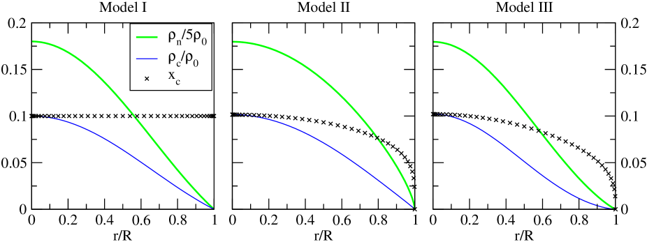
Figure 1: Density profiles and proton fraction $x_{\rm c}$ of the background models I, II and III as defined in table 1. $\rho_{0}$ is the central density. In this figure we have divided the neutron density by 5 in order to obtain similar magnitudes for the different curves.

In principle we can solve the background for any given equation of state, but we restrict our attention in this work to the class of two–constituent polytropes (86).The reason for this choice is their analytic simplicity and because our main emphasis is to clarify the qualitative properties of superfluid neutron stars rather than to construct a physically very precise model. This would in any case be quite impossible in a Newtonian description because of the neglect of relativistic effects, in addition to the important uncertainties in our current knowledge of the equation of state of neutron stars.

In the numerical analysis we consider the three different background models defined in table 1, and which are represented in Fig. 1. These three models correspond to three different types of behaviour at the surface. In the case of Model I one can easily find the background solution analytically, as shown in Prix et al. (2002), which allows us to check the numerical method of calculating the background, and we find a maximal relative error of $10^{-14}$ between the numerical and the analytic solution for model I. Model II represents a generic “stiff” model similar to those used in Comer et al. (1999) and Andersson et al. (2002), which has infinite density gradients at the surface. Model III is of a “soft” type with vanishing density gradients at the surface. These different types of behaviour at the surface are quite analogous to the case of the usual one–constituent polytropes for different polytropic indices.

	${\gamma_{\rm n}}$	${\gamma_{\rm c}}$	${\kappa_{\rm n}}^{a}$	${\kappa_{\rm c}}^{a}$	${\rho_{0}\over\rho_{\mathrm{nuc}}}$	$x_{\rm c}(0)$	${M\over M_{\odot}}$	${R\over\mathrm{km}}$
I	2.0	2.0	0.01	0.09	10.83	0.10	1.414	10.7
II	2.5	2.1	0.01	0.20	3.20	0.10	1.440	14.3
III	1.9	1.7	0.01	0.09	18.65	0.10	1.412	9.4

Table 1: Parameters describing the background models I, II and III, based on the two–constituent polytrope (86). Further shown are the central mass density $\rho_{0}$, the central proton fraction $x_{\rm c}(0)$, the total mass $M$ and the radius $R$. ^a The units of the coefficients $\kappa_{\rm X}$ are ${\rm c}^{2}{\rho_{\mathrm{nuc}}}^{1-{\gamma_{\rm X}}}$, where $\rho_{\mathrm{nuc}}=1.66\times 10^{14}$ g cm${}^{-}3$.

We note that model I is the only non–stratified model, because it has a constant proton fraction $x_{\rm c}$ (and finite density gradients at the surface), while models II and III have a non–zero composition gradient, i.e. $x_{\rm c}^{\prime}\not=0$, as expected from (88).

For easier comparison of the frequencies given in the next section in units of $\sqrt{4\pi G\rho_{0}}$, we provide in table 2 the conversion factors into three important systems of units, namely the SI unit Hz, the “Cox” units $\sqrt{GM/R^{3}}$ (variants thereof, like those used by Lindblom & Mendell (1994), only differ by a constant factor) and the “geometric” units $c^{3}/GM$ typically used in general relativity (Comer et al. 1999; Andersson et al. 2002).

	I	II	III
kHz	38.8318047	21.1116405	50.9444446
$\sqrt{GM/R^{3}}$	3.14159265	2.61829313	3.40801371
$c^{3}/GM$	0.270521502	0.149723677	0.354013053

Table 2: Conversion factors for our frequency units ($\sqrt{4\pi G\rho_{0}}$) into different systems of units (SI, Cox (1976) and “geometrised” units) for models I, II and III.

5.3 The two–fluid oscillation modes

The eigenmode equations (57)-(61) together with the boundary conditions of Sect. 4.2 form a linear eigenvalue system which we solve numerically using the spectral solver of the LSB–package. The convergence of the results was determined by increasing the resolution starting from $40$ Chebychev polynomials up to $80$, and we found the changes in frequency decrease very quickly to about $10^{-9}$ (or better), which is why we give the frequencies with nine decimals in tables 3 to 5, corresponding roughly to the convergence achieved by the numerical method. This is for future reference and comparison, not because these frequencies represent a physically measurable prediction in any sense.

5.3.1 Eigenmodes of “locally uncoupled” fluids

In this section we consider the case of zero entrainment, i.e. $\alpha=0$ and $\varepsilon_{\rm n}=\varepsilon_{\rm c}=0$. We refer to this situation as “locally uncoupled” fluids, as it is important to note that the two fluids are nevertheless coupled “globally” through the perturbation of the gravitational potential $\delta\Phi$ and (61). We consider the cases of radial ($l=0$), dipolar ($l=1$) and quadrupolar ($l=2$) oscillations, which differ qualitatively in some properties and boundary conditions (see Sect. 4.2), while all higher $l$ cases are qualitatively very similar to $l=2$. The lowest eigen-frequencies for these three values of $l$ are shown in tables 3, 4 and 5 respectively. We label these modes in analogy to the one–fluid case as f- and p- modes, and group them in pairs where the lower frequency mode is labelled as “$\mathrm{o}$” and the higher frequency one as “$\mathrm{s}$”. The pairs of p–modes are indexed in the order of increasing frequency. We emphasise that this labelling is a pure convention, as one can generally not say that these modes would be either co– or counter-moving, or that the subscript would exactly reflect the number of radial nodes.

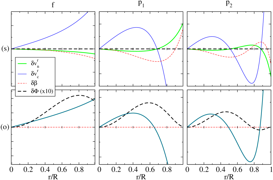
Figure 2: The first three quadrupolar ($l=2$) eigenmode doublets ($\mathrm{o}$)/($\mathrm{s}$) for the background model I. In the case of the $\mathrm{o}$ – modes, the two fluids are comoving to numerical precision, therefore the $\delta v_{\rm n}$ and $\delta v_{\rm c}$ curves can not be seen separately.

Let us first consider the special separable case of the non–stratified model I. The first three pairs of eigenfunctions are presented in Fig. 2, and we see that in the “$\mathrm{o}$” modes the two fluids are comoving, resulting in a non–zero $\delta\Phi$, and they also remain in strict chemical equilibrium, i.e. $\delta\beta=0$. These “ordinary” modes are actually identical to the normal–fluid modes of the same background (see Sect. 5.4). In the case of the $\mathrm{s}$–type modes the two fluids are counter–moving in exactly such a way that the total density remains constant, i.e. $\delta\rho=0$ and therefore $\delta\Phi=0$, while the fluids are driven out of chemical equilibrium, i.e. $\delta\beta\not=0$. The number of radial nodes in $\delta\@vec{v}^{r}$ is the same for the $\mathrm{o}$ and $\mathrm{s}$ modes, and corresponds exactly to their index. All these results confirm the analytic predictions for non–stratified models in Sect. 4.3.

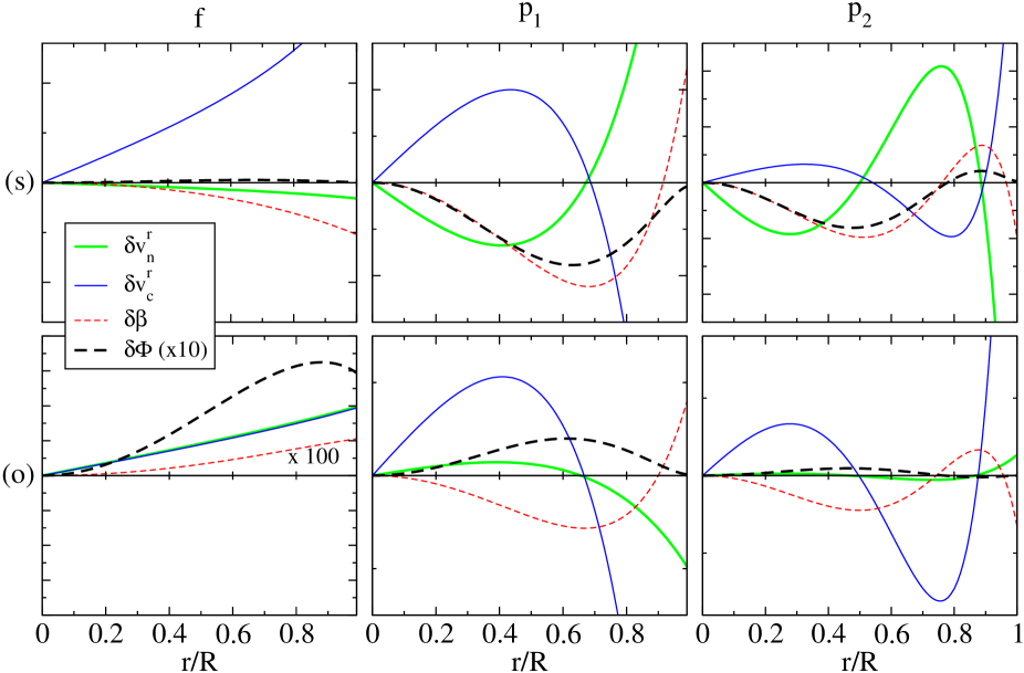
Figure 3: The first three quadrupolar ($l=2$) eigenmode doublets ($\mathrm{o}$)/($\mathrm{s}$) for the background model II. The value of $\delta\beta$ in the lower left figure has been multiplied by 100, in order to show that it is non–zero.

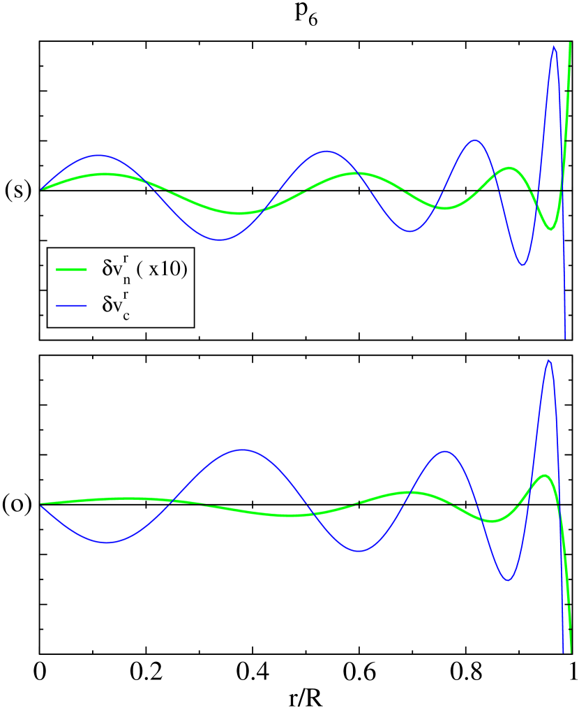
Figure 4: The p₆ eigenmode doublet ($\mathrm{o}$)/($\mathrm{s}$) (for $l=2$) for the background model II. The radial velocity $\delta v^{r}_{\rm n}$ has been multiplied by 10 for better visibility. Neither mode is co– or counter-moving, and the number of radial nodes differs between the two fluids.

However, it would be wrong to assume that these properties are generally true for superfluid oscillations. Stratification makes this picture more complex, even in the case of locally uncoupled fluids considered in this section. If we look at the first three pairs of eigenfunctions for the model II in Fig. 3, we see that the “$\mathrm{o}$” modes are not comoving at all (only the f^o is nearly comoving), and they have non–zero $\delta\beta$, while the “$\mathrm{s}$” modes have non–zero $\delta\rho$ and $\delta\Phi$. One can not say either that the relative amplitude of $\delta\beta$ would be different between the $\mathrm{o}$– and $\mathrm{s}$– cases, as Lindblom & Mendell (1994) wrongly induced from the properties of the f^o–mode, the only eigenmode they presented.

In the case of the low–order modes presented in Fig. 2, the number of radial nodes still seems to correspond to the index, and the fluids are roughly in opposite phase in the $\mathrm{s}$– modes, while they are approximately in phase for the $\mathrm{o}$–modes. Even this, however, is not true in general, as can be seen in Fig. 4 which shows the higher order p₆–modes. In this case neither $\mathrm{o}$– nor $\mathrm{s}$– are dominantly in phase or in opposite phase, and the two radial velocities have different numbers of radial nodes. Therefore neither the index nor the $\mathrm{o}$/$\mathrm{s}$ label bear any reliable information about the properties of the modes. This behaviour is possible because the that this eigenvalue problem is not of Sturm–Liouville type except in the non–stratified case.

$l=0$	$\omega_{I}$	$\omega_{II}$	$\omega_{III}$
fo	0.616 801 012	0.860 501 159	0.539 820 916
fs	0.825 395 141	1.004 218 360	0.713 202 951
p${}_{1}^{\mathrm{o}}$	1.272 153 763	1.650 440 676	1.114 032 342
p${}_{1}^{\mathrm{s}}$	1.398 557 067	1.780 808 966	1.186 350 906
p${}_{2}^{\mathrm{o}}$	1.855 852 617	2.326 264 710	1.582 750 279
p${}_{2}^{\mathrm{s}}$	1.949 822 942	2.573 698 536	1.675 075 045
p${}_{3}^{\mathrm{o}}$	2.418 457 671	2.985 429 110	2.018 290 454
p${}_{3}^{\mathrm{s}}$	2.493 326 179	3.352 297 316	2.169 556 932
p${}_{4}^{\mathrm{o}}$	2.970 977 248	3.638 960 946	2.445 611 455
p${}_{4}^{\mathrm{s}}$	3.033 169 591	4.122 179 788	2.658 934 809

Table 3: Frequency spectrum of radial eigenmodes ($l=0$) for models I, II and III in natural units $\omega_{0}=\sqrt{4\pi G\rho_{0}}$.

$l=1$	$\omega_{I}$	$\omega_{II}$	$\omega_{III}$
fo	$0^{a}$	$0^{a}$	$0^{a}$
fs	0.389 835 134	0.440 176 989	0.387 577 390
p${}_{1}^{\mathrm{o}}$	0.898 011 966	1.191 707 859	0.798 353 611
p${}_{1}^{\mathrm{s}}$	1.040 570 747	1.280 907 920	0.895 985 737
p${}_{2}^{\mathrm{o}}$	1.518 621 841	1.930 140 941	1.317 638 486
p${}_{2}^{\mathrm{s}}$	1.621 023 028	2.105 369 668	1.384 086 979
p${}_{3}^{\mathrm{o}}$	2.099 218 641	2.609 579 518	1.770 672 472
p${}_{3}^{\mathrm{s}}$	2.179 811 073	2.908 118 483	1.887 282 252
p${}_{4}^{\mathrm{o}}$	2.662 623 840	3.274 392 031	2.206 080 421
p${}_{4}^{\mathrm{s}}$	2.729 000 908	3.692 629 614	2.385 023 708

Table 4: Frequency spectrum of dipolar eigenmodes ($l=1$) for models I, II and III in natural units $\omega_{0}=\sqrt{4\pi G\rho_{0}}$. ^a The zero frequency modes correspond to the analytic result of a constant displacement field $\@vec{\xi}$. This solution can not be produced by our code because the equations have been expressed in terms of velocities instead of displacements.

$l=2$	$\omega_{I}$	$\omega_{II}$	$\omega_{III}$
fo	0.390 550 961	0.424 294 338	0.376 662 787
fs	0.526 990 499	0.604 904 572	0.516 636 947
p${}_{1}^{\mathrm{o}}$	1.101 827 434	1.423 800 575	0.980 798 266
p${}_{1}^{\mathrm{s}}$	1.206 881 695	1.514 568 856	1.039 415 772
p${}_{2}^{\mathrm{o}}$	1.723 444 868	2.164 156 378	1.478 705 720
p${}_{2}^{\mathrm{s}}$	1.806 873 473	2.380 237 199	1.557 015 636
p${}_{3}^{\mathrm{o}}$	2.310 315 782	2.858 007 106	1.932 213 886
p${}_{3}^{\mathrm{s}}$	2.379 342 400	3.200 741 221	2.072 313 682
p${}_{4}^{\mathrm{o}}$	2.879 785 468	3.533 905 837	2.372 551 143
p${}_{4}^{\mathrm{s}}$	2.938 448 588	3.997 594 591	2.576 350 147

Table 5: Frequency spectrum of quadrupolar eigenmodes ($l=2$) for models I, II and III in natural units $\omega_{0}=\sqrt{4\pi G\rho_{0}}$.

An interesting fact to notice in tables 3 to 5 is that the fundamental modes (f^o and f^s) are the lowest frequency modes in the spectrum, in other words there are no g–modes present (which usually lie far below the f–mode) in these superfluid models. This confirms the numerical findings by Lee (1995) and the local analysis of Andersson & Comer (2001a).

The absence of g-modes can be made clearer when acoustic modes and surface gravity modes are filtered out. The latter modes are easily removed by suppressing surface motions and imposing therefore $W_{X}=0$ at the star surface. Acoustic modes, on the other hand, are filtered out by using the so-called anelastic approximation which makes an expansion in powers of the Brunt-Väisälä frequency (see Dintrans & Rieutord 2001; Rieutord & Dintrans 2002). Using this approximation mass conservation now reads

$$\@vec{\nabla}\cdot(\rho_{n}\delta\@vec{v}_{\rm n})=0\quad{\rm and}\quad\@vec{\nabla}\cdot(\rho_{c}\delta\@vec{v}_{\rm c})=0$$ (94)

instead of (45) and (46). In the case we have considered, i.e. that of no entrainment ($\alpha=0$), the equations of motions read:

$$\@vec{\nabla}(\delta\widetilde{\mu}^{\rm n}+\delta\Phi) = -i\omega\delta\@vec{v}_{\rm n}\,,$$ (95)

$$\@vec{\nabla}(\delta\widetilde{\mu}^{\rm c}+\delta\Phi) = -i\omega\delta\@vec{v}_{\rm c}\,,$$ (96)

$$\nabla^{2}\delta\Phi = k_{\rm n}\,\delta\widetilde{\mu}^{\rm n}+k_{\rm c}\,\delta\widetilde{\mu}^{\rm c}\,,$$ (97)

Using (94), we eliminate the velocities and are left with the system:

$$\@vec{\nabla}\cdot\left(\rho_{n}\@vec{\nabla}(\delta\widetilde{\mu}^{\rm n}+\delta\Phi)\right) = 0\,,$$ (98)

$$\@vec{\nabla}\cdot\left(\rho_{c}\@vec{\nabla}(\delta\widetilde{\mu}^{\rm c}+\delta\Phi)\right) = 0\,,$$ (99)

$$\nabla^{2}\delta\Phi = k_{\rm n}\,\delta\widetilde{\mu}^{\rm n}+k_{\rm c}\,\delta\widetilde{\mu}^{\rm c}\,,$$ (100)

where we see that the mode frequency has disappeared. Using the boundary conditions, it turns out that the only solution is $\delta\widetilde{\mu}^{\rm c}=\delta\widetilde{\mu}^{\rm n}=\delta\Phi=0$, thus showing that no eigenmode exists when acoustic and surface gravity modes are filtered out.

However, the presence of g–modes due to chemical composition gradients in normal–fluid neutron star models has been pointed out by Reisenegger & Goldreich (1992), and their possibly observable excitation in a coalescing binary neutron star has been discussed by Reisenegger & Goldreich (1994) and Lai (1994). We will see in Sect. 5.4 that these predicted composition g–modes do indeed appear in the normal–fluid case. In principle the presence or absence of these modes could therefore be used as a possibly observable indicator for superfluidity in neutron stars.

5.3.2 The effect of coupling by entrainment

In this section we study the dependence of the mode-frequencies and properties on the coupling by entrainment. Obviously, we only need to specify one entrainment function, $\varepsilon_{\rm c}$ say, as $\varepsilon_{\rm n}$ is then determined by (6). Because the uncertainties and differences of the “realistic” models for $\varepsilon_{\rm c}$ provided by nuclear physics calculations so far are still considerable, we chose the simplest entrainment model, namely $\varepsilon_{\rm c}=\varepsilon$ being a constant. The value of this constant $\varepsilon$ can be related to the proton effective mass $m_{\rm p}^{*}$ (22), and is roughly constrained from the nuclear physics calculations (Chao et al. 1972; Sjöberg 1976; Baldo et al. 1992; Borumand et al. 1996) to lie in the range $0.3\leq\varepsilon\leq 0.7$. We nevertheless consider the broader range between $-0.8\leq\varepsilon\leq 0.8$ to demonstrate the qualitative behaviour more clearly. This will also show that the “locally uncoupled” case $\varepsilon=0$ (considered in the previous section) is not special, contrary to what one might have expected.

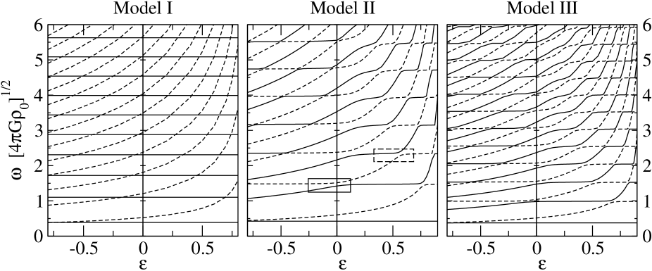
Figure 5: Eigenmode frequencies $\omega$ (for $l=2$) as functions of entrainment $\varepsilon$ for models I, II and III. The full and dashed lines represent the frequencies of the modes denoted respectively by $\mathrm{o}$ and $\mathrm{s}$ in table 5. The avoided crossings marked by the full and the dashed box are represented in terms of the eigenfunctions in Figs. 6 and 7. We note that for models II and III all crossings shown are avoided.

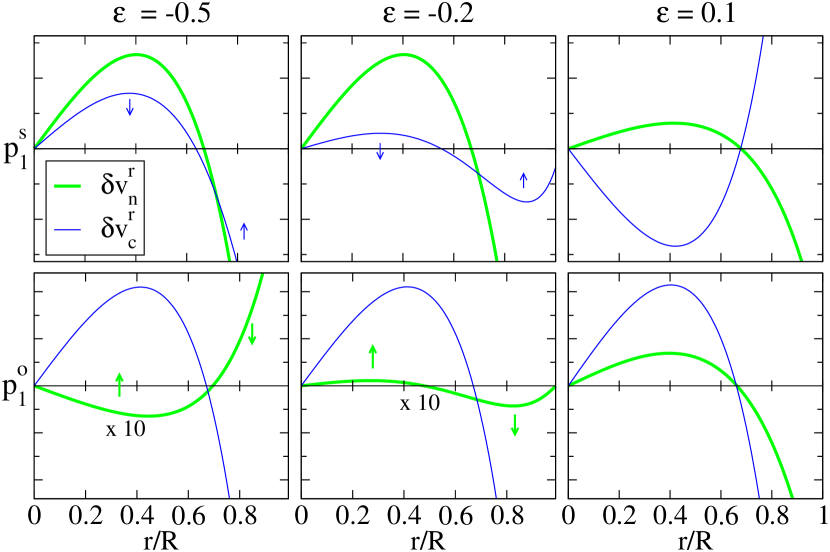
Figure 6: Avoided crossing between the p${}_{1}^{\mathrm{o}}$ and the p${}_{1}^{\mathrm{s}}$ modes of Model II (for $l=2$), indicated by the box in Fig. 5. The three columns show the corresponding eigenfunctions for three different values of entrainment. The small arrows indicate the “evolution” of the eigenmode when increasing $\varepsilon$. The $\delta v_{\rm n}^{r}$ curves in the two lower left figures have been magnified by a factor of $10$.

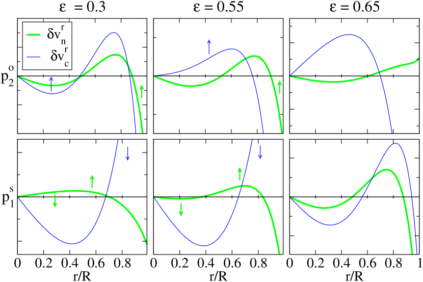
Figure 7: Avoided crossing between the p${}_{1}^{\mathrm{s}}$ and the p${}_{2}^{\mathrm{o}}$ modes of Model II ($l=2$), indicated by the hatched box in Fig. 5. The three columns show the corresponding eigenfunctions for three different values of entrainment. The small arrows indicate the “evolution” of the eigenmode when increasing $\varepsilon$.

The results for the mode-frequencies as functions of $\varepsilon$ for the three background models are represented in Fig. 5. In the case of the non–stratified model I, we observe the predicted (sect. 4.3) decoupling, and in particular the independence of the “ordinary”–type modes of entrainment. Because of this decoupling the respective frequencies of the two mode families can simply cross each other when $\varepsilon$ is varied. In the generic stratified models (model II and III), the modes of the doublets are coupled and avoided crossings result when mode–frequencies come to close to each other, as also found recently by Andersson et al. (2002). In this process of avoided crossing the two modes seem to exchange some of their respective properties of being dominantly “co-” or “counter-moving”, as can be seen in Fig. 6), and they also can exchange their number of radial nodes, as we see in the avoided crossing of the p${}_{1}^{\mathrm{s}}$ and p${}_{2}^{\mathrm{o}}$ in Fig. 7.

Another important conclusion can be drawn from Fig. 5, namely that the “locally uncoupled” case $\varepsilon=0$ discussed in the previous section does not represent a special case in any respect, because the two fluids are always coupled through $\delta\Phi$. The effect of $\varepsilon$ is simply to change the coupling, but no configuration is completely uncoupled. On can see in Fig. 5 that several avoided crossings happen practically at $\varepsilon=0$, which is the case in particular for the p₆-modes of model II presented in Fig. 4.

5.4 The one–fluid case: recovering the g–modes

Following the discussion in sect. 3.2, the one–fluid case is defined by $\delta\@vec{v}_{\rm n}=\delta\@vec{v}_{\rm c}\equiv\delta\@vec{v}$. We only have one Euler equation in this case, which in the harmonic decomposition (54) has the two components

$$x_{\rm n}\,{\delta\widetilde{\mu}^{\rm n}}^{\prime}+x_{\rm c}\,{\delta\widetilde{\mu}^{\rm c}}^{\prime}+\delta\Phi^{\prime} = -{i\omega\over r}\,W\,,$$ (101)

$$x_{\rm n}\,\delta\widetilde{\mu}^{\rm n}\,+x_{\rm c}\,\delta\widetilde{\mu}^{\rm c}\,+\delta\Phi\, = -i\omega\,V\,.$$ (102)

These two equations replace (57)–(60), while the remaining equations of this system are unchanged (subject to the substitutions $W_{\rm n}=W_{\rm c}=W$ and $V_{\rm n}=V_{\rm c}=V$). The eigen-frequencies of this system are shown in table 6, where we see the presence of composition g–modes as expected for all models with stratification. This is consistent with the prediction by Reisenegger & Goldreich (1992) and the numerical findings of Lee (1995).

$l=2$	$\omega_{I}$	$\omega_{II}$	$\omega_{III}$
…	–	…	…
g4	–	0.012 105 268	0.011 489 709
g3	–	0.015 003 335	0.014 157 505
g2	–	0.019 814 997	0.018 492 575
g1	–	0.029 631 110	0.026 880 058
$f$	0.390 550 961	0.424 310 492	0.376 717 911
p1	1.101 827 434	1.477 988 230	0.988 324 062
p2	1.723 444 868	2.348 478 094	1.533 337 250
p3	2.310 315 782	3.163 853 143	2.050 348 013
p4	2.879 785 468	3.954 289 860	2.552 745 872
…	…	…	…

Table 6: The eigenvalue spectrum (for $l=2$) for the models I,II, and III. The non–stratified model I has no g–modes.

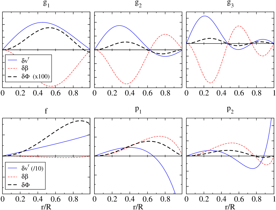
Figure 8: The first few ($l=2$) g–, f– and p–modes for model II. We note that the g–modes are characterised by a very small radial velocity $\delta v^{r}$ at the surface, while it is very large in the case of p–modes.

We also see that in the non–stratified model I, the one–fluid frequencies and modes correspond exactly to the corresponding “ordinary”-type solutions of the two–fluid case (see table 5 and Fig. 2), as would be expected from the separability of the system as discussed in Sect. 4.3.

We note that the perfect fluid modes of stratified models generally have $\delta\beta\not=0$, because adiabatic oscillations generally drive fluid elements out of equilibrium, only in the non–stratified case (model I) is $\delta\beta=0$ strictly satisfied.

The absence/presence of $g$–modes in superfluid/normal fluid models might seem somewhat surprising but one can get a better intuitive understanding by considering the physical origin of these $g$–modes: a radially displaced fluid element will remain close to mechanical (pressure) equilibrium with its surroundings, but its respective values of $\rho_{\rm n}$ and $\rho_{\rm c}$ will generally differ from the surroundings (i.e. when $x_{\rm c}^{\prime}\not=0$) and therefore (via the equation of state) its total density will also be different, resulting in a buoyant restoring force and a corresponding oscillation mode (in unstable models this restoring force will actually drive the fluid element still further away from its initial position, leading to convection). In the simple (cold) superfluid models considered here, each fluid element of either fluid (${\rm n}$ or ${\rm c}$) is only characterised by a single quantity, namely $\rho_{\rm n}$ or $\rho_{\rm c}$. Displacing an element of fluid ${\rm n}$, say, will therefore result not only in mechanical equilibrium ($\widetilde{\mu}^{\rm n}$), but also in buoyant equilibrium. This can by seen by expressing its density at the new position as $\rho_{\rm n}=\rho_{\rm n}(\widetilde{\mu}^{\rm n},\rho_{\rm c})$. The fluid ${\rm c}$ was not displaced, therefore not only $\widetilde{\mu}^{\rm n}$ but also $\rho_{\rm c}$ of the fluid element are identical to the background values, and so is $\rho_{\rm n}$. If we had allowed for an additional comoving quantity like entropy $s$, we would expect to find g–modes driven by a stratification in $s/\rho_{\rm n}$.

It is intriguing to see that the absence of the $g$–modes in superfluid models is accompanied by an apparent doubling of acoustic modes, but it is not obvious to establish a link between these different classes of modes as we are currently not aware of a continuous transition from a two–fluid to a one–fluid model (either the two fluids are locked together or they are not).

6 Conclusions

In this paper we have tried to clarify the qualitative properties of the eigenmode spectrum of superfluid neutron stars, using a simple two–fluid model. We have shown the important — previously somewhat overlooked — role of stratification for these modes. The picture has been found to be more complex than previous studies have suggested, and some of the earlier conclusions have been shown to apply only for non–stratified models. In particular, one can not generally talk about two distinct families of “superfluid” and “ordinary” modes. The system of equations describing two–fluid modes can not be separated in the case of stratified stars, and its solutions have no direct correspondence to the eigenmodes of the one–fluid system. The two–fluid modes are generally neither co– nor counter-moving, rather all of them are characterised by non–zero amplitudes of relative velocity $\delta\@vec{\Delta}$, deviation of chemical equilibrium $\delta\beta$ and total density perturbation $\delta\rho$. Also the order of the mode does not necessarily correspond to the number of radial nodes (as seen in Fig. 4), which is possible because the system is not of the Sturm–Liouville type. We have further confirmed earlier findings about the absence of g–modes in these superfluid models (Lee 1995; Andersson & Comer 2001a), as well as the appearance of avoided crossings between mode frequencies when changing the entrainment parameter (Andersson et al. 2002).

Given the radical difference and richer structure of the oscillations of superfluid neutron star models as compared to the simple perfect fluid models, we think that much future effort is needed to further clarify these properties and evaluate possibly observable consequences. The respective absence and presence of g–modes in these two different models is a striking example of such a potentially observable indicator of superfluidity in neutron stars. However, many more physical effects have to be taken into account in order to achieve a more realistic description of superfluid neutron stars, namely the inclusion of vortex–forces and beta reactions, both of which will lead to dissipation. Furthermore, an “envelope” or an elastic crust should be included, and maybe most importantly, the effects of rotation and magnetic field, which add new restoring forces and result in a much richer spectrum of modes. Eventually, for a realistic study of oscillations of superfluid neutrons stars, one needs to work in a generally relativistic framework, as pioneered by Comer et al. (1999) and Andersson et al. (2002). This step is crucially important also for the assessment of the gravitational radiation emitted by these modes, and their stability/instability via the CFS mechanism (Friedman & Schutz 1978).