A Computer Program to visualize Gravitational Lenses

Abstract

Gravitational lenses are presently playing an important role in astrophysics. By means of these lenses the parameters of the deflector such as its mass, ellipticity, etc. and Hubble’s constant can be determined. Using C, Xforms, Mesa and Imlib a computer program to visualize this lens effect has been developed. This program has been applied to generate sequences of images of a source object and its corresponding images. It has also been used to visually test different models of gravitational lenses.

1 Introduction

Computer visualization is nowadays an important field of scientific research, because it often allows a better understanding of natural phenomena.

Gravitational lenses (hereafter GL), predicted by Einstein’s general relativity theory, deflect the light rays coming from a distant object. GL’s allow the formation of mutiple images of the same source object. Moreover this gravitational effect opens the possiblity of determining the mass of the deflector and the computation of the age of the Universe (Hubble’s constant), as well as other lens parameters and cosmological parameters.

An interactive computer program to visualize this gravitational effect has been developed. The program was written in the C programming language and uses the Xforms (tool kit), Mesa (graphic library) and Imlib (image library). The program runs on systems with Linux or Unix. An SGI version of this program is also available.

In the first section the gravitational lens effect is briefly reviewed. The visualization program is presented in the second section. In the third section some applications are shown: image sequences and easy visual modelling. Improved versions of this program can be produced and the author wishes to invite the interested reader to participate in this process. The author is preparing a website for downloading this program:

http://cinespa.ucr.ac.cr/software/xfgl/index.html

2 The Gravitational Lens Theory

2.1 The Gravitational Lens Equation

Due to the curvature of space-time, light rays coming from a distant source object (quasar, star or galaxy) are deflected when passing close to a lens or deflector (star, galaxy or cluster of galaxies). For weak gravitational fields the Post-Newtonian approximation is applicable. Under this approximation the deflection angle or Einstein’s angle does not depend on the direction of propagation and the trayectory are approximated by straight lines. This gravitational light deflection is depicted in figure 1. From this figure an equation, the GL equation or the ray tracing equation which is obeyed by light rays passing near a lens object can be deduced:

$${\bf y}={\bf x}-{{\mbox{\boldmath$\alpha$}}}{(\bf x)}\;\;,$$ (1)

where

$${{\mbox{\boldmath$\alpha$}}}({\bf x})={{1}\over{\pi}}\int\!\kappa({\bf x}^{\prime}){{({\bf x}-{\bf x}^{\prime})}\over{|{\bf x}-{\bf x}^{\prime}|^{2}}}d^{2}{\bf x}^{\prime}\;\;,$$ (2)

$${\bf y}={{\mbox{\boldmath$\eta$}}\over{\eta_{0}}}={{D_{s}{\mbox{\boldmath$\beta$}}}\over{\eta_{0}}}\qquad,\qquad{\bf x}={{\mbox{\boldmath$\xi$}}\over{\xi_{0}}}={{D_{l}{\mbox{\boldmath$\theta$}}}\over{\xi_{0}}}\qquad,\qquad\eta_{0}={{D_{s}}\over{D_{l}}}\xi_{0}$$ (3)

and $\xi_{0}$ is the length scale on the lens surface. The angle ${{\mbox{\boldmath$\alpha$}}}({\bf x})$ is called the Einstein’s angle. The surface density of the lens is given by

$$\kappa({\bf x})={{\Sigma({\mbox{\boldmath$\xi$}})}\over{{\Sigma}_{cr}}}\;\;,$$ (4)

where $\Sigma_{cr}$ represents the critical density:

$$\Sigma_{cr}={{c^{2}D_{s}}\over{4\pi D_{l}D_{ls}}}\;\;.$$ (5)

A generalization of equation (1) which considers the perturbation of a macrolens (a galaxy or cluster of galaxies) is given by

$${\bf y}={\cal M}\cdot{\bf x}-{{\mbox{\boldmath$\alpha$}}}{(\bf x)}\;\;,$$ (6)

where the matrix ${\cal M}$ is given by the expression

$${\cal M}=\left(\begin{array}[]{ccc}1-\kappa-\gamma\cos{\phi}&-\gamma\sin{\phi}\\ -\gamma\sin{\phi}&1-\kappa+\gamma\cos{\phi}\end{array}\right)\;\;.$$

The components of the matrix depend upon the parameters $\kappa$ and $\gamma$ and $\phi$ which are respectively the dimensionless constant surface mass density, the dimensionless shear of the macrolens and the shear angle. The microlens (a star in a galaxy or a galaxy in a cluster of galaxies) is represented by means of the Einstein’s angle ${{\mbox{\boldmath$\alpha$}}}({\bf x})$.

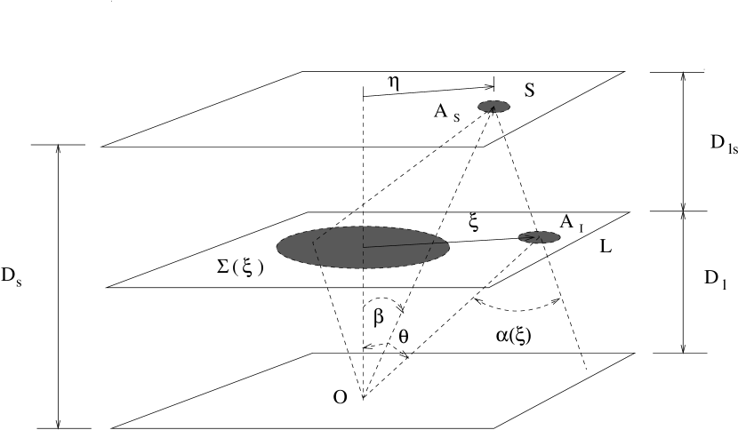
Figure 1: The Post-Newtonian approximation of the light deflection

2.2 Gravitational Lens Models

To simulate Einstein’s angle there are several models for the lens mass distribution. The gravitational lens models are divided as follows:

• Parametric models

• Non-parametric models.

At the present time the program has only parametric models^-. The non-parametric models are lately used to model gravitational lenses^-. For weak lensing the Kaiser-Squires method can be applied to model lenses ^-. In the program these techniques have not been implemented.

The program includes the following parametric models:

• Chang Refsdal Model,

• Double Plane Lens,

• Transparent Sphere,

• Singular Isothermal Sphere,

• Nonsingular Isothermal Sphere,

• Elliptical Model,

• King Model,

• Truncated King Model,

• Hubble Model,

• De Vaucouleur Model,

• Spiral Model,

• Multipole Lens,

• Rotation Lens and

• Uniform Ring.

The interested reader is refered to the literature for a discussion of these models^-.

3 The Visualization program

3.1 Description of the program

The program was written in C and the Mesa graphic libraries (free version of the Open GL) have been used. These graphic subroutines are available for Unix or Linux systems. The XForms Library was used to designed the control panel program (see fig. 2). The Image Library permits to load an image file on the program. These libraries can be found at the following addresses:
http://bragg.phys.uwm.edu/xform
http://www.mesa3d.org/
ftp://ftp.enlightenment.org/pub/enlightenment/imlib/

The program creates a window: the Control Panel (see fig. 2). The user can control all item on it by clicking. A second window, the Image window, appears when the Image Window button is clicked on this panel (see fig. 3). The Help button on the panel give the user a concise program guide.

A version of this program which employs the SGI Graphic Libraries is also available.

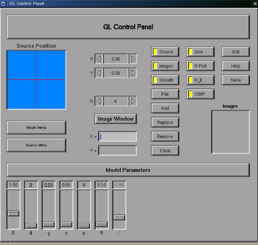
Figure 2: Control Panel

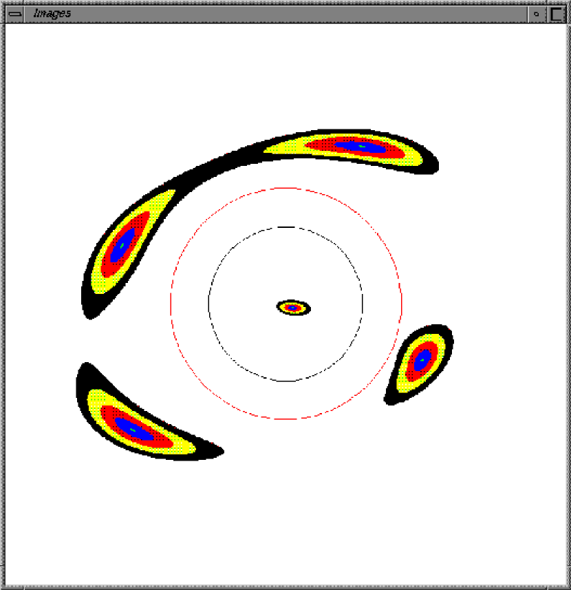
Figure 3: The Image Window

3.2 The Control Panel

All the objects are adjusted interactively with the mouse. This control panel interface has the following items:

• Source Menu (Filled Circle, Coloured Rings and Image File)

• Model Menu (the aforementioned models)

• Source Positioner

• Three counters, two for source positioning (X, Y) and one for adjusting the pixel resolution (N)

• Two inputs for positioning the observed lense images (X, Y)

• Buttons (Model Paramters, Image Window, Source, Images, Smooth, Grid, R Plot, R_E, File, Add, Replace, Remove, Clear, OBIP, Save, Help, Exit),

• Sliders (if one chooses a model, then the corresponding sliders appear)

• A browser for showing the observed lense images

For a detailed discussion of these items see the manual program (to get the program manual send an email to the author or click the Help button on the control panel).

3.3 The Image Window

On this window the events (images, ray plot, etc.) appear. All variations of the parameters on the control panel are shown immediately on this window. To show the images of a chosen gravitational lens model the ray tracing method has been used. The caustic is represented by means of the ray plot method.

4 Applications

In this section two of many applications of the program are discussed:

• Image sequences

• Easy visual modeling

An image sequence for an elliptical model and a visual modeling of the gravitational lens $2237+0305$ will be shown.

4.1 Image sequences

An image sequence is easy to generate with this program. The structure of the images for different positions of the source can be investigated by means of such an image sequence.

An Elliptical Lens

A sequence of images is shown in figure 4. The sequence begins on the top left-hand-side panel of the sequence. The source, concentric rings, moves from left to right. The source is not shown, only the images. The best possible resolution given by the control panel was used. In this sequence the shear $\gamma$ and the constant surface mass density $\sigma$ are non zero and the shear angle $\phi=0$. There are two circles: the Einstein ring or lens scale and the core radius. The formation of a small and a large arc can be seen. In the middle of the sequence one can recognize the deformation of the Einstein ring in an ellipse. Due to the core radius an image appears in the centre, which fuses with an arc, in the case that the source moves away.

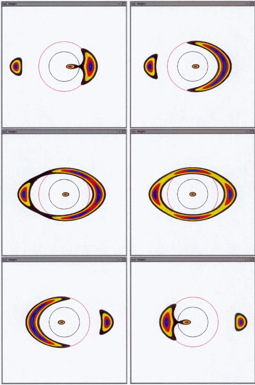
Figure 4: An elliptical lens

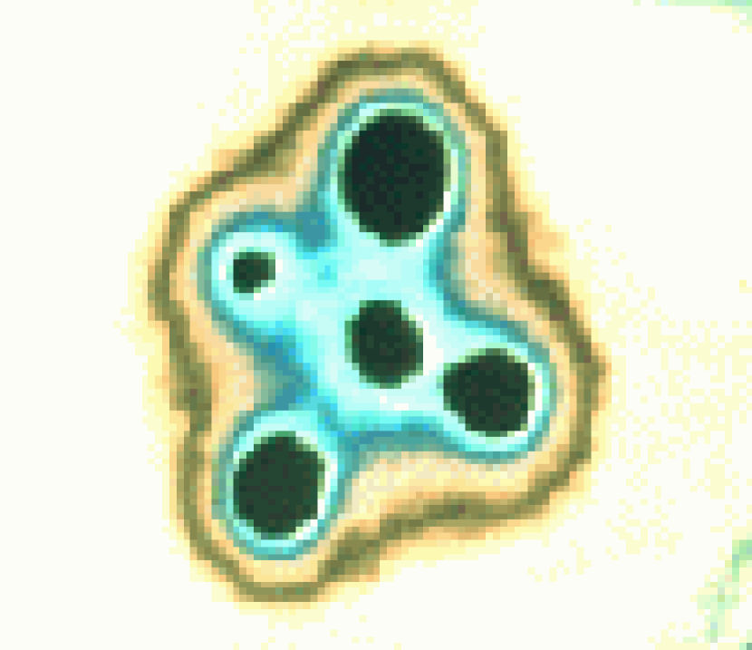
Figure 5: Gravitational lens $2237+0305$

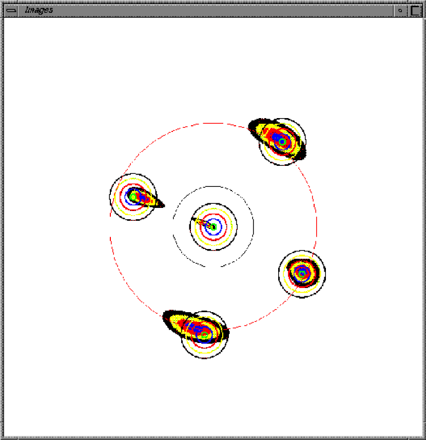
Figure 6: Visual fitting of the gravitational lens $2237+0305$

4.2 Easy Visual Modeling

Here an easy visual modeling of the gravitational lens system $2237+0305$ is shown. The model images are considered well-fit when they overlap most of the area of the observed images (represented through concentric circles), as visually estimated. At the present time a fitting subroutine is not implemented. When such a subroutine is included, this program would become an excellent tool to model gravitational lenses.

Visual Model for the Gravitational Lens $2237+0305$

The system $2237+0305$ [see fig. 5] was discovered in 1985. Due to its unusual shape this lens is called Einstein cross. Attempts to model this lens have been carried out^-

The data used in tables 1 and 2, was taken from Kent and Falco, and Schneider et al.^- The cosmological distances of table 2 were calculated using the equations from Schneider et al. ($H_{0}=100\,{\rm km}\,{\rm s}^{-1}\,{\rm Mpc}^{-1}$ and $q_{0}=1/2$).

Table 1: Image positions for the lens $2237+0305$

	Positions
Object	X	Y
	$(^{\prime\prime})$	$(^{\prime\prime})$
2237 $+$ 0305 A	$0.08\pm 0.01$	$-0.94\pm 0.01$
2237 $+$ 0305 B	$-0.60\pm 0.02$	$0.74\pm 0.01$
2237 $+$ 0305 C	$0.70\pm 0.01$	$0.26\pm 0.01$
2237 $+$ 0305 D	$-0.77\pm 0.02$	$-0.41\pm 0.02$
Galaxy	$0.00\pm 0.02$	$0.00\pm 0.02$

Table 2: Parameters of the lens galaxy and the source

Parameter	Value
$z_{l}$	$0.0394$
Distance $D_{l}$	$110\,{\rm Mpc}$
Ellipticity $\epsilon$	$0.57$
Angle of the mayor axis	$77^{\circ}$
Angle of the bulk	$38^{\circ}$
Velocity dispersion $\sigma_{v}$	$215\,{\rm km}/{\rm s}$
$z_{s}$	$1.695$
Distance $D_{s}$	$867\,{\rm Mpc}$
Distance $D_{ls}$	$825\,{\rm Mpc}$

Since the positions of the observed images [table 1] are too small to be shown in the image window, a scale factor of $200$ was chosen (the scale factor can be chosen by the user). Then all positions are multiplied by this scale. The positions are also rotated around the $X$ axis.

The lens galaxy is elliptical, so it is reasonable to choose an elliptical model in the program, although one can also try other models^-. A lens model of $N$ ($N=6724$) point masses was used by Schenider et al.. An elliptical King model and an elliptical de Vaucouleur model were used in Kent and Falco. In Rix et al. a the de Vaucouleur model was used. A general SIS model with shear was used in Wambsganss and Paczynski.

The lens major axis has a particular orientation, therefore the coordinate system is rotated around an angle $\theta$, so that the elliptical potential has the same orientation. The angle $\theta$ is taken as a parameter. The constant surface mass density and the shear are zero. The visual fitting is shown in fig. 5. In table 3 the model parameters of the elliptical model are shown. These were found through variation of sliders and source positioners.

Table 3: Model parameter of the elliptical model and source position

Parameter	Value
E: Lens scale	$180$
$\theta$: Rotation angle	$336^{\circ}$
$\gamma$: Shear	$0$
$\sigma$: Constant surface mass density	$0$
$\phi$: Shear angle	$0^{\circ}$
R: Source Radius	$50$
C: Core scale	$70$
$\epsilon$: Ellipticity	$0.54$
$\alpha$: Softness	$0.05$
$\kappa$: Constant Central mass density	$1.00$
(X, Y): Source Position	$(28.0,\,12.0)$

The data for the lens scale (Einstein Radius), the core scale and the source position must be divided by $200$. So one obtained ${\alpha}_{E}=0^{\prime\prime}.90$ , $\theta_{c}=0^{\prime\prime}.35$ and $(X,\,Y)=(0^{\prime\prime}.14,\,0^{\prime\prime}.06)$ . The Einstein radius and core radius are determined by means of the equations ${\cal R}_{E}={\alpha}_{E}D_{l}$ and $r_{c}=\theta_{c}D_{l}$ (${\cal R}_{E}=0.48\,{\rm Kpc}$ and $r_{c}=0.19\,{\rm Kpc}$).

From the following equation the lens mass can be found

$${\cal R}^{2}_{E}=\frac{4GM}{c^{2}}\frac{D_{l}D_{ls}}{D_{s}}\;\;.$$

The velocity dispersion is determined through an equation from Blandford and Kochanek^-.

The major axis angle can be calculated from $\theta^{\prime}=90^{\circ}+\theta$ ($\theta=-24^{\circ}$).

In table 4 all values for the different models are shown: the elliptical King model (model A), the de Vaucouleur model (model B, the source position is referred to the image A), the generalized SIS model (model C) and the elliptical model. The models A, B and C were fitted. Our elliptical model is not reliable, because the program does not possess a fitting subroutine, but one can estimate and compare with other models.

Table 4: Model parameter for the system 2237 $+$ 0305

	Model
Parameter	A	B	C	Elliptical
Einstein Ring	$0^{\prime\prime}.90$	$0^{\prime\prime}.90$	$0^{\prime\prime}.874$	$0^{\prime\prime}.90$
Shear	$-$	$-$	$0.02$	$-$
Angle of the mayor axis ∘	$66.8$	$68$	$66.84$	$66$
Core Radius kpc	$0.10$	$-$	$-$	$0.19$
Ellipticity $\epsilon$	$0.42$	$0.3$	$-$	$0.54$
Softness $\alpha$	$-$	$-$	$-$	$0.05$
Central surface mass density $\kappa$	$-$	$-$	$-$	$1.00$
Velocity dispersion km/s	$170$	$209$	$-$	$109$
Lens Mass $10^{10}{\cal M}_{\odot}$	$1.2$	$1.08$	$1.49$	$1.15$
Source Position
X	$-0^{\prime\prime}.07$	$0^{\prime\prime}.159$	$-$	$0^{\prime\prime}.14$
Y	$-0^{\prime\prime}.02$	$0^{\prime\prime}.877$	$-$	$0^{\prime\prime}.06$

5 Conclusions and Future Work

From both the didactical and scientific point of view a program to visualize the gravitational lenses is useful. This versatile program works quickly and interactively with the mouse.

With this computer program the user has a tool to visualize and to visually model gravitational lenses. The applications of the program, we have showed in this paper, are:

• Sequences of images

• Easy visual modeling

The user can produce sequences of images for a chosen gravitational lens model. Through the variation of model parameters he or she can investigate the structure of the images. The user can also attempt to visually model observed gravitational lenses. The observed position data can be used as input data and the model parameters can be easily varied in order to approximate the observed images. So the user can quickly obtain model parameter estimations. Some observed lenses have already been modeled and the user can compare those results with the output from a chosen model of the control panel.

Future Work

The program can be improved by the inclusion of some additional subroutines:

• Contour subroutine for the isochrones (time delay)

• Light curves subroutine (dependence of brightness with time)

• Subroutine for computing the image magnification

• Subroutine to calculate critical curves and caustics

• Fitting subroutine

• Root finder subroutine

• Subroutine to load images of observed gravitational lenses

• Subroutine with more complex (elliptical) models

• Subroutine for superposition of models in different lens planes

• Subroutine with cosmic string lens models

• Subroutine for non-parametric reconstruction

• Kaiser-Squires Subroutine

The author is working on implementing some of the abovementioned improvements.

Acknowledgments: The author would like to thank M. Magallón for his contribution in developing part of the software discussed in this paper.

References

P. Schneider, J. Ehlers, E.E. Falco, Gravitational Lenses, A&A Library, Springer, Heidelberg, 1992.

J. Huchra, Galatic Structure And Evolution, in R. Meyers, Encyclopedia of Astronomy and Astrophysics, 203-19, Academic Press, Inc., London, 1989.

F. Frutos-Alfaro, Die interaktive Visualisierung von Gravitationslinsen, PHD Thesis, Eberhard-Karls-Universität Tübingen, 1998.

P. Saha, L. L. R. Williams, Non-parametric reconstruction of the galaxy-lens in PG 1115 + 080, astro-ph/9707356, 31 July 1997.

H. M. Abdel Salam, P. Saha, L. L. R. Williams, Non-parametric reconstruction of cluster mass distribution from strong lensing: modelling Abell 370, MNRAS, 294, 734-746, 1998.

H. M. Abdel Salam, P. Saha, L. L. R. Williams, Non-parametric Reconstruction of Abell 2218 from Combine Weak and Strong Lensing, AJ, 116, 4, 1541-1552, 1998.

N. Kaiser, G. Squires, Mapping the Dark Matter with Weak Gravitational Lensing, ApJ, 404, 441-450, 1993.

P. Schneider, C. Seitz, Steps towards nonlinear cluster inversion gravitational distortions I, A&A, 294, 411-431, 1995.

C. Seitz, P. Schneider, Steps towards nonlinear cluster inversion gravitational distortions II, A&A, 297, 287-299, 1995.

C. Seitz, P. Schneider, Steps towards nonlinear cluster inversion gravitational distortions III, A&A, 318, 687-699, 1997.

Silicon Graphics, Graphics Library Programming Guide, Silicon Graphics, Inc., 1991.

M.H. Overmars, Forms Library: A Graphical User Interface Toolkit for Silicon Graphics Workstations, Department of Computer Science, Utrecht University, 1991.

J. Huchra, M. Gorenstein, S. Kent, I. Shapiro, G. Smith, E. Horine, R. Perley, $2237+0305$: A New and Unusual Gravitational Lens, AJ, 90, 691-6, 1985.

H. Yee, High-Resolution Imaging of the Gravitational Lens System Candidate $2237+030$, AJ, 95, 1331-39, 1988.

D. Schneider, E. Turner, J. Gunn, J. Hewitt, M. Schmidt and C. Lawrence, High-Resolution CCD Imaging And Derived Gravitational Lens Models of $2237+0305$, AJ, 95, 6, 1619-28, 1988.

S. Kent, E. Falco, A Model For The Gravitational Lens System $2237+0305$, AJ, 96, 1570-74, 1988.

H. Rix, D. Schneider and J. Bahcall, Hubble Space Telescope Wide Field Camera Imaging of the Gravitational Lens 2237 + 0305, AJ, 104, 959-67, 1992.

J. Wambsganss, B. Paczynski Parameter Degeneracy in Models of the Quadruple Lens System Q $2237+0305$, AJ, 108, 1156-62, 1994.

M. Irwin, Photometric Variations in the Q 2237 + 0305 System: First Detection of a Microlensing Event, A. J., 98, 1989-94, 1989.

K-H. Chae, D.A. Turnshek, V.K. Khersonsky, Realistic Grid of Models for the Gravitationally Lensed Einstein Cross (Q2237+0305) and its Relation to Observational Constraints, Ap. J., 495, 609-616, 1998.

R. Blandford, C. Kochanek, Gravitational Imaging By Isolated Elliptical Potential Wells. I. Cross Sections, ApJ, 321, 658-75, 1987.

C. Kochanek, R. Blandford, Gravitational Imaging By Isolated Elliptical Potential Wells. II. Probability Distributions, ApJ, 321, 676-85, 1987.