New Limits on the Polarized Anisotropy of the
Cosmic Microwave Background at Subdegree Angular Scales

Abstract

We update the limit from the 90 GHz PIQUE ground-based polarimeter on the magnitude of any polarized anisotropy of the cosmic microwave radiation. With a second year of data, we have now limited both Q and U on a ring of $1^{\circ}$ radius. The window functions are broad: for E-mode polarization, the effective $\ell$ is $\left<\ell_{E}\right>=191_{-132}^{+143}$. We find that the E-mode signal can be no greater than $8.4~{}\mu$K (95% CL), assuming no B-mode polarization. Limits on a possible B-mode signal are also presented.

1 INTRODUCTION

The current limits on cosmic microwave background (CMB) polarization restrict the amplitude of its fluctuations to less than $10~{}\mu$K at 95% CL. At large angular scales, Keating et al. (2001) limit the amplitude to $8~{}\mu$K. At subdegree angular scales, the constraint from Hedman et al. (2001, hereafter H01) is $10~{}\mu$K, while at arcminute scales, Subrahmanyan et al. (2000) set a limit of $10~{}\mu$K. Present estimates of the peak polarized fluctuation amplitude are $\sim 6~{}\mu$K at an angular scale of $\sim 0\fdg 2$ ($\ell\!\sim\!950$). These estimates are based on parameters gleaned from CMB temperature anisotropy measurements (e.g. Pryke et al. 2002; Jaffe et al. 2001; Wang, Tegmark, & Zaldarriaga 2001). While CMB polarization has yet to be detected, its characterization will complement CMB temperature anisotropy data and impact our understanding of: gravitational waves from the inflationary epoch (e.g. Turner 1997, Caldwell, Kamionkowski, & Wadley 1999); peculiar velocities at the surface of last scattering (Zaldarriaga & Harari, 1995); the nature of primordial perturbations (e.g. Spergel & Zaldarriaga 1997); primordial magnetic fields (Kosowsky & Loeb, 1996); and cosmological parity violation (Lue, Wang, & Kamionkowski 1999). Here, we report improved limits derived from new data from the 2001 observing season of the Princeton IQU Experiment (PIQUE) at 90 GHz. We combine the new data with data from the first observing season, and also present a reanalysis of those earlier data. These data pass extensive checks for systematic contamination. Future publications will report results from a 40 GHz polarimeter also deployed during the 2001 observing season, and give details of the instrument.

2 INSTRUMENT, OBSERVATIONS AND CALIBRATION

PIQUE has been described previously (H01). The results reported here are from PIQUE’s broadband 90 GHz correlation polarimeter, which underilluminates a 1.2 m off-axis parabola (Wollack et al., 1997), resulting in a beamsize of $0\fdg 235$. The 84-100 GHz bandpass is divided into three subbands called S0, S1, and S2 (H01). Observations are made of a ring of radius $1^{\circ}$ around the NCP; the telescope site is Princeton, NJ.

The polarimeter observed the sky from 2000 January 19 to 2000 April 2 and from 2000 December 19 to 2001 February 28. These two observing seasons yielded 810 hrs and 660 hrs of raw data, respectively.

The scanning strategy is designed to permit null tests for checking sensitivity to systematics. During both observing seasons, the telescope alternated between two azimuth positions at fixed elevation. Data from the two positions are differenced to remove sensitivity to DC offsets. For the first season these azimuth positions were $\pm 0\fdg 93$, and the elevation was $41\fdg 0$. The telescope therefore measured $\mp Q$ (as defined by the IAU) for two regions separated by six hours in right ascension (RA) on the ring of declination $89^{\circ}$. For the second season the azimuth positions were $\pm 1\fdg 31$, with elevation $40\fdg 3$, so the telescope measured $+U$ for two regions separated by twelve hours in RA on the same ring. The azimuth chop period was 13 seconds until 2001 January 23, at which point it was doubled.

The polarimetry channels are calibrated to 10% using a nutating aluminum flat (H01, Staggs et al. 2002). Constant elevation scans of Jupiter are used to determine pointing accuracy and map the beams. For the second observing season the measured beam FWHM are $0\fdg 235(7)$ in co-elevation and $0\fdg 233(7)$ in elevation, in agreement with measurements from the first season. The absolute pointing offsets in elevation are smaller than $0\fdg 03$. However, early in the second observing season, the encoder suffered a misalignment so that the azimuth offset increased from $+0\fdg 03$ to $+0\fdg 08$. (No concomitant change in beamshape was observed.) Note that we are able to neglect this in the analysis because the overlap between the ideal and misaligned beams is still 85%. In fact, simulations indicate the misalignment has less than a $2\%$ effect on our derived limit.

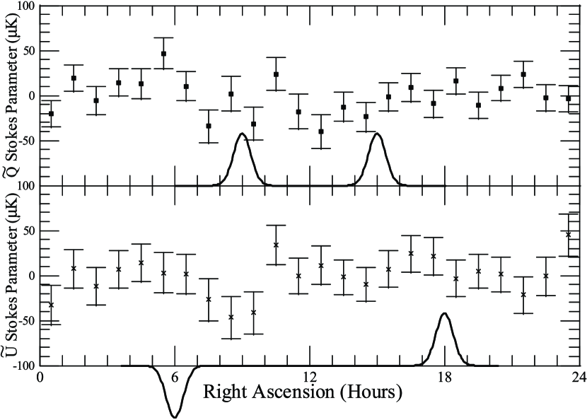
Figure 1: Binned data are shown in thermodynamic units for each observation season. The three frequency channels have been coadded and the one sigma errors include small correlations among the channels. For clarity only 24 approximately beam-sized bins are shown: the actual analysis uses 144 independent bins. Due to PIQUE’s differencing strategies, a 1 Jy point source with 20% polarization located at $\alpha=12^{h}$, $\delta=89^{\circ}$ generates the point source responses shown in the two panels. No such point source is known, and Toffolatti et al. (1998) estimate there are fewer than 200 point sources brighter than 1 Jy in the entire sky at 90 GHz.

3 DATA REDUCTION

The 1470 hours of data from the two observing seasons include: 383 hours of data taken while the telescope was slewing between the desired scan positions, 339 hours of data corrupted by known electromechanical failures, and 59 hours of data in isolated fragments less than 12 hours in length. The remaining 685 hours of data contain 186 hours of data corrupted by meteorological phenomena (clouds), which are identified using the selection criteria described below.

As discussed in H01, the correlation polarimeter suffers a small sensitivity ($\lesssim 0.5$%) to total power because signals reflected from the input of the amplifier in one arm can couple into the other arm through the orthomode transducer. Therefore, the distributions of correlation coefficients

$${\cal C}_{N}=\frac{<S_{i}S_{j}>}{<S_{i}^{2}><S_{j}^{2}>}$$ (1)

between pairs of polarimetry channels $(i,j)$ display large positive tails due to periods of rapid atmospheric fluctuations. Data corrupted by clouds are removed by requiring the coefficients to be less than certain thresholds. Such selection criteria are determined based upon a data set designed to be insensitive to real astronomical polarized signals: the quadrature data (for which data from each scan position are split into halves and differenced). The ${\cal C}_{N}$ are generated as averages over $N$ chops; varying $N$ varies the time scale probed. For purely Gaussian noise, the shapes of the resulting distributions of ${\cal C}_{N}$ for the whole data set depend only on $N$. In order to avoid using additional cutting measures (such as the 6-hr null test used in H01), the ${\cal C}_{N}$-selection technique has been refined from that used for H01. Here, two time scales are used rather than one. First we calculate the average correlation coefficients for segments of the time series 40-70 minutes long (specifically, $N=200$). Segments with coefficients larger than a threshold of 0.20 are removed. Next, coefficients are calculated for $N=50$, for which the cut threshold is 0.32. These thresholds are at $2.5\sigma$ and $2\sigma$, and are chosen so that either cut alone removes $\sim 20$% of the data. The combined cuts remove $27$% of the data. Null test results are not sensitive to the exact values for the thresholds.

The 307(192) hours of data surviving the cuts detailed above from the first(second) observing season are parsed into 144 bins based on the Local Sidereal Time (LST) when the data were taken, following the same procedures outlined in H01. These data are plotted in Figure 1. Offsets on the order of a few hundred $\mu$K are removed from each polarimetry channel for each “deployment” (a period of $>12$ hours bracketed by periods when the instrument was tarped). The results are not sensitive to the exact number of offsets removed. Table 1 presents the results of the null tests described in H01, using the new selection criteria. The $\chi^{2}$ distribution of these null tests is consistent with noise, demonstrating that the data do not suffer from residual atmospheric contamination.

Table 1: Results of $\chi^{2}$ consistency tests.

Year	Test	0000S0	0000S1	0000S2
	Quad	0.96	0.25	0.19
	H1-H2	0.18	0.14	0.33
2000	Pattern	0.46	0.26	0.14
	Si-Sj	0.62	0.83	0.83
	Quad	0.38	0.61	0.28
	H1-H2	0.17	0.61	0.58
2001	Pattern	0.80	0.12	0.38
	Si-Sj	0.47	0.66	0.04

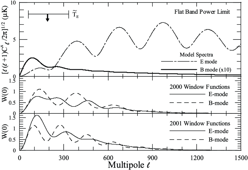
Figure 2: Zero-lag window functions for E- and B-modes (solid and dashed lines) are shown in the middle panel for the 2000 observation season and in the lower panel for the 2001 season. The top panel shows the limit on $T_{E}$ assuming $T_{B}\equiv 0$ for the combined W-band observations. For comparison we also plot (dashed line) E-mode predictions from the best-fit model in Pryke et al. (2002), as well as B-mode predictions (shown in the top panel multiplied by ten) assuming the same model with $T/S=1$.

4 DATA ANALYSIS

The likelihood of a model given a data vector ${\bf x}$ is ${\cal L}\propto\exp(-{\bf{x}}^{T}{\bf{C}}^{-1}{\bf{x}}/2)/|{\bf{C}}|^{1/2}$, where the covariance matrix ${\bf C}$ sums both theoretical correlations from the model (signal) and correlations specific to the experiment (noise): ${\bf C}={\bf S}+{\bf N}$. The analysis of the combined 2000-2001 data uses ${\bf x}$ with 864 elements comprising 144 spatial pixels measured in three different frequency bands over the course of two observing seasons. The noise matrix ${\bf N}$ encodes the variances for each pixel for each channel and also accounts for interchannel correlations from both atmospheric fluctuations weakly coupled into the polarimeter channels and correlated gain fluctuations in the cryogenic amplifiers. The interchannel correlation coefficients are $\leq 8$% on average, and smaller for the two most sensitive channels. (S2 has just $20$% of the total weight.) The noise matrix does not include pixel-pixel correlations, since no such correlations are observed in the time series data. An independent analysis using a 288-element data vector, for which data from the three frequency channels are combined for each spatial pixel, with errors calculated to account for the interchannel correlations, yields consistent results.

Table 2: $95\%$ Confidence Limits

Year	Data	$\widetilde{T}_{E}$	string$\widehat{T}_{E}$	string$\widehat{T}_{B}$
		$(\mu$K)	string$(\mu$K)	string$(\mu$K)
	CMB	12.7	15.8	14.7
	Quad	10.3	13.9	12.9
2000	(H1-H2)/2	14.9	19.7	17.4
	CMB	10.4	15.9	17.8
	Quad	10.4	16.2	18.0
2001	(H1-H2)/2	11.2	17.2	19.4
2000	CMB	8.4	11.2	11.5
$+$	Quad	6.1	8.3	8.4
2001	(H1-H2)/2	8.5	11.5	11.6

Since PIQUE measured $Q$ in 2000 and $U$ in 2001, the signal covariance matrix takes the form:

$${\bf{S}}=\pmatrix{\langle\tilde{Q}\tilde{Q}\rangle&\langle\tilde{Q}\tilde{U}\rangle\cr\langle\tilde{Q}\tilde{U}\rangle&\langle\tilde{U}\tilde{U}\rangle}$$ (2)

where $\langle\tilde{Q}_{i}\tilde{Q}_{j}\rangle$ (or $\langle\tilde{U}_{i}\tilde{U}_{j}\rangle$) represents the theoretical correlation between two spatial pixels from the 2000 (or 2001) data set, and $\langle\tilde{Q}_{i}\tilde{U}_{j}\rangle$ encodes correlations between pixels from different years. Note that the $\tilde{Q}$ are sums of Q separated by six hours in RA and the $\tilde{U}$ are differences of U separated by 12 hours in RA. The expression for $\langle\tilde{Q}_{i}\tilde{Q}_{j}\rangle$ is given in H01. Following Zaldarriaga (1998), the expression for $\langle\tilde{Q}_{i}\tilde{U}_{j}\rangle$ is given in terms of the E- and B-mode angular power spectra $C^{E}_{\ell}$ and $C^{B}_{\ell}$ by

$$\langle\tilde{Q}_{i}\tilde{U}_{j}\rangle=\sum_{\ell m}{\frac{(2\ell+1)}{4\pi}}[C_{\ell}^{E}+C_{\ell}^{B}]W_{12,\ell}(\phi_{ij}),$$ (3)

where $\phi_{ij}=\cos^{-1}(\hat{n}_{i}\cdot\hat{n}_{j})$ is the lag. The window function $W_{12,\ell}$ has the form:

$$W_{12,\ell}=\sum_{m}(B_{lm}^{QU})^{2}F_{1,\ell m}F_{2,\ell m}\cos(m\phi_{ij}),$$ (4)

where the $F_{\{1,2\},lm}$ are given in terms of associated Legendre polynomials evaluated at the ring radius $\theta=1^{\circ}$. Here, the beam function is:

$$(B_{\ell m}^{QU})^{2}=4\sin\left(\frac{m\pi}{2}\right)\cos\left(\frac{m\pi}{4}\right)\frac{\sin^{2}(m\pi/144)}{(m\pi/144)^{2}}e^{-\ell(\ell+1)\sigma^{2}},$$ (5)

where $\sigma=0\fdg 10$ for the PIQUE beams. Similarly, the expression for $\langle\tilde{U}_{i}\tilde{U}_{j}\rangle$ is:

$$\langle\tilde{U}_{i}\tilde{U}_{j}\rangle=\sum_{\ell}\frac{(2\ell+1)}{4\pi}[C_{\ell}^{E}W_{2,\ell}(\phi_{ij})+C_{\ell}^{B}W_{1,\ell}(\phi_{ij})],$$ (6)

where the $W_{1,\ell}$ and $W_{2,\ell}$ are the associated window functions given in H01. In this case, the beam function is given by

$$(B_{lm}^{UU})^{2}=(B_{lm}^{QU})^{2}\frac{\sin(m\pi/2)}{\cos(m\pi/4)}.$$ (7)

This formalism allows for combination of the two data sets; however, separate analyses of the $\tilde{Q}$ data and the $\tilde{U}$ data are also presented. We plot the zero-lag window functions in Figure 2.

Figure 3: Normalized likelihoods versus flat-bandpower $T_{E}$ under the assumption $T_{B}=0$, as described in the text, for each year of data, and for the combined data. In each panel, likelihoods for the CMB data are plotted along with likelihoods for two of the null data sets described in Table 1.

The likelihood analysis proceeds by considering flat angular spectra, such that $\ell(\ell+1)C_{\ell}^{X}/2\pi=T_{X}^{2}$, where $X=E,B$. Since the amplitude of $C^{B}_{\ell}$ is predicted to be much smaller than that of $C^{E}_{\ell}$, we first find the limit $\widetilde{T}_{E}$ on $T_{E}$ under the assumption $T_{B}$ is identically zero. This limit is compared to predictions in Figure 2. Next, joint upper limits $(\widehat{T}_{E},\widehat{T}_{B})$ are determined by finding the constant contour of ${\cal L}(T_{E},T_{B})$ enclosing 95% of the volume of ${\cal L}$. This is repeated for each year separately and for the combination of the two years. The 95% confidence level (CL) upper limits are shown in Table 2 and the normalized likelihoods are shown in Figure 3. The null data sets are treated in an identical manner; results are tabulated in Table 2 and plotted in Figure 3. The limits in Table 2 do not include calibration errors. Note that for PIQUE’s broad window functions, the 5% beam errors only add 2% errors in quadrature with the 10% calibration errors.

5 DISCUSSION

The main result here is a new constraint on the amount of polarized anisotropy in the CMB at sub-degree angular scales. The result derives from combining data on Q from our first campaign with U from our second; in so doing, important information on the Q-U cross-correlation is included. We have summarized this result as a 95% CL limit of $8.4~{}\mu$K on E-modes. Given PIQUE’s window functions and current theoretical predictions (Figure 3), we might expect a signal of a few $\mu$K. The likelihood for our CMB data (Figure 3, bottom panel) is consistent with this expectation. When we fit to an offset lognormal distribution (Bond, Jaffe, & Knox 2000), we find a central value of $2.2~{}\mu\mbox{K}^{2}$, a variance of $(16~{}\mu\mbox{K}^{2})^{2}$ and a noise-related offset of $18~{}\mu\mbox{K}^{2}$.

The results presented here have been checked with two independent likelihood analyses and supported by extensive simulations. Our new selection criteria, as described above: are better able to deal with instrumental effects on different time scales; allow us to discard the 6-hr null test criterion we previously used; and work for both data sets together. However, applying the new criteria just to year 2000 data, we find a weaker 95% CL limit on polarized CMB anisotropy than in H01: 12.6 $\mu$K rather than 10.3 $\mu$K.

We have performed a variety of simulations to address the probability of such a change. Recall that our result for the year 2000 data was essentially unchanged by relaxing the null test cut and allowing in 80 extra hours of data, for a total of 330 hours. For these simulations, we start with roughly a 330 hour data set which is pure noise, generated assuming the actual weights for each period of the data set. We then investigate how cutting the data can change the derived limit. From this we find that although a) the probability of the limit not worsening when 330 hours is reduced to 250 hours is only about 1%, b) a $10~{}\mu$K error from 330 hours of data is within one standard deviation of what is expected from pure noise (given our experimental weights); and c) the expected change in the limit from removing chunks of the data to get to 300 hours of data, (our final sample for year 2000), is about $+1.1~{}\mu$K with a standard deviation of about $1.6~{}\mu$K. Thus our observed change is again within one standard deviation of what is expected.

We thus conclude that fluctuations alone can account for the change in the limit derived from the year 2000 data under different selection criteria. This is so even though the former cut on the null test, which we have shown is not needed, was probably too restrictive.

The expected signal, even including foregrounds, is still smaller than our new limit. Given the multipole range probed by PIQUE, this result provides the tightest constraint yet on the polariation spectrum predicted from primordial density fluctuations.

References

- Bond, Jaffe, & Knox (2000) Bond, J. R., Jaffe, A. H., & Knox, L. 2000, ApJ, 533, 19
- Caldwell, Kamionkowski, & Wadley (1999) Caldwell, R. R., Kamionkowski, M., & Wadley, L. 1999, Phys. Rev. D, 59, 027101
- Hedman et al. (2001) Hedman, M. M., Barkats, D., Gundersen, J. O., Staggs, S. T., & Winstein, B. 2001, ApJ, 548, L111
- Jaffe et al. (2001) Jaffe, A. H. et al. 2001, Phys. Rev. Lett., 86, 3475
- Keating et al. (2001) Keating, B. G., O’Dell, C. W., de Oliveira-Costa, A., Klawikowski, S., Stebor, N., Piccirillo, L., Tegmark, M., & Timbie, P. T. 2001, ApJ, 560, L1
- Kosowsky & Loeb (1996) Kosowsky, A. & Loeb, A. 1996, ApJ, 469, 1
- Lue, Wang, & Kamionkowski (1999) Lue, A., Wang, L., & Kamionkowski, M. 1999, Phys. Rev. Lett., 83, 1506
- Pryke et al. (2002) Pryke, C., Halverson, N. W., Leitch, E. M., Kovac, J., Carlstrom, J. E., Holzapfel, W. L., & Dragovan, M. 2002, ApJ, 568, 46
- Spergel & Zaldarriaga (1997) Spergel, D. N. & Zaldarriaga, M. 1997, Phys. Rev. Lett., 79, 2180
- Staggs et al. (2002) Staggs, S. T., Barkats, D., Gundersen, J. O., Hedman, M. M., Herzog, C. P., McMahon, J. J., & Winstein, B. 2002, in AIP Conf. Proc. 609: Astrophysical Polarized Backgrounds, 183
- Subrahmanyan et al. (2000) Subrahmanyan, R., Kesteven, M. J., Ekers, R. D., Sinclair, M., & Silk, J. 2000, MNRAS, 315, 808
- Toffolatti et al. (1998) Toffolatti, L., Argueso Gomez, F., de Zotti, G., Mazzei, P., Franceschini, A., Danese, L., & Burigana, C. 1998, MNRAS, 297, 117
- Turner (1997) Turner, M. S. 1997, in NATO ASIC Proc. 503: Generation of Cosmological Large-Scale Structure., 153
- Wang,Tegmark,&Zaldarriaga (2001) Wang, X., Tegmark, M., & Zaldarriaga, M. 2001. astro-ph/0105091, accepted for publication in Phys. Rev. D
- Wollack et al. (1997) Wollack, E. J., Devlin, M. J., Jarosik, N., Netterfield, C. B., Page, L., & Wilkinson, D. 1997, ApJ, 476, 440
- Zaldarriaga (1998) Zaldarriaga, M. 1998, ApJ, 503, 1
- Zaldarriaga & Harari (1995) Zaldarriaga, M. . & Harari, D. D. 1995, Phys. Rev. D, 52, 3276