QSO 2237+0305 $VR$ light curves from Gravitational Lenses International Time Project optical monitoring

Abstract

We present $VR$ observations of QSO 2237+0305 conducted by the GLITP collaboration from 1999 October 1 to 2000 February 3. The observations were made with the 2.56 m Nordic Optical Telescope at Roque de los Muchachos Observatory, La Palma (Spain). The PSF fitting method and an adapted version of the ISIS subtraction method have been used to derive the $VR$ light curves of the four components (A–D) of the quasar. The mean errors range in the intervals 0.01–0.04 mag (PSF fitting) and 0.01–0.02 mag (ISIS subtraction), with the faintest component (D) having the largest uncertainties. We address the relatively good agreement between the A-D light curves derived using different filters, photometric techniques, and telescopes. The new $VR$ light curves of component A extend the time coverage of a high magnification microlensing peak, which was discovered by the OGLE team.

1 Introduction

Sixteen years after its discovery by Huchra and collaborators (Huchra et al., 1985), the quadruply imaged QSO 2237+0305 is a system that remains of great theoretical and observational interest. In this system, a high-redshift quasar at $z$ = 1.695 is lensed by a nearly face-on, barred spiral galaxy at $z$ = 0.039 (Huchra et al., 1985; Yee, 1988). The geometrical configuration of the four lensed components, forming a fairly symmetrical and compact cross around the galaxy nucleus, implies that the light rays of the four QSO images pass through the bulge of the galaxy. Therefore, high optical depths to microlensing at the QSO image positions ($\sim 0.5$) are obtained from models (e.g., Schmidt, Webster, & Lewis, 1998). Moreover, thanks to the unusually small distance between the observer and the lensing galaxy, the microlensing events should have a relatively short timescale of the order of months. On the other hand, the time delays between the different images derived from models are estimated to be of the order of hours (e.g., Schmidt, Webster, & Lewis, 1998) so that evidence in favor of microlensing variability may be found in a direct way.

In fact, the above-mentioned theoretical expectations have been confirmed, and the first detection of microlensing variability was made for this system (Irwin et al., 1989). Other microlensing events have also been reported (e.g., Corrigan et al., 1991; Østensen et al., 1996; Woźniak et al., 2000a, b), and several groups are currently monitoring this gravitational lens system. The aim of this paper is to present observations from a new optical monitoring campaign obtained with the Nordic Optical Telescope (NOT) within the Gravitational Lenses International Time Project (GLITP) collaboration. This ended monitoring program included observations in two filters ($V$ and $R$) with excellent temporal sampling (daily observations). Very good seeing conditions and angular resolutions of the cameras contributed to the obtaining of accurate photometry for the four lensed components (A–D) of the distant quasar.

2 Observations

We observed QSO 2237+0305 from 1999 October 1 to 2000 February 3, i.e., during approximately four months. All observations were made with the 2.56 m NOT at the Roque de los Muchachos Observatory, Canary Islands (Spain), using two different cameras. Most of the images correspond to the StanCam, which uses a SITe 1024$\times$1024 CCD detector with a 0.176 arcsec/pixel scale. On some nights (at the beginning of the monitoring period) we took images with the ALFOSC camera. The ALFOSC camera uses a Loral-Lesser 2048$\times$2048 CCD detector with a 0.188 arcsec/pixel scale.

During good weather/technical conditions on a given night, two consecutive 300 s exposures were taken (one in the $V$ band and another one in the $R$ band). The mean FWHM of the seeing disk was below 1″ for 58% of nights in the $V$ filter (68% in the $R$ filter), and the mean observing frequency in each optical band was of three images per week. Preprocessing of the data included the usual bias subtraction and flat-fielding using dome and sky flats (when these were available). On some of the nights, more than one observation per filter could be obtained. These were subsequently combined.

3 PSF photometry

Due to the small angular separation between the lensed components ($\approx$ 2″) and their proximity to the galaxy nucleus, the photometry of QSO 2237+0305 is remarkably complex. Assuming a reasonable profile for the galaxy nucleus, one way to determine the brightness of the four quasar components is through PSF fitting.

After testing exponential disks and/or de Vaucouleurs profiles and different image sizes, we concluded that the best option for modeling the galaxy is a de Vaucouleurs profile within a relatively small region around the galaxy center. Therefore, we used a model consisting of four pointlike sources and a de Vaucouleurs profile convolved with a PSF image, plus a constant background. The model was fitted to the images by adjusting its parameters to minimize the sum of the square residuals, as described in McLeod et al. (1998) and Lehár et al. (2000). The model contains the following parameters: the position and intensity for all five sources (quasar components A–D and galaxy), the effective radius ($R_{\rm eff}$), the ellipticity ($\epsilon$) and the position angle (P.A.) for the galaxy, and the background.

On many CCD frames, there are four field stars (those named $\alpha$ and $\beta$ in Figure 1 of Corrigan et al. 1991, plus two others) whose clean 2D profiles (the sky background has been subtracted) can be used as valid reference PSFs. However, due to several reasons (saturation, low signal-to-noise, etc.) not all field stars were acceptable as valid reference PSFs in all frames. We only selected and modeled the images having at least two valid PSFs, i.e., 52 images (or nights) in the $V$ filter and 50 images in the $R$ filter. The seeing in all these images is below 1$\farcs$4, so we conclude that up to this seeing level our method works properly, as we will see in the results.

In principle, our photometric model has 19 parameters to fit. However, for each image, we reduced the number of free parameters to seven: quasar images intensities, absolute position of the A component and the background. The procedure for fixing the other parameters was the following:

1. We applied the code to all images with a seeing (FWHM) better than 0$\farcs$7 (7 images in the $V$ filter and 14 images in the $R$ filter) allowing all parameters to be free. The mean values obtained for the relative positions of the quasar components and the galaxy are in excellent agreement with the results obtained by the CASTLES collaboration (Falco et al. 2002, in preparation) using Hubble Space Telescope (HST)—the differences in right ascension and declination are $\leq$ 0$\farcs$006; see Table 1).

2. We applied the code to the images with the best seeing (FWHM $<$ 0$\farcs$7), setting only the relative positions to those obtained in the previous step. The mean values obtained for the galaxy parameters ($R_{\rm eff}$, $\epsilon$, and P.A.) are summarized in Table 2.

3. We applied the code to all images (whatever their seeings), setting the relative positions and the galaxy parameters to those derived in steps 1 and 2, and allowing the remaining parameters to vary. The results that we obtained for the integrated galaxy intensity relative to that of $\alpha$ star are distributed around a central value (6.66 in the $V$ band and 7.44 in the $R$ band) with a small dispersion (0.29 in the $V$ band and 0.26 in the $R$ band), providing further evidence for the goodness of our fit.

4. Finally, we applied the code to all the images now also setting the galaxy intensity to the relative galaxy intensity (obtained in step 3) times the $\alpha$ star intensity inferred from the code.

Given a frame, we made several measurements of the typical instrumental flux of each component (one for each valid reference PSF). Thus, we could use as the typical instrumental flux the mean value of different PSF estimates and as error the standard deviation of the mean. In this way (the PSFphotI task) we obtained one independent estimate of the error for each day and components A–D. When only two valid PSFs were available, the uncertainty in the typical instrumental flux of the $\alpha$ star (the calibration star; see below) is assumed to be the average of the standard deviations obtained from the days with three or four valid PSFs. However, this procedure is not totally consistent with the fact that the brightest reference stars probably lead to better estimates of the flux than the others (the statistical weights being difficult to estimate). Moreover, the error measurements were obtained from poor statistics (typically three values for the QSO components), and so the reliability of some uncertainties could not be very high. In addition, it may be that certain sources of error have not been taken into account. For these reasons, we alternatively estimated the flux of the compact sources (A–D and the $\alpha$ star) using only the brightest reference star that was available for PSF photometry (the PSFphotII task). In this case, to compute the error in the physical flux we used the mean of the absolute differences between adjacent days, which is a very conservative estimate since it neglects the possible day-to-day variability of the QSO components.

To do the photometric calibration we chose the $\alpha$ star that is always present in the images (frames), taking its $V$ magnitude from Woźniak et al. (2000a) and $R$ magnitude from the Guide Star Catalog II (http://www-gsss.stsci.edu/gsc/gsc2/GSC2home.htm).

In Figure 1 we show the light curves for QSO 2237+0305 in the two bands obtained with the variant PSFphotII. The PSFphotII task gives average errors of 0.01–0.04 mag in the $V$ band and 0.02–0.03 mag in the $R$ band for images A–D, respectively. Comparison of the PSFphotI and PSFphotII light curves revealed that there were no significant deviations between both sets of photometry.

4 ISIS photometry

In addition to the PSF photometry described in the previous section, we also performed image-subtraction photometry of the four lensed components of QSO 2237+0305. This technique has been pioneered by Woźniak et al. (2000a, b), using the ISIS method developed by Alard (2000). Because of the brightness of the lens, observations of this particular multiply imaged quasar are well adapted for optimal image subtraction designed to efficiently remove the galaxy contribution without modeling its photometric profile. To do so, we implemented in Liège a locally adapted and completed version (Moreau et al. 2002, in preparation) of the public ISIS software provided by Alard.

First of all, we rebinned all available CCD frames for each of the $V$ and $R$ passbands so that they matched a common sampling pixel grid. A first-order 2D polynomial fit to the positions of the field stars was used to correct for offsets and field rotation; all the CCD frames were then resampled on the same pixel grid using bicubic spline interpolation.

At this step, stacking or subtracting images becomes possible for a strictly astrometric application, but for an optimal co-addition, we must take into account the disparities in seeing, sky background level, and possibly PSF shape from one image to another. For both passbands, we built a reference frame by median-stacking eight selected images with best seeing which were first convolved with an optimal 2D kernel in order to match a common PSF shape and refer to similar observing conditions. Following Alard, we modeled the convolution kernels as linear combinations of three 2D Gaussian profiles, each Gaussian being apodized by a 2D polynomial and then normalized in flux. The best-fit kernel coefficients were determined using a least-squares algorithm taking into account the differences of the local sky background values. We then co-added these eight convolved images for both passbands and built up a deep and quasi-noiseless $V$ (and $R$) reference frame.

This reference frame was subsequently subtracted from each of the individual CCD frames in order to obtain differential images where the only residuals expected to appear lie at the positions of the variable objects. Of course, the subtraction operation was also optimized in the sense that the reference frame was successively convolved with an adapted kernel in order the better to match best each individual frame. The optimal kernel was obtained as above by least-squares fitting and an important point is that the coefficients of the kernel model were themselves considered non-constant and also described by 2D polynomials, enabling space-varying kernel solutions. Thanks to this method, the deflecting galaxy totally disappears after the optimal subtraction and the observed residuals essentially correspond to the four variable lensed quasar images (details will be given in Moreau et al. 2002, in preparation).

We could then perform a simultaneous 4-PSF fitting photometry of all differential frames obtained by optimal subtraction in order to measure for each of the four lensed components the respective flux differences between each individual frame and the reference one. The photometry process begins with the determination of a mean PSF model in the reference frame. We use a routine provided in ISIS which builds a normalized composite PSF out of a few bright star profiles distributed all over the field. The PSF model obtained may now be adapted to each subtracted image by flux-normalized convolution with the respective optimal kernels successively determined during the subtraction process. Using original dedicated software, we then derived the flux differences from all subtracted images by simultaneous least-squares fitting of four scaled PSF models (with either positive or negative amplitudes), resampled from spline interpolation in order to perfectly coincide with the exact positions of the four components forming the gravitational lens system QSO 2237+0305.

As we are performing differential photometry, there has so far been no need to assume light-distribution models for the galaxy, with their attendant errors. But of course, in order to get the absolute fluxes at all observing epochs for each of the four lensed components of QSO 2237+0305, we need to perform in both the $V$ and $R$ passbands direct photometry on the reference frame and, for this zero-point adjustment, we must determine a model for the photometric profile of the lensing galaxy.

Absolute photometry of the four lensed components of QSO 2237+0305 was derived for each passband using the so-called General program (Remy, 1996; Østensen et al., 1996). We fitted to the relevant part of the reference frame a global model of the gravitational lens made of one PSF for each of the four lensed components plus a model of the galaxy profile. Using a public-domain HST image, we measured very accurately the positions of three of the lensed components and that of the galaxy center relatively to the fourth lensed component (component A), the position of which is a free parameter in the fit. For the lens galaxy model, we adopted in the $V$ band a combination of a central PSF plus four Gaussian functions with different widths, which led to faint and acceptable residuals. But in the case of the $R$ band, the galaxy model turned out to be more complex and we fitted the galaxy using various possible models (PSF + Gaussians, exponential disk, or de Vaucouleurs profiles). As we did not find any model clearly better than another, we averaged the photometric measurements derived for the four lensed components only taking into account the best models (one PSF + two, three, or four Gaussians and one PSF + de Vaucouleurs profile), which led to the faintest acceptable residuals. Having derived the flux of the four lensed components in the reference frame (with an estimated accuracy of 0.2–2.1$\%$ in $V$ and 0.1–2.6$\%$ in $R$, for components A to D), we then obtained their absolute fluxes at all observing epochs and, using as in section 3 the $\alpha$ photometric calibration star, we finally constructed their photometric light curves (see Figure 2).

The next step then consisted in deriving realistic estimates for the photometric error bars. We simulated about one hundred observations for each epoch. Of course, each simulated frame contained the four lensed components of QSO 2237+0305, the lensing galaxy and the stars in the field in order to mimic very precisely the CCD frames obtained at the telescope. These simulations were made taking into account the observed seeing and sky background, as well as the CCD read-out noise and photon noise. Later on, we applied the adapted ISIS image-subtraction method to our simulated images. We thus derived for each observing date the average and the variance of the flux for each of the four lensed components and finally obtained from magnitude calibration estimated 1$\sigma$ error bars. The averaged values of these error bars are 0.007, 0.017, 0.013 and 0.024 mag in the $V$ band and 0.005, 0.008, 0.007 and 0.013 in the $R$ band, for components A, B, C and D, respectively. The ISIS light curves were constructed out of 53 measurements in the $V$ band and 51 in the $R$ band. Among the available observations, we rejected in fact all frames with a seeing larger than, or equal to, 1$\farcs$8 (i.e. 2 frames in the $V$ band and 4 in the $R$ one), plus the $V$ observation on December 13rd, because of a detector line problem exactly located on the image of QSO 2237+0305.

If we compare our absolute fluxes with those derived from the results obtained by PSF photometry (Section 3), we have a difference of 0.6$\%$ for A & B, 2.0$\%$ for C and 4.0$\%$ for D in the $V$ band, and 0.3$\%$ for A & B, 5.0$\%$ for C, and 9.5$\%$ for D in the $R$ band. Let us recall however, that, here errors due to the modeling of the galaxy profile only affect the zero point of the fluxes, not the general relative trend of the photometric light curves.

5 Discussion

In Figure 3 we compare the light curves in the $V$ band of the four lensed images of QSO 2237+0305 obtained from the GLITP data (both PSF and ISIS photometry) and the OGLE data (Woźniak et al., 2000b). The behavior of the new light curves (A–D) in the $V$ band basically agree with the trends reported by the OGLE collaboration during the same monitoring interval, and this strengthens both sets of photometry (OGLE and our new dataset). There is a remarkable similarity among the three sets of light curves (GLITP/PSF, GLITP/ISIS, and OGLE), which involve different photometric methods and/or telescopes. However, we notice that the GLITP data extend the time coverage by more than a month during a decisive period in which a high-magnification microlensing event is observed for the A component. In Figures 1 and 2, a general agreement between the $V$ and $R$ trends can be also seen, although a full discussion on the observed $V-R$ color gradients is beyond the scope of this introductory paper.

The two different data processing techniques (PSF and ISIS) generate error bars with different sizes. However this fact does not imply that one approach is better than the other one, because the estimate of the errors also depends on the method. In fact if we calculate the differences between consecutive nights we will find that the ISIS photometry has smaller dispersion than the PSF method for the A component but greater for the B, C, and D components.

If we examine Figure 3 in detail, we see some slight discrepancies for several days. The trends of components A and B are remarkably similar and the other two components show a less good agreement. In the three photometry sets there is a drop for the C component, but at the end of the GLITP/ISIS light curve there is a rise. For the D component, the GLITP/PSF light curve is flatter than the others. These differences could play a role in the interpretation of the trends. On the other hand, due to the very good time coverage in the two optical bands (e.g., from the PSF photometry we obtained 52 final data in the $V$ band in 120 days) and the achievement of light curves characterized by reliable and relatively small photometric errors, the new dataset constitutes an important tool for further studies. In particular, several microlensing analyses are now in progress and will appear in forthcoming papers.

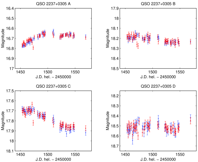
Figure 1: QSO 2237+0305 light curves in the $V$ (blue dots) and $R$ (red dots) bands obtained with PSF photometry. We have added the mean difference $V-R$ to the $R$ light curves for comparison.

Figure 2: QSO 2237+0305 light curves in the $V$ (blue dots) and $R$ (red dots) bands obtained with ISIS photometry. We have added the mean difference $V-R$ to the $R$ light curves for comparison.

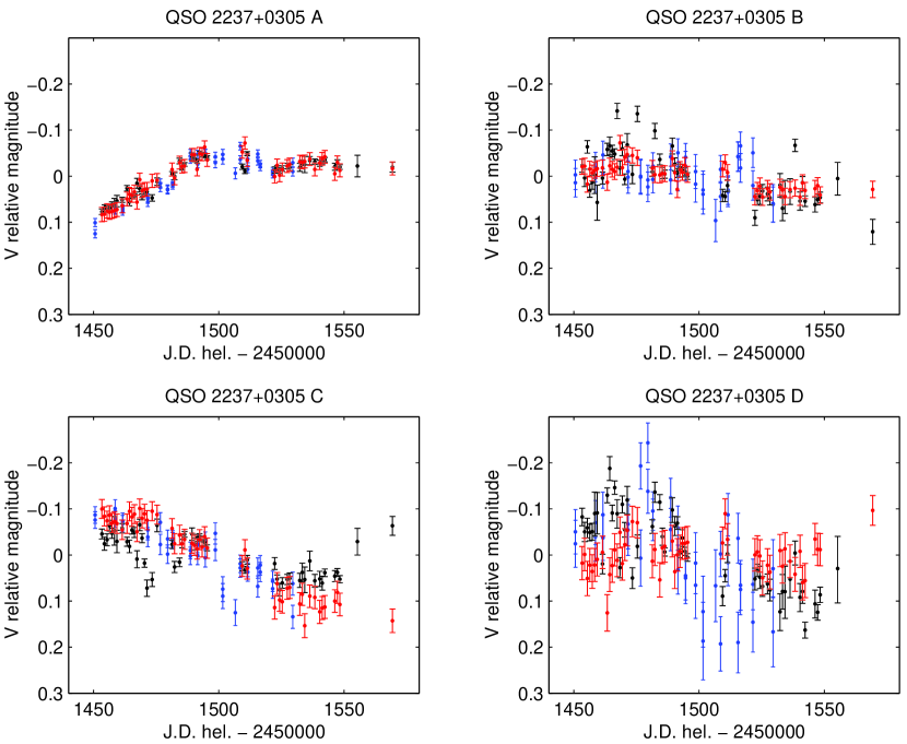
Figure 3: Comparison between GLITP/PSF (red), GLITP/ISIS (black) and OGLE (blue) QSO 2237+0305 light curves in the $V$ band. We have subtracted the mean magnitude of each component.

Table 1: Positions relative to the A component obtained by CASTLES in the $H$ band and by GLITP/PSF in the $R$ and $V$ bands

Comp.	$H$ CASTLES		$R$ GLITP/PSF		$V$ GLITP/PSF
	$\Delta$R.A. (″)	$\Delta$Dec. (″)	$\Delta$R.A. (″)	$\Delta$Dec. (″)	$\Delta$R.A. (″)	$\Delta$Dec. (″)
B	–0.673$\pm$0.003	1.697$\pm$0.003	–0.671$\pm$0.011	1.702$\pm$0.004	–0.666$\pm$0.002	1.705$\pm$0.003
C	0.635$\pm$0.003	1.209$\pm$0.003	0.638$\pm$0.008	1.204$\pm$0.006	0.640$\pm$0.001	1.205$\pm$0.003
D	–0.866$\pm$0.003	0.528$\pm$0.003	–0.868$\pm$0.007	0.531$\pm$0.005	–0.865$\pm$0.009	0.538$\pm$0.005
G	–0.075$\pm$0.003	0.939$\pm$0.003	–0.075$\pm$0.010	0.942$\pm$0.010	–0.072$\pm$0.010	0.937$\pm$0.009

Table 2: Galaxy parameters obtained by CASTLES in the $H$ band and by GLITP/PSF in the $R$ and $V$ bands

Images	$R_{\rm eff}$ (″)	$\epsilon$	P.A. (∘)
$H$ CASTLES	4.7$\pm$0.9	0.33$\pm$0.01	66$\pm$1
$R$ GLITP/PSF	4.94$\pm$0.25	0.38$\pm$0.02	62$\pm$1
$V$ GLITP/PSF	5.31$\pm$0.30	0.38$\pm$0.01	63$\pm$1

References

- Alard (2000) Alard, C. 2000, A&AS, 144, 363
- Corrigan et al. (1991) Corrigan, R. T., et al. 1991, AJ, 102, 34
- Huchra et al. (1985) Huchra, J., Gorenstein, M., Kent, S., Shapiro, I., Smith, G., Horine, E., & Perley, R. 1985, AJ, 90, 691
- Irwin et al. (1989) Irwin, M. J., Webster, R. L., Hewett, P. C., Corrigan, R. T., & Jedrzejewski, R. I. 1989, AJ, 98, 1989
- Lehár et al. (2000) Lehár, J., et al. 2000, ApJ, 536, 584
- McLeod et al. (1998) McLeod, B. A., Bernstein, G. M., Rieke, M. J., & Weedman, D. W. 1998, AJ, 115, 1377
- Østensen et al. (1996) Østensen, R., et al. 1996, A&A, 309, 59
- Remy (1996) Remy, M. 1996, PhD thesis, Université de Liège
- Schmidt, Webster, & Lewis (1998) Schmidt, R., Webster, R. L., & Lewis, G. F. 1998, MNRAS, 295, 488
- Woźniak et al. (2000a) Woźniak, P. R., Alard, C., Udalski, A., Szymański, M., Kubiak, M., Pietrzyński, G., & Zebruń, K. 2000a, ApJ, 529, 88
- Woźniak et al. (2000b) Woźniak, P. R., Udalski, A., Szymański, M., Kubiak, M., Pietrzyński, G. Soszyński, I., & Żebruń, K. 2000b, ApJ, 540, L65
- Yee (1988) Yee, H. K. C. 1988, AJ, 95, 1331